Dependence of the optical brightness on the gamma and X-ray properties of GRBs

Abstract

The Swift satellite made a real break through with measuring simultaneously the gamma X-ray and optical data of GRBs, effectively. Although, the satellite measures the gamma, X-ray and optical properties almost in the same time a significant fractions of GRBs remain undetected in the optical domain. In a large number of cases only an upper bound is obtained. Survival analysis is a tool for studying samples where a part of the cases has only an upper (lower) limit. The obtained survival function may depend on some other variables. The Cox regression is a way to study these dependencies. We studied the dependence of the optical brightness (obtained by the UVOT) on the gamma and X-ray properties, measured by the BAT and XRT on board of the Swift satellite. We showed that the gamma peak flux has the greatest impact on the afterglow’s optical brightness while the gamma photon index and the X-ray flux do not. This effect probably originates in the energetics of the jet launched from the central engine of the GRB which triggers the afterglow.

I INTRODUCTION

A significant achievement of the Swift satellite is the simultaneous detection of the physical properties of the gamma ray bursts in the gamma, X-ray and optical domain, measured by the BAT, XRT and UVOT instruments on board of the satellite.

Following the alert given by BAT the satellite starts to slew and after reaching the position of the burst the XRT and UVOT make measurements in the X-ray and optical domain, respectively.

Although, a significant fraction of the bursts is detected by the XRT as well, it is not the case with the UVOT where at a remarkable fraction of the events only an upper limit of the optical brightness is obtained.

From theoretical point of view the measured optical and gamma properties may be given by completely different phenomena, their observational relationship, if there is any, would be an important constraint for the possible models. To study this relationship it would be a serious bias if we take into account only those cases where all properties, i.e. gamma, X-ray and optical, are measured.

Survival analysis is a way to make use the information which is inherent in the value of the upper bound of the optical brightness. Cox regression is a tool for studying the dependence of the survival function (a result of the analysis) on some background variables, the covariates (gamma and X-ray properties in our case).

In the following we use Cox regression to study the dependence of the distribution of the UVOT detected optical brightness on measured gamma and X-ray properties.

II MATHEMATICAL SUMMARY

Let we have a $t$ stochastic variable with $f(t)$ probability density. The $S(t)$ survival function is defined by

$$\int\limits^{t}_{-\infty}f(t^{\prime})dt^{\prime}=F(t)=1-S(t)$$ (1)

where $F(t)$ means the probability distribution function. Actually, the $S(t)$ survival function is its complement $(F(t)+S(t)=1)$. Kaplan and Meyer (1958) showed that $S(t)$ can be estimated bias free even in the case when some of the values in the $t_{1},t_{2},\ldots,t_{n}$ observed sample are only lower bounds (censored). The ratio of $f(t)$ to $S(t)$ is called the hazard function:

$$h(t)=\frac{f(t)}{S(t)}=-\frac{S^{\prime}(t)}{S(t)}=-\frac{d}{dt}log[S(t)]$$ (2)

The $h(t)$ hazard function characterizes the risk that in the $[t,\infty]$ range $(S(t)$ gives its probability) an event will happen in the $[t,t+dt]$ interval (its unconditional probability is $f(t)dt)$. The hazard function may depend on background variables (the covariates). The Cox model (Cox (1972)) assumes that this dependency can be written in the form of

$$log[h(t)]=\alpha(t)+B_{1}x_{1}+B_{2}x_{2}+\ldots+B_{m}x_{m}$$ (3)

where $x_{1},x_{2},\ldots,x_{m}$ are the covariates while the $\alpha(t)$ arbitrary function and the $B_{1},B_{2},\ldots,B_{m}$ constants have to be determined during the procedure of the Cox regression. If all these constants are equal to zero the $\alpha(t)$ function is identical with the logarithmic hazard function. The value of the constants characterize the strengths of the influence of covariates on the hazard and, consequently on the survival function.

III DESCRIPTION OF THE DATA

We used for the present analysis the data available in the Swift table recorded until the date of 03/03/2012, in particular, the V magnitude as a dependent variable, Duration, Fluence, Peak flux, Photon index and early X-ray flux, as covariates in the analysis. Except of the Photon index we used logarithmic values in order to suppress the impact of the outliers on the regression.

Since the optical brightness of the GRB afterglow is seriously dimmed by the foreground Galactic extinction we excluded the cases with the latitude of $|b|<15^{o}(|\sin b|<0.26)$.

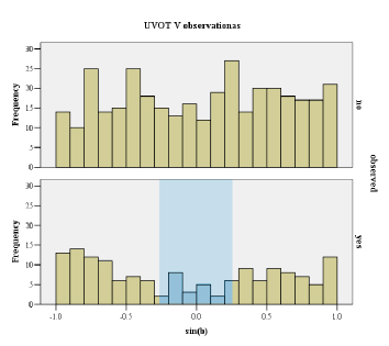
Figure 1: Distribution of the GRB positions according to the Galactic latitude. Note the depression in the distribution close to low latitudes due to the foreground extinction of the Galactic dust. Shadowed region marks the excluded area.

In the case if no afterglow was observed a lower bound in the stellar magnitude (upper bound for the observed brightness) was obtained. One can infer from Fig. 1 that at low latitudes the depression is not present in the distribution of the cases where only a lower V magnitue bound was determined.

IV COX REGRESSION

Before we make the Cox regression running we have computed the bivariate correlations between the variables included in the analysis. In this procedure we have taken into account only those cases where both variable used for computing the correlation had measured values. To overcome the problem with the outliers we computed the Spearman’s rank correlation which is not sensitive to these.

Table 1: Spearmann’s correlations (numbers in bold face mark significant correlations)

		T90	Flu	Peak	Pind	Xflu	V
T90	corr.	1.000	.646	-.066	.155	.408	-.024
	sign.	-	$<$.001	.149	.001	$<$.001	.646
Flu	corr.	.646	1.000	.539	-.148	.471	-.204
	sign.	$<$.001	-	$<$.001	.001	$<$.001	.000
Peak	corr.	-.066	.539	1.000	-.282	.141	-.289
	sign.	.149	$<$.001	-	$<$.001	.018	$<$.001
Pind	corr.	.155	-.148	-.282	1.000	.049	.004
	sign.	.001	.001	$<$.001	-	.406	.944
Xflu	corr.	.408	.471	.141	.049	1.000	-.109
	sign.	$<$.001	$<$.001	.018	.406	-	.080
V	corr.	-.024	-.204	-.289	.004	-.109	1.000
	sign.	.646	$<$.001	$<$.001	.944	.080	-

In Table 1 we used all cases having measured values in both variables used in the analysis, pairwise. We marked with bold face where the correlation coefficients differ significantly from zero. As we are approaching the detection limit of UVOT, however, only a lower magnitude limit is obtained in an increasing number of cases (see Fig. 2). Of course, cases having only an lower limit in V have to be excluded from computing the correlation of this variable with the other ones.

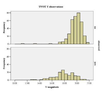
Figure 2: Distribution of the afterglows’ brightness in visual magnitude. Note the increasing fraction of censored data as we are approaching the detection limit.

Table 2: Estimated $B$ coefficients in Eq. (3) (number in bold face means that the corresponding $B$ differs from zero significantly.)

	B	Wald	df	sign.
logT90	.732	6.346	1	.012
logFlu	-.809	4.099	1	.043
logPeak	1.886	25.438	1	.000
Pind	.058	.055	1	.815
logXflu	-.003	.001	1	.973

Results of the Cox regression are summarized in Table 2. Seemingly, the duration, gamma fluence and peak flux has a significant impact on the distribution of the optical brightness, while the gamma photon index and the early X-ray flux do not.

V CONCLUSIONS

We performed Cox regression in order to look for the impact of the gamma and X-ray properties of the GRBs on the afterglows’ optical brightness. This approach is necessary since in a significant fraction of cases only an upper bound of the optical brightness (lower bound in the V magnitude) can be determined.

The analysis demonstrated that among the $B$ coefficients in Eq. (3) belonging to the duration, fluence and peak flux differ significantly from zero. Nevertheless, it is not the case with the gamma photon index and the early X-ray flux.

The reason for the impact of some gamma properties on the optical brightness is probably lying in the energetics of the jet launched from the central engine of the GRB which triggers the afterglow in the surrounding interstellar matter.