A Cyclic Douglas–Rachford Iteration Scheme

Abstract

In this paper we present two Douglas–Rachford inspired iteration schemes which can be applied directly to $N$-set convex feasibility problems in Hilbert space. Our main results are weak convergence of the methods to a point whose nearest point projections onto each of the $N$ sets coincide. For affine subspaces, convergence is in norm. Initial results from numerical experiments, comparing our methods to the classical (product-space) Douglas–Rachford scheme, are promising.

1 Introduction

Given $N$ closed and convex sets with nonempty intersection, the $N$-set convex feasibility problem asks for a point contained in the intersection of the $N$ sets. Many optimization and reconstruction problems can be cast in this framework, either directly or as a suitable relaxation if a desired bound on the quality of the solution is known a priori.

A common approach to solving $N$-set convex feasibility problems is the use of projection algorithms. These iterative methods assume that the projections onto each of the individual sets are relatively simple to compute. Some well known projection methods include von Neumann’s alternating projection method [38, 26, 17, 3, 6, 28, 29, 34], the Douglas–Rachford method [20, 31, 10] and Dykstra’s method [22, 16, 4]. Of course, there are many variants. For a review, we refer the reader to any of [2, 5, 19, 37, 24, 13].

On certain classes of problems, various projection methods coincide with each other, and with other known techniques. For example, if the sets are closed affine subspaces, alternating projections $=$ Dykstra’s method [16]. If the sets are hyperplanes, alternating projections $=$ Dykstra’s method $=$ Kaczmarz’s method [19]. If the sets are half-spaces, alternating projections $=$ the method Agmon, Motzkin and Schoenberg (MAMS), and Dykstra’s method $=$ Hildreth’s method [24, Chapter 4]. Applied to the phase retrieval problem, alternating projections $=$ error reduction, Dykstra’s method $=$ Fienup’s BIO, and Douglas–Rachford $=$ Fienup’s HIO [8].

Continued interest in the Douglas–Rachford iteration is in part due to its excellent—if still largely mysterious—performance on various problems involving one or more non-convex sets. For example, in phase retrieval problems arising in the context of image reconstruction [8, 9]. The method has also been successfully applied to NP-complete combinatorial problems including Boolean satisfiability [23, 25] and Sudoku [23, 36]. In contrast, von Neumann’s alternating projection method applied to such problems often fails to converge satisfactorily. For progress on the behaviour of non-convex alternating projections, we refer the reader to [30, 11, 27, 21].

Recently, Borwein and Sims [14] provided limited theoretical justification for non-convex Douglas–Rachford iterations, proving local convergence for a prototypical Euclidean case involving a sphere and an affine subspace. For the two-dimensional case of a circle and a line, Borwein and Aragón [1] were able to give an explicit region of convergence. Even more recently, a local version of firm nonexpansivity has been utilized by Hesse and Luke [27] to obtain local convergence of the Douglas–Rachford method in limited non-convex settings. Their results do not directly overlap with the work of Aragón, Borwein and Sims (for details see [27, Example 43]).

Most projection algorithms can be extended in various natural ways to the $N$-set convex feasibility problem without significant modification. An exception is the Douglas–Rachford method, for which only the theory of $2$-set feasibility problems has so far been successfully investigated. For applications involving $N>2$ sets, an equivalent $2$-set feasibility problem can, however, be posed in a product space. We shall revisit this later in our paper.

The aim of this paper is to introduce and study the cyclic Douglas–Rachford and averaged Douglas–Rachford iteration schemes. Both can be applied directly to the $N$-set convex feasibility problem without recourse to a product space formulation.

The paper is organized as follows: In Section 2, we give definitions and preliminaries. In Section 3, we introduce the cyclic and averaged Douglas–Rachford iteration schemes, proving in each case weak convergence to a point whose projections onto each of the constraint sets coincide. In Section 4, we consider the important special case when the constraint sets are affine. In Section 5, the new cyclic Douglas–Rachford scheme is compared, numerically, to the classical (product-space) Douglas–Rachford scheme on feasibility problems having ball or sphere constraints. Initial numerical results for the cyclic Douglas–Rachford scheme are quite positive.

2 Preliminaries

Throughout this paper,

$$\mathcal{H}\text{ is a real Hilbert space with inner product }\langle\cdot,\cdot\rangle$$

and induced norm $\|\cdot\|$. We use $\stackrel{{\scriptstyle w.}}{{\rightharpoonup}}$ to denote weak convergence.

We consider the $N$-set convex feasibility problem:

$$\text{Find~{}}~{}x\in\bigcap_{i=1}^{N}C_{i}\neq\emptyset~{}\text{ where }C_{i}\subseteq\mathcal{H}\text{ are closed and convex}.$$ (1)

Given a set $S\subseteq\mathcal{H}$ and point $x\in\mathcal{H}$, the best approximation to $x$ from $S$ is a point $p\in S$ such that

$$\|p-x\|=d(x,S):=\inf_{s\in S}\|x-s\|.$$

If for every $x\in\mathcal{H}$ there exists such a $p$, then $S$ is said to be proximal. Additionally, if $p$ is always unique then $S$ is said to be Chebyshev. In the latter case, the projection onto $S$ is the operator $P_{S}:\mathcal{H}\to S$ which maps $x$ to its unique nearest point in $S$ and we write $P_{S}(x)=p$. The reflection about $S$ is the operator $R_{S}:\mathcal{H}\to\mathcal{H}$ defined by $R_{S}:=2P_{S}-I$ where $I$ denotes the identity operator which maps any $x\in\mathcal{H}$ to itself.

Fact 2.1.

Let $C\subseteq\mathcal{H}$ be non-empty closed and convex. Then:

1. $C$ is Chebyshev.

2. (Characterization of projections)

   $$P_{C}(x)=p\iff\langle x-p,c-p\rangle\leq 0\text{ for all }c\in C.$$

3. (Characterization of reflections)

   $$R_{C}(x)=r\iff\langle x-r,c-r\rangle\leq\frac{1}{2}\|x-r\|^{2}\text{ for all }c\in C.$$

4. (Translation formula) For $y\in\mathcal{H}$, $P_{y+C}(x)=y+P_{C}(x-y)$.

5. (Dilation formula) For $0\neq\lambda\in\mathbb{R}$, $P_{\lambda C}(x)=\lambda P_{C}(x/\lambda)$.

6. If $C$ is a subspace then $P_{C}$ is linear.

7. If $C$ is an affine subspace then $P_{C}$ is affine.

Proof.

See, for example, [7, Theorem 3.14, Proposition 3.17, Corollary 3.20], [24, Theorem 2.8, Exercise 5.2(i), Theorem 3.1, Exercise 5.10] or [37, Theorem 2.1.3, Theorem 2.1.6]. Note, the equivalence of (ii) and (iii) by substituting $r=2p-x$. ∎

Given $A,B\subseteq\mathcal{H}$ we define the $2$-set Douglas–Rachford operator $T_{A,B}:\mathcal{H}\to\mathcal{H}$ by

$$T_{A,B}:=\frac{I+R_{B}R_{A}}{2}.$$ (2)

Note that $T_{A,B}$ and $T_{B,A}$ are typically distinct, while for an affine set $A$ we have $T_{A,A}=I$.

The basic Douglas–Rachford algorithm originates in [20] and convergence was proven as part of [31].

Theorem 2.1 (Douglas–Rachford [20], Lions–Mercier [31]).

Let $A,B\subseteq\mathcal{H}$ be closed and convex with nonempty intersection. For any $x_{0}\in\mathcal{H}$, the sequence $T_{A,B}^{n}x_{0}$ converges weakly to a point $x$ such that ${P_{A}x\in A\cap B}$.

Theorem 2.1 gives an iterative algorithm for solving $2$-set convex feasibility problems. For applications involving $N>2$ sets, an equivalent $2$-set formulation is posed in the product space $\mathcal{H}^{N}$. This is discussed in detail in Remark 3.4.

Let $T:\mathcal{H}\to\mathcal{H}$. We recall that $T$ is asymptotically regular if $T^{n}x-T^{n+1}x\to 0$, in norm, for all $x\in\mathcal{H}$. We denote the set of fixed points of $T$ by $\operatorname{Fix}T=\{x:Tx=x\}$. Let $D\subseteq\mathcal{H}$ and $T:D\to\mathcal{H}$. We say $T$ is nonexpansive if

$$\|Tx-Ty\|\leq\|x-y\|\text{ for all }x,y\in D$$

(i.e. $1$-Lipschitz). We say $T$ is firmly nonexpansive if

$$\|Tx-Ty\|^{2}+\|(I-T)x-(I-T)y\|^{2}\leq\|x-y\|^{2}\text{ for all }x,y\in D.$$

It immediately follows that every firmly nonexpansive mapping is nonexpansive.

Fact 2.2.

Let $A,B\subseteq\mathcal{H}$ be closed and convex. Then $P_{A}$ is firmly nonexpansive, $R_{A}$ is nonexpansive and $T_{A,B}$ is firmly nonexpansive.

Proof.

See, for example, [7, Proposition 4.8, Corollary 4.10, Remark 4.24], or [37, Theorem 2.2.4, Corollary 4.3.6]. ∎

The class of nonexpansive mappings is closed under convex combinations, compositions, etc. The class of firmly nonexpansive mappings is, however, not so well behaved. For example, even the composition of two projections onto subspaces need not be firmly nonexpansive (see [6, Example 4.2.5]).

A sufficient condition for firmly nonexpansive operators to be asymptotically regular is the following.

Lemma 2.1.

Let $T:\mathcal{H}\to\mathcal{H}$ be firmly nonexpansive with $\operatorname{Fix}T\neq\emptyset$. Then $T$ is asymptotically regular.

Proof.

See, for example, [35, Corollary 1] or [37, Lemma 4.3.5]. ∎

The composition of firmly nonexpansive operators is always nonexpansive. However, nonexpansive operators need not be asymptotically regular. For example, reflection with respect to a singleton, clearly is not; nor are most rotations. The following is a sufficient condition for asymptotic regularity.

Lemma 2.2.

Let $T_{i}:\mathcal{H}\to\mathcal{H}$ be firmly nonexpansive, for each $i$, and define $T:=T_{r}\dots T_{2}\,T_{1}$. If $\operatorname{Fix}T\neq\emptyset$ then $T$ is asymptotically regular.

Proof.

See, for example, [7, Theorem 5.22]. ∎

Remark 2.1.

Recently Bauschke, Martín-Márquez, Moffat and Wang [12, Theorem 4.6] showed that any composition of firmly nonexpansive, asymptotically regular operators is also asymptotically regular, even when $\operatorname{Fix}T=\emptyset$. $\Diamond$

The follow lemma characterizes fixed points of certain compositions of firmly nonexpansive operators.

Lemma 2.3.

Let $T_{i}:\mathcal{H}\to\mathcal{H}$ be firmly nonexpansive, for each $i$, and define $T:=T_{r}\dots T_{2}\,T_{1}$. If $\bigcap_{i=1}^{r}\operatorname{Fix}T_{i}\neq\emptyset$ then $\operatorname{Fix}T=\bigcap_{i=1}^{r}\operatorname{Fix}T_{i}$.

Proof.

See, for example, [7, Corollary 4.37]. ∎

There are many way to prove Theorem 2.1. One is to use the following well-known theorem of Opial [33].

Theorem 2.2 (Opial).

Let $T:\mathcal{H}\to\mathcal{H}$ be nonexpansive, asymptotically regular, and $\operatorname{Fix}T\neq\emptyset$. Then for any $x_{0}\in\mathcal{H}$, $T^{n}x_{0}$ converges weakly to an element of $\operatorname{Fix}T$.

Proof.

See also, for example, [33] or [7, Theorem 5.13]. ∎

In addition, when $T$ is linear, the limit can be identified and convergence is in norm.

Theorem 2.3.

Let $T:\mathcal{H}\to\mathcal{H}$ be linear, nonexpansive and asymptotically regular. Then for any $x_{0}\in\mathcal{H}$, in norm,

$$\lim_{n\to\infty}T^{n}x_{0}=P_{\operatorname{Fix}T}x_{0}.$$

Proof.

See, for example, [7, Proposition 5.27]. ∎

Remark 2.2.

A version of Theorem 2.3 was used by Halperin [26] to show that von Neumann’s alternating projection, applied to finitely many closed subspaces, converges in norm to the projection on the intersection of the subspaces. $\Diamond$

Summarizing, we have the following.

Corollary 2.1.

Let $T_{i}:\mathcal{H}\to\mathcal{H}$ be firmly nonexpansive, for each $i$, with $\bigcap_{i=1}^{r}\operatorname{Fix}T_{i}\neq\emptyset$ and define $T:=T_{r}\dots T_{2}T_{1}$. Then for any $x_{0}\in\mathcal{H}$, $T^{n}x_{0}$ converges weakly to an element of $\operatorname{Fix}T=\bigcap_{i=1}^{N}\operatorname{Fix}T_{i}$. Moreover, if $T$ is linear, then $T^{n}x_{0}$ converges, in norm, to $P_{\operatorname{Fix}T}x_{0}$.

Proof.

Since $T$ is the composition of nonexpansive operators, $T$ is nonexpansive. By Lemma 2.3, $\operatorname{Fix}T\neq\emptyset$. By Lemma 2.2, $T$ is asymptotically regular. The result now follows by Theorem 2.2 and Theorem 2.3. ∎

We note that the verification of many results in this section can be significantly simplified for the special cases we require.

3 Cyclic Douglas–Rachford Iterations

We are now ready to introduce our first new projection algorithm, the cyclic Douglas–Rachford iteration scheme. Let $C_{1},C_{2},\dots,C_{N}\subseteq\mathcal{H}$ and define $T_{[C_{1}\,C_{2}\,\dots\,C_{N}]}:\mathcal{H}\to\mathcal{H}$ by

$$T_{[C_{1}\,C_{2}\,\dots\,C_{N}]} :=T_{C_{N},C_{1}}T_{C_{N-1},C_{N}}\dots T_{C_{2},C_{3}}T_{C_{1},C_{2}}$$

$$=\left(\frac{I+R_{C_{1}}R_{C_{N}}}{2}\right)\left(\frac{I+R_{C_{N}}R_{C_{N-1}}}{2}\right)\dots\left(\frac{I+R_{C_{3}}R_{C_{2}}}{2}\right)\left(\frac{I+R_{C_{2}}R_{C_{1}}}{2}\right).$$

Given $x_{0}\in\mathcal{H}$, the cyclic Douglas–Rachford method iterates by repeatedly setting

$${x_{n+1}=T_{[C_{1}\,C_{2}\,\dots\,C_{N}]}x_{n}}.$$

Remark 3.1.

In the two set case, the cyclic Douglas–Rachford operator becomes

$$T_{[C_{1}\,C_{2}]}=T_{C_{2},C_{1}}T_{C_{1},C_{2}}=\left(\frac{I+R_{C_{1}}R_{C_{2}}}{2}\right)\left(\frac{I+R_{C_{2}}R_{C_{1}}}{2}\right).$$

That is, it does not coincide with the classic Douglas–Rachford scheme.$\Diamond$

Where there is no ambiguity, we take indices modulo $N$, and abbreviate $T_{C_{i},C_{j}}$ by $T_{i,j}$, and $T_{[C_{1}\,C_{2}\,\dots\,C_{N}]}$ by $T_{[1\,2\,\dots\,N]}$. In particular, $T_{0,1}:=T_{N,1},\,T_{N,N+1}:=T_{N,1},\,C_{0}:=C_{N}$ and $C_{N+1}:=C_{1}$.

Recall the following characterization of fixed points of the Douglas–Rachford operator.

Lemma 3.1.

Let $A,B\subseteq\mathcal{H}$ be closed and convex with nonempty intersection. Then

$$P_{A}\operatorname{Fix}T_{A,B}=A\cap B.$$

Proof.

$P_{A}\operatorname{Fix}T_{A,B}\subseteq A\cap B$ since

$$x\in\operatorname{Fix}T_{A,B}\iff\frac{x+R_{B}R_{A}x}{2}=x\iff P_{A}x=P_{B}R_{A}x\in A\cap B.$$

It is straightforward to check the reverse inclusion. ∎

We are now ready to present our main result regarding convergence of the cyclic Douglas–Rachford scheme.

Theorem 3.1 (Cyclic Douglas–Rachford).

Let $C_{1},C_{2},\dots,C_{N}\subseteq\mathcal{H}$ be closed and convex sets with a nonempty intersection. For any $x_{0}\in\mathcal{H}$, the sequence $T^{n}_{[1\,2\,\dots\,N]}x_{0}$ converges weakly to a point $x$ such that $P_{C_{i}}x=P_{C_{j}}x$, for all indices $i,j$. Moreover, $P_{C_{j}}x\in\bigcap_{i=1}^{N}C_{i}$, for each index $j$.

Proof.

By Fact 2.2, $T_{i,i+1}$ is firmly nonexpansive, for each $i$. Further,

$$\bigcap_{i=1}^{N}\operatorname{Fix}T_{i,i+1}\supseteq\bigcap_{i=1}^{N}C_{i}\neq\emptyset.$$

By Corollary 2.1, $T^{n}_{[1\,2\,\dots\,N]}x_{0}$ converges weakly to a point $x\in\operatorname{Fix}T_{[1\,2\,\dots\,N]}=\bigcap_{i=1}^{N}\operatorname{Fix}T_{i,i+1}$. By Lemma 3.1, $P_{C_{i}}x\in C_{i+1}$, for each $i$. Now we compute

$$\frac{1}{2}\sum_{i=1}^{N}\|P_{C_{i}}x-P_{C_{i-1}}x\|^{2} =\langle x,0\rangle+\frac{1}{2}\sum_{i=1}^{N}\left(\|P_{C_{i}}x\|^{2}-2\langle P_{C_{i}}x,P_{C_{i-1}}x\rangle+\|P_{C_{i-1}}x\|^{2}\right)$$

$$=\left\langle x,\sum_{i=1}^{N}(P_{C_{i-1}}x-P_{C_{i}}x)\right\rangle-\sum_{i=1}^{N}\langle P_{C_{i}}x,P_{C_{i-1}}x\rangle+\sum_{i=1}^{N}\|P_{C_{i}}x\|^{2}$$

$$=\sum_{i=1}^{N}\langle x-P_{C_{i}}x,P_{C_{i-1}}x-P_{C_{i}}x\rangle\stackrel{{\scriptstyle\text{Fact~{}\ref{fact:projections}}}}{{\leq}}0.$$

Thus, $P_{C_{i}}x=P_{C_{i-1}}x$, for each $i$; and we are done. ∎

Again by invoking Opial’s Theorem, a more general version of Theorem 3.1 can be abstracted.

Theorem 3.2.

Let $C_{1},C_{2},\dots,C_{N}\subseteq\mathcal{H}$ be closed and convex sets with nonempty intersection, let $T_{j}:\mathcal{H}\to\mathcal{H}$, for each $j$, and define $T:=T_{N}\dots T_{2}T_{1}$. Suppose the following three properties hold.

1. $T=T_{M}\dots T_{2}T_{1}$, is nonexpansive and asymptotically regular,

2. $\operatorname{Fix}T=\bigcap_{j=1}^{M}\operatorname{Fix}T_{j}\neq\emptyset$,

3. $P_{C_{j}}\operatorname{Fix}T_{j}\subseteq C_{j+1}$, for each $j$.

Then, for any $x_{0}\in\mathcal{H}$, the sequence $T^{n}x_{0}$ converges weakly to a point $x$ such that $P_{C_{i}}x=P_{C_{j}}x$ for all $i,j$. Moreover, $P_{C_{j}}x\in\bigcap_{i=1}^{N}C_{i}$, for each $j$.

Proof.

By Theorem 2.2, $T^{n}x_{0}$ converges weakly to point $x\in\operatorname{Fix}T$. The remainder of the proof is the same as Theorem 3.1. ∎

Remark 3.2.

We give a sample of examples of operators which satisfy the three conditions of Theorem 3.2.

1. $T_{[A_{1}\,A_{2}\,\dots\,A_{M}]}$ where $A_{j}\in\{C_{1},C_{2}\,\dots C_{N}\}$, and is such that each $C_{i}$ appear in the sequence $A_{1},A_{2},\dots,A_{M}$ at least once.

2. $T$ is any composition of $P_{C_{1}},P_{C_{2}},\dots,P_{C_{N}}$, such that each projection appears in said composition at least once. In particular, setting $T=P_{C_{N}}\dots P_{C_{2}}P_{C_{1}}$ we recover Bregman’s seminal result [17].

3. $T_{j}=(I+\mathbf{P}_{j})/2$ where $\mathbf{P}_{j}$ is any composition of $P_{C_{1}},P_{C_{2}},\dots,P_{C_{N}}$ such that, for each $i$, there exists a $j$ such that $\mathbf{P}_{j}=P_{C_{i}}Q_{j}$ for some composition of projections $Q_{j}$. A special case is,

   $$T=\left(\frac{I+P_{C_{1}}P_{C_{N}}}{2}\right)\dots\left(\frac{I+P_{C_{3}}P_{C_{2}}}{2}\right)\left(\frac{I+P_{C_{2}}P_{C_{1}}}{2}\right).$$

4. If $T_{1},T_{2}\dots,T_{M}$ are operators satisfying the conditions of Theorem 3.2, replacing $T_{j}$ with the relaxation $\alpha_{j}I+(1-\alpha_{j})T_{j}$ where $\alpha_{j}\in]0,1/2]$, for each $i$. Note the relaxations are firmly nonexpansive [7, Remark 4.27].

Of course, there are many other applicable variants. For instance, Krasnoselski–Mann iterations (see [7, Theorem 5.14] and [15]). $\Diamond$

We now investigate the cyclic Douglas–Rachford iteration in the special-but-common case where the initial point lies in one of the target sets; most especially the first target set.

Corollary 3.1.

Let $C_{1},C_{2},\dots,C_{N}\subseteq\mathcal{H}$ be closed and convex sets with a nonempty intersection. If $y\in C_{i}$ then $T_{i,i+1}y=P_{C_{i+1}}y$. In particular, if $x_{0}\in C_{1}$, the cyclic Douglas–Rachford trajectory coincides with that of von Neumann’s alternating projection method.

Proof.

For any $y\in\mathcal{H}$, $T_{i,i+1}y=P_{C_{i+1}}y\iff R_{C_{i+1}}y=R_{C_{i+1}}R_{C_{i}}y$. If $y\in C_{i}$ then $R_{C_{i}}y=y$. In particular, if $x_{0}\in C_{1}$ then

$$T_{[1\,2\,\dots\,N]}x_{0}=T_{N,1}\dots T_{2,3}T_{1,2}y=P_{C_{1}}P_{C_{N}}\dots P_{C_{2}}x_{0}\in C_{1},$$

and the result follows. ∎

Remark 3.3.

If $x_{0}\not\in C_{1}$, then the cyclic Douglas–Rachford trajectory need not coincide with von Neumann’s alternating projection method. We give an example involving two closed subspaces with codimension $1$ (see Figure 1). Define

$$C_{1}:=\{x\in\mathcal{H}:\langle a_{1},x\rangle=0\},\quad C_{2}:=\{x\in\mathcal{H}:\langle a_{2},x\rangle=0\},$$

where $a_{1},a_{2}\in\mathcal{H}$ such that $\langle a_{1},a_{2}\rangle\neq 0$. By scaling if necessary, we may assume that $\|a_{1}\|=\|a_{2}\|=1$. Then one has,

$$P_{C_{1}}x=x-\langle a_{1},x\rangle a_{1},\qquad P_{C_{2}}x=x-\langle a_{2},x\rangle a_{2},$$

and

$$T_{1,2}x =x+2P_{C_{2}}P_{C_{1}}x-(P_{C_{1}}x+P_{C_{2}}x)$$

$$=x-\langle a_{1},x\rangle a_{1}-\langle a_{2},x\rangle a_{2}+2\langle a_{1},a_{2}\rangle\langle a_{1},x\rangle a_{2}.$$

Similarly,

$$T_{2,1}x =x-\langle a_{1},x\rangle a_{1}-\langle a_{2},x\rangle a_{2}+2\langle a_{1},a_{2}\rangle\langle a_{2},x\rangle a_{1}.$$

By Remark 4.1,

$$2\langle a_{1},T_{[1\,2]x}\rangle =\langle a_{1},T_{1,2}x\rangle+\langle a_{1},T_{2,1}x\rangle$$

$$=\langle a_{1},x\rangle-\langle a_{1},x\rangle\|a_{1}\|^{2}-\langle a_{2},x\rangle\langle a_{1},a_{2}\rangle$$

$$\quad+\langle a_{1},a_{2}\rangle\langle a_{2},x\rangle\|a_{1}\|^{2}+\langle a_{1},a_{2}\rangle^{2}\langle a_{1},x\rangle$$

$$=\langle a_{1},a_{2}\rangle^{2}\langle a_{1},x\rangle.$$

Similarly, $2\langle a_{2},T_{[1\,2]x}\rangle=\langle a_{1},a_{2}\rangle^{2}\langle a_{2},x\rangle$.

Thus, if $\langle a_{i},x\rangle\neq 0$, for each $i$, then $\langle a_{i},T_{[1\,2]}x\rangle\neq 0$, for each $i$. In particular, if ${x_{0}\not\in C_{1}\cup C_{2}}$, then none of the cyclic Douglas–Rachford iterates lie in $C_{1}$ or $C_{2}$.

A second example, involving a ball and an affine subspace is illustrated in Figure 2. $\Diamond$

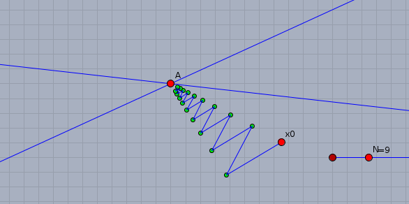
Figure 1: An interactive Cinderella applet showing a cyclic Douglas–Rachford trajectory differing from von Neumann’s alternating projection method. Each green dot represents a $2$-set Douglas–Rachford iteration.

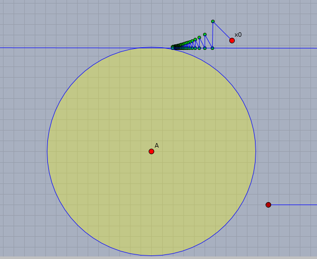
Figure 2: An interactive Cinderella applet showing a cyclic Douglas–Rachford trajectory differing from von Neumann’s alternating projection method. Each green dot represents a $2$-set Douglas–Rachford iteration.

Remark 3.4 (A product version).

We now consider the classical product formulation of (1). Define two subsets of $\mathcal{H}^{N}$:

$$C:=\prod_{i=1}^{N}C_{i},\quad D:=\{(x,x,\dots,x)\in\mathcal{H}^{N}:x\in\mathcal{H}\},$$ (3)

which are both closed and convex (in fact, $D$ is a subspace). Consider the $2$-set convex feasibility problem

$$\text{Find }\mathbf{x}\in C\cap D\subseteq\mathcal{H}^{N}.$$ (4)

Then (1) is equivalent to (4) in the sense that

$$x\in\bigcap_{i=1}^{N}C_{i}\iff(x,x,\dots,x)\in C\cap D.$$

Further the projections, and hence reflections, are easily computed since

$$P_{C}\mathbf{x}=\prod_{i=1}^{N}P_{C_{i}}\mathbf{x}_{i},\quad P_{D}\mathbf{x}=\prod_{i=1}^{N}\left(\frac{1}{N}\sum_{j=1}^{N}\mathbf{x}_{j}\right).$$

Let $\mathbf{x}_{0}\in D$ and define $\mathbf{x}_{n}:=T_{[D\,C]}\mathbf{x}_{n-1}$. Then Corollary 3.1 yields

$$T_{[D\,C]}\mathbf{x}_{n}=P_{D}P_{C}\mathbf{x}_{n}=\left(\frac{1}{N}\sum_{i=1}^{N}P_{C_{i}},\frac{1}{N}\sum_{i=1}^{N}P_{C_{i}},\dots,\frac{1}{N}\sum_{i=1}^{N}P_{C_{i}}\right).$$

That is, if—as is reasonable—we start in $D$, the cyclic Douglas–Rachford method coincides with averaged projections.

In general, the iteration is based on

$$T_{[D\,C]}\mathbf{x}=\mathbf{x}-P_{D}\mathbf{x}+2P_{D}P_{C}T_{D,C}\mathbf{x}-P_{C}T_{D,C}\mathbf{x}+P_{C}R_{D}\mathbf{x}-P_{D}P_{C}R_{D}\mathbf{x}.$$ (5)

If $\mathbf{x}=(x_{1},x_{2},\dots,x_{N})$, then the $i$th coordinate of (5) can be expressed as

$$(T_{[D\,C]}\mathbf{x})_{i} =x_{i}-\frac{1}{N}\sum_{j=1}^{N}x_{j}+\frac{2}{N}\sum_{j=1}^{N}P_{C_{j}}(T_{D,C}\mathbf{x})_{j}-P_{C_{i}}(T_{D,C}\mathbf{x})_{i}$$

$$\qquad\qquad+P_{C_{i}}\left(\frac{2}{N}\sum_{j=1}^{N}x_{j}-x_{i}\right)-\frac{1}{N}\sum_{j=1}^{N}P_{C_{j}}\left(\frac{2}{N}\sum_{k=1}^{N}x_{k}-x_{j}\right),$$

where

$$(T_{D,C}\mathbf{x})_{j} =x_{j}-\frac{1}{N}\sum_{k=1}^{N}x_{k}+P_{C_{j}}\left(\frac{2}{N}\sum_{k=1}^{N}x_{k}-x_{j}\right),$$

which is a considerably more complex formula. $\Diamond$

Let $A,B\subseteq\mathcal{H}$. Recall that points $(x,y)\in A\times B$ form a best approximation pair relative to $(A,B)$ if

$$\|x-y\|=d(A,B):=\inf\{\|a-b\|:a\in A,b\in B\}.$$

Remark 3.5.

(a) Consider $C_{1}=B_{\mathcal{H}}:=\{x\in\mathcal{H}:\|x\|\leq 1\}$ and $C_{2}=\{y\}$, for some $y\in\mathcal{H}$. Then

$$T_{[1\,2]}x=x-P_{C_{1}}x+P_{C_{1}}(y-x+P_{C_{1}}x),$$

where $P_{C_{1}}z=z$ if $z\in C_{1}$, and $z/\|z\|$ otherwise. Now,

$$x\in\operatorname{Fix}T_{[1\,2]}\iff P_{C_{1}}x=P_{C_{1}}(y-x+P_{C_{1}}x).$$ (6)

Thus,

• If $x\in C_{1}$ then $x=P_{C_{1}}y$.

• If $y-x+P_{C_{1}}x\in C_{1}$ then $x=y$.

• Else, $\|x\|>1$ and $\|y-x+P_{A}x\|>1$. By (6),

  $$x=\lambda y\text{ where }\lambda=\left(\frac{\|x\|}{\|y-x+P_{C_{1}}x\|+\|x\|-1}\right)\in]0,1[.$$

  Moreover, since $1<\|x\|=\lambda\|y\|$, we obtain $\lambda\in]1/\|y\|,1[.$

In each case, $P_{C_{1}}x=P_{C_{1}}y$ and $P_{C_{2}}x=y$. Therefore $(P_{C_{1}}x,P_{C_{2}}x)$ is a best approximation pair relative to $(C_{1},C_{2})$ (see Figure 3). In particular, if $C_{1}\cap C_{2}\neq\emptyset$, then $P_{C_{1}}y=y$ and, by Theorem 3.1, the cyclic Douglas–Rachford scheme weakly converges to $y$, the unique element of $C_{1}\cap C_{2}$.

When $C_{1}\cap C_{2}=\emptyset$, Theorem 3.1 cannot be invoked to guarantee convergence. However, the above analysis provides the information that

$$\operatorname{Fix}T_{[1\,2]}\subseteq\{\lambda P_{C_{1}}y+(1-\lambda)y:\lambda\in[0,1]\}.$$

(b) Suppose instead, $C_{1}=S_{\mathcal{H}}:=\{x\in\mathcal{H}:\|x\|=1\}$. A similar analysis can be performed. If $y\neq 0$ and $x\in\operatorname{Fix}T_{[1\,2]}$ are such that $x,y-x+P_{C_{1}}x\neq 0$, then

• If $x\in C_{1}$ then $x=P_{C_{1}}y$.

• If $y-x+P_{C_{1}}x\in C_{1}$ then $x=y$.

• Else, $x=\lambda y$ where

  $$\lambda=\left(\frac{\|x\|}{\|y-x+P_{C_{1}}x\|+\|x\|-1}\right)\geq\left(\frac{\|x\|}{\|y-x\|+\|P_{C_{1}}x\|+\|x\|-1}\right)>0.$$

Again, $(P_{C_{1}}x,P_{C_{2}}x)$ is a best approximation pair relative to $(C_{1},C_{2})$. $\Diamond$

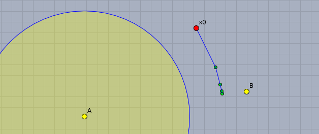
Figure 3: An interactive Cinderella applet showing the behaviour described in Remark 3.5. Each green dot represents a cyclic Douglas–Rachford iteration.

Experiments with interactive Cinderella dynamic geometry applets, suggest similar behaviour of the cyclic Douglas–Rachford method applied to many other problems for which $C_{1}\cap C_{2}=\emptyset$. For example, see Figure 4. This suggests the following conjecture.

Conjecture 3.1.

Let $C_{1},C_{2}\subseteq\mathcal{H}$ be closed and convex with $C_{1}\cap C_{2}=\emptyset$. Suppose that a best approximation pair relative to $(C_{1},C_{2})$ exists. Then the two-set cyclic Douglas–Rachford scheme converges weakly to a point $x$ such that $(P_{C_{1}}x,P_{C_{2}}x)$ is a best approximation pair relative to the sets $(C_{1},C_{2})$.

Remark 3.6.

If there exists an integer $n$ such that either $T_{[1\,2]}^{n}x_{0}\in C_{1}$ or $T_{1,2}T_{[1\,2]}^{n}x_{0}\in C_{2}$, by Corollary 3.1, the cyclic Douglas–Rachford scheme coincides with von Neumann’s alternating projection method. In this case, Conjecture 3.1 holds by [18, Theorem 2]. In this connection, we also refer the reader to [3, 4].

It is not hard to think of non-convex settings in which Conjecture 3.1 is false. For example, in $\mathbb{R}$, let $C_{1}=[0,1]$ and $C_{2}=\{0,\frac{11}{10}\}$. If $x_{0}=1$ then $T_{[1\,2]}x_{0}=x_{0}$, but

$$(P_{C_{1}}(1),P_{C_{2}}(1))=(1,\frac{11}{10}),$$

which is not a best approximation pair relative to $(C_{1},C_{2})$.$\Diamond$

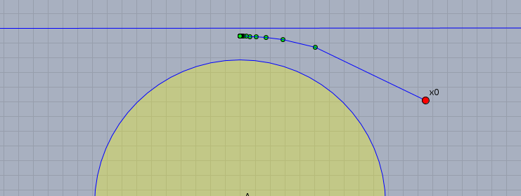
Figure 4: An interactive Cinderella applet showing the cyclic Douglas–Rachford method applied to the case of a non-intersecting ball and a line. The method appears convergent to a point whose projections onto the constraint sets form a best approximation pair. Each green dot represents a cyclic Douglas–Rachford iteration.

We now present an averaged version of our cyclic Douglas–Rachford iteration.

Theorem 3.3 (Averaged Douglas–Rachford).

Let $C_{1},C_{2},\dots,C_{N}\subseteq\mathcal{H}$ be closed and convex sets with a nonempty intersection. For any $x_{0}\in\mathcal{H}$, the sequence defined by

$$x_{n+1}:=\left(\frac{1}{N}\sum_{i=1}^{N}T_{i,i+1}\right)x_{n}$$

converges weakly to a point $x$ such that $P_{C_{i}}x=P_{C_{j}}x$ for all indices $i,j$. Moreover, ${P_{C_{j}}x\in\bigcap_{i=1}^{N}C_{i}}$, for each index $j$.

Proof.

Consider $C,D\subseteq\mathcal{H}^{N}$ as (3) and define $T:=P_{D}(\prod_{i=1}^{N}T_{i,i+1})$. By Fact 2.2, $P_{D}$ is firmly nonexpansive. By Fact 2.2, $T_{i,i+1}$ is firmly nonexpansive in $\mathcal{H}$, for each $i$, hence $\prod_{i=1}^{N}T_{i,i+1}$ is firmly nonexpansive in $\mathcal{H}^{N}$. Further, $\operatorname{Fix}(\prod_{i=1}^{N}T_{i,i+1})\cap P_{D}\supseteq C\cap D\neq\emptyset$. By Corollary 2.1, $\mathbf{x}_{n}$ converges weakly to a point $\mathbf{x}\in\operatorname{Fix}T$.

Let $\mathbf{x}_{0}=(x_{0},x_{0},\dots,x_{0})\in\mathcal{H}^{N}$. Since $T\mathbf{x}_{n}\in D$, for each $n$, we write $\mathbf{x}_{n}=(x_{n},x_{n},\dots,x_{n})$ for some $x_{n}\in\mathcal{H}$. Then

$$x_{n+1}=(T\mathbf{x}_{n+1})_{i}=\left(\frac{1}{N}\sum_{i=1}^{N}T_{i,i+1}\right)x_{n},$$

independent of $i$. Similarly, since $\mathbf{x}\in\operatorname{Fix}P_{D}=D$, we write $\mathbf{x}=(x,x,\dots,x)\in\mathcal{H}^{N}$ for some $x\in\mathcal{H}$. Since $\mathbf{x}\in\operatorname{Fix}(\prod_{i=1}^{N}T_{i,i+1})$, $x\in\operatorname{Fix}T_{i,i+1}$, for each $i$, and hence $P_{C_{i}}x\in C_{i+1}$. The same computation as in Theorem 3.1 now completes the proof. ∎

Since each $2$-set Douglas–Rachford iteration can be computed independently, the averaged iteration is easily parallelizable.

4 Affine Constraints

In this section we observe that the conclusions of Theorems 3.1 and 3.3 can be strengthened when the constraints are affine.

Lemma 4.1 (Translation formula).

Let $C_{1}^{\prime},C_{2}^{\prime},\dots,C_{N}^{\prime}\subseteq\mathcal{H}$ be closed and convex sets with a nonempty intersection. For fixed $y\in\mathcal{H}$, define $C_{i}:=y+C_{i}^{\prime}$, for each $i$. Then

$$T_{C_{i},C_{i+1}}x=y+T_{C_{i}^{\prime},C_{i+1}^{\prime}}(x-y),$$

and

$$T_{[C_{1}\,C_{2}\,\dots\,C_{N}]}x=y+T_{[C_{1}^{\prime}\,C_{2}^{\prime}\,\dots\,C_{N}^{\prime}]}(x-y).$$

Proof.

By the translation formula for projections (Fact 2.1), we have

$$R_{C_{i}}x=y+R_{C_{i}^{\prime}}(x-y),\text{ for each }i.$$

The first result follows since,

$$T_{C_{i},C_{i+1}}x =\frac{x+R_{C_{i+1}}R_{C_{i}}x}{2}=\frac{x+R_{C_{i+1}}(y+R_{C_{i}^{\prime}}(x-y))}{2}$$

$$=\frac{x+y+R_{C_{i+1}^{\prime}}R_{C_{i}^{\prime}}(x-y)}{2}=y+\frac{(x-y)+R_{C_{i+1}^{\prime}}R_{C_{i}^{\prime}}(x-y)}{2}$$

$$=y+T_{C_{i}^{\prime},C_{i+1}^{\prime}}(x-y).$$

Iterating gives,

$$T_{C_{2},C_{3}}T_{C_{1},C_{2}}=T_{C_{2},C_{3}}(y+T_{C_{1}^{\prime},C_{2}^{\prime}}(x-y))=y+T_{C_{2}^{\prime},C_{3}^{\prime}}T_{C_{1}^{\prime},C_{2}^{\prime}}(x-y),$$

from which the second result follows. ∎

Theorem 4.1 (Norm convergence).

Let $C_{1},C_{2},\cdots,C_{N}\subseteq\mathcal{H}$ be closed affine subspaces with a nonempty intersection. Then, for any $x_{0}\in\mathcal{H}$,

$$\lim_{n\to\infty}T^{n}_{[C_{1}\,C_{2}\,\dots\,C_{N}]}x_{0}=P_{\operatorname{Fix}T_{[C_{1}\,C_{2}\,\dots\,C_{N}]}}x_{0},$$

is norm convergent.

Proof.

Let $c\in\cap_{i=1}^{N}C_{i}$. Since $C_{i}$ are affine we write $C_{i}=c+C_{i}^{\prime}$, where $C_{i}^{\prime}$ is a closed subspace. Since $T_{C_{i}^{\prime},C_{i+1}^{\prime}}$ is linear, for each $i$, so is $T_{[C_{1}^{\prime}\,C_{2}^{\prime}\,\dots\,C_{N}^{\prime}]}$. By Fact 2.2, for each $i$, $T_{C_{i}^{\prime},C_{i+1}^{\prime}}$ is firmly nonexpansive. Further, $\cap_{i=1}^{N}\operatorname{Fix}T_{C_{i}^{\prime},C_{i+1}^{\prime}}\supseteq\cap_{i=1}^{N}C_{i}^{\prime}\neq\emptyset$. By Lemma 4.1 and Corollary 2.1,

$$T_{[C_{1}\,C_{2}\,\dots\,C_{N}]}^{n}x=c+T_{[C_{1}^{\prime}\,C_{2}^{\prime}\,\dots\,C_{N}^{\prime}]}^{n}(x-c)\to c+P_{\operatorname{Fix}T_{[C_{1}^{\prime}\,C_{2}^{\prime}\,\dots\,C_{N}^{\prime}]}}(x-c)=P_{\operatorname{Fix}T_{[C_{1}\,C_{2}\,\dots\,C_{N}]}}x.$$

This completes the proof. ∎

Remark 4.1.

For the case of two closed affine subspaces, the iteration becomes

$$T_{[A\,B]}=T_{B,A}T_{A,B}=\frac{I+R_{B}R_{A}+R_{A}R_{B}+R_{A}R_{B}R_{B}R_{A}}{4}=\frac{2I+R_{B}R_{A}+R_{A}R_{B}}{4}=\frac{T_{A,B}+T_{B,A}}{2}.$$

That is, the cyclic Douglas–Rachford and averaged Douglas–Rachford methods coincide.

For $N>2$ closed affine subspaces, the two methods do not always coincide. For instance, when $N=3$,

$$T_{[1\,2\,3]} =T_{3,1}T_{2,3}T_{1,2}$$

$$=I-(P_{C_{1}}+P_{C_{2}}+P_{C_{3}})+(P_{C_{1}}P_{C_{3}}+P_{C_{2}}P_{C_{1}}+P_{C_{3}}P_{C_{2}}+P_{C_{3}}P_{C_{1}}+P_{C_{1}}P_{C_{2}})$$

$$\quad-(P_{C_{3}}P_{C_{2}}P_{C_{1}}+P_{C_{1}}P_{C_{3}}P_{C_{2}}+P_{C_{1}}P_{C_{3}}P_{C_{1}}+P_{C_{1}}P_{C_{2}}P_{C_{1}})+2P_{C_{1}}P_{C_{3}}P_{C_{2}}P_{C_{1}},$$

which includes a term which is the composition of four projection operators.$\Diamond$

Theorem 4.2 (Averaged norm convergence).

Let $C_{1},C_{2},\cdots,C_{N}\subseteq\mathcal{H}$ be closed affine subspaces with a nonempty intersection. Then, in norm

$$\lim_{n\to\infty}\left(\frac{1}{M}\sum_{i=1}^{N}T_{C_{i},C_{i+1}}\right)^{n}x_{0}=P_{\operatorname{Fix}T_{[C_{1}\,C_{2}\,\dots\,C_{N}]}}x_{0}.$$

Proof.

Let $C,D\subseteq\mathcal{H}^{N}$ as in (3). Let $c\in\cap_{i=1}^{N}C_{i}$ and define $\mathbf{c}=(c,c,\dots,c)\in\mathcal{H}^{N}$. Since $C_{i}$ are affine we may write $C_{i}=c+C_{i}^{\prime}$, where $C_{i}^{\prime}$ is a closed subspace, and hence $C=\mathbf{c}+C^{\prime}$ where $C^{\prime}=\prod_{i=1}^{N}C_{i}^{\prime}$.

For convenience, let $Q$ denote $\prod_{i=1}^{N}T_{C_{i}^{\prime},C_{i+1}^{\prime}}$ and let $T=P_{D}Q$. Since $C^{\prime}$ and $D$ are subspaces, $T$ is linear. By Fact 2.2, $T_{C_{i}^{\prime},C_{i+1}^{\prime}}$ is firmly nonexpansive, hence so is $Q$. Further, $\operatorname{Fix}T\supseteq\operatorname{Fix}Q\cap\operatorname{Fix}P_{D}\supseteq\operatorname{Fix}Q\cap D\neq\emptyset$ since $\cap_{i=1}^{N}C_{i}^{\prime}\neq\emptyset$.

As a consequence of Lemma 4.1, we have the translation formula

$$T\mathbf{x}=\mathbf{c}+T(\mathbf{x}-\mathbf{c}),\text{ for any }\mathbf{x}\in\mathcal{H}^{N}.$$

As in the proof of Theorem 4.1, the translation formula, together with Corollary 2.1, shows $T^{n}\mathbf{x}_{0}\to P_{\ker T}\mathbf{x}_{0}=:\mathbf{z}$ where $\mathbf{x}_{0}=(x_{0},x_{0},\dots,x_{0})\in\mathcal{H}^{N}$. As $\mathbf{x}_{n}\in D$, we may write ${\mathbf{x}_{n}=(x_{n},x_{n},\dots,x_{n})}$ for some $x_{n}\in{\mathcal{H}}$. Similarly, we write $\mathbf{z}=(z,z,\dots,z)$. Then

$$\sqrt{N}\|x_{0}-z\| =\|\mathbf{x}_{0}-\mathbf{z}\|=d(\mathbf{x}_{0},\operatorname{Fix}T)$$

$$\leq d(\mathbf{x}_{0},(\cap_{i=1}^{N}\operatorname{Fix}T_{i,i+1})^{N})=\sqrt{N}\,d(x_{0},\cap_{i=1}^{N}\operatorname{Fix}T_{i,i+1}).$$

Hence, $z=P_{\cap_{i=1}^{N}\operatorname{Fix}T_{i,i+1}}x_{0}$. By Lemma 2.3, $\operatorname{Fix}T_{[C_{1}\,C_{2}\,\dots\,C_{N}]}=\cap_{i=1}^{N}\operatorname{Fix}T_{i,i+1}$, and the proof is complete. ∎

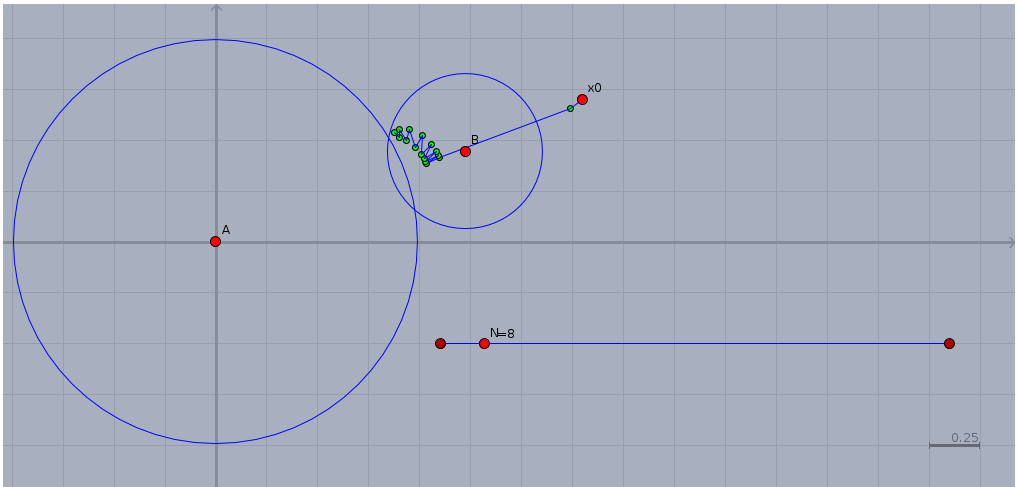
Figure 5: An interactive Cinderella applet using the cyclic Douglas–Rachford method to solve a feasibility problem with two sphere constraints. Each green dot represents a $2$-set Douglas–Rachford iteration.

5 Numerical Experiments

In this section we present the results of computational experiments comparing the cyclic Douglas–Rachford and (product-space) Douglas–Rachford schemes—as serial algorithms. These are not intended to be a complete computational study, but simply a first demonstration of viability of the method. From that vantage-point, our initial results are promising.

Two classes of feasibility problems were considered, the first convex and the second non-convex.

(P1) $$\text{Find }x\in\bigcap_{i=1}^{N}C_{i}\subseteq\mathbb{R}^{n}\text{ where }C_{i}=x_{i}+r_{i}B_{\mathcal{H}}:=\{y:\|x_{i}-y\|\leq r_{i}\},$$

(P2) $$\text{Find }x\in\bigcap_{i=1}^{N}C_{i}\subseteq\mathbb{R}^{n}\text{ where }C_{i}=x_{i}+r_{i}S_{\mathcal{H}}:=\{y:\|x_{i}-y\|=r_{i}\}.$$

Here $B_{\mathcal{H}}$ (resp. $S_{\mathcal{H}}$) denotes the closed unit ball (resp. unit sphere).

To ensure all problem instances were feasible, constraint sets were randomly generated using the following criteria.

• Ball constraints: Randomly choose $x_{i}\in[-5,5]^{n}$ and $r_{i}\in[\|x_{i}\|,\|x_{i}\|+0.1]$.

• Sphere constraints: Randomly choose $x_{i}\in[-5,5]^{n}$ and set $r_{i}=\|x_{i}\|$.

In each cases, by design, the non-empty intersection contains the origin. We consider both over- and under-constrained instances.

Note, if $C_{i}$ is a sphere constraint then $P_{C_{i}}(x_{i})=C_{i}$ (i.e., nearest points are not unique), and $P_{C_{i}}$ a set-valued mapping. In this situation, a random nearest point was chosen from $C_{i}$. In every other case, $P_{C_{i}}$ is single valued.

For the comparison, the classical Douglas–Rachford scheme was applied to the equivalent feasibility problem (4), which is formulated in the product space $(\mathbb{R}^{n})^{N}$.

Computations were performed using Python 2.6.6 on an Intel Xeon E5440 at 2.83GHz (single threaded) running 64-bit Red Hat Enterprise Linux 6.4. The following conditions were used.

• Choose a random $x_{0}\in[-10,10]^{n}$. Initialize the cyclic Douglas–Rachford scheme with $x_{0}$, and the parallel Douglas–Rachford scheme with $(x_{0},x_{0},\dots,x_{0})\in(\mathbb{R}^{n})^{N}$.

• Iterate by setting

  $$x_{n+1}=Tx_{n}\text{ where }T=T_{[1\,2\,\dots\,N]}\text{ or }T_{C,D}.$$

  An iteration limit of $1000$ was enforced.

• Stopping criterion:

  $$\|x_{n}-x_{n+1}\|<\epsilon\text{ where }\epsilon=10^{-3}\text{ or }10^{-6}.$$

• After termination, the quality of the solution was measured by

  $$\text{error}=\sum_{i=2}^{N}\|P_{C_{1}}x-P_{C_{i}}x\|^{2}.$$

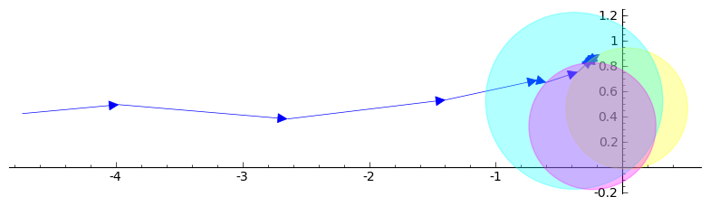
Figure 6: Cyclic Douglas–Rachford algorithm applied to a $3$-set feasibility problem in $\mathbb{R}^{2}$. The constraint sets are colored in blue, red and yellow. Each arrow represents a $2$-set Douglas–Rachford iteration.

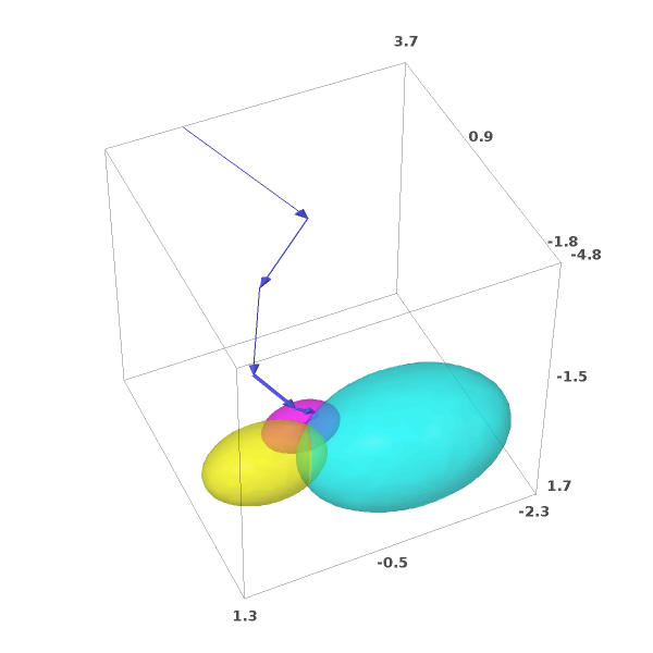
Figure 7: Cyclic Douglas–Rachford algorithm applied to a $3$-set feasibility problem in $\mathbb{R}^{3}$. The constraint sets are colored in blue, red and yellow. Each arrow represents a $2$-set Douglas–Rachford iteration.

Results are tabulated in Tables 1, 2, 3 & 4. A “$0$” error (without decimal place) represents zero within the accuracy the numpy.float64 data type. Illustrations of low dimensional examples are shown in Figures 5, 6 and 7.

We make some comments on the results.

• The cyclic Douglas–Rachford method easily solves both problems.

  Solutions for $1000$ dimensional instances, with varying numbers of constraints, could be obtained in under half-a-second, with worst case errors in the order of $10^{-13}$. Many instances of the (P1) where solved without error. Instances involving fewer constraints required a greater number of iterations before termination. This can be explained by noting that each application of $T_{[1\,2\,\dots\,N]}$ applies a $2$-set Douglas–Rachford operator $N$ times, and hence iterations for instances with a greater number of constraints are more computationally expensive.

• When the number of constraints was small, relative to the dimension of the problem, the Douglas–Rachford method was able to solve (P1) in a comparable time to the cyclic Douglas–Rachford method.

  For larger numbers of constraints the method required significantly more time. This is a consequence of working in the product space, and would be ameliorated in a parallel implementation.

• Applied to (P2), the original Douglas–Rachford method encountered difficulties.

  While it was able to solve (P2) reliably when $\epsilon=10^{-3}$, when $\epsilon=10^{-6}$ the method failed to terminate in every instance. However, in these cases the final iterate still yielded a point having a satisfactory error. The number of iterations and time required, for the Douglas–Rachford method was significantly higher compared to the cyclic Douglas–Rachford method. As with (P1), the difference was most noticeable for problems with greater numbers of constraints.

• Both methods performed better on (P1) compared to (P2).

  This might well be predicted. For in (P1), all constraint sets are convex, hence convergence is guaranteed by Theorem 3.1 and Theorem 2.1, respectively. However, in (P2), the constraints are non-convex, thus neither Theorem cannot be evoked. Our results suggest that the cyclic Douglas–Rachford as a heuristic.

• We note that there are some difficulties in using the number of iterations as a comparison between two methods.

  Each cyclic Douglas–Rachford iteration requires the computation of $2N$ reflections, and each Douglas–Rachford iteration $(N+1)$. Even taking this into account, performance of the cyclic Douglas–Rachford method was superior to the original Douglas–Rachford method on both (P1) and (P2). However, in light of the “no free lunch” theorems of Wolpert and Macready [39], we are heedful about asserting dominance of our method.

Table 1: Results for $N$ ball constraints in $\mathbb{R}^{n}$ with $\epsilon=10^{-3}$. The mean (max) from $10$ trials are reported for the cyclic Douglas–Rachford (cycDR) and Douglas–Rachford (DR) methods.

$n$	$N$	Iterations		Time (s)		Error
		cycDR	DR	cycDR	DR	cycDR	DR
100	10	4.6 (5)	22.9 (45)	0.004 (0.005)	0.022 (0.041)	0 (0)	7.91e-34 (1.65e-33)
100	20	3.4 (4)	42.4 (113)	0.006 (0.007)	0.071 (0.183)	0 (0)	1.59e-33 (6.11e-33)
100	50	2.3 (3)	75.3 (241)	0.008 (0.011)	0.288 (0.907)	2.03e-14 (2.02e-13)	6.37e-08 (6.37e-07)
100	100	2.1 (3)	97.9 (151)	0.014 (0.019)	0.717 (1.096)	0 (0)	5.51e-33 (3.85e-32)
100	200	2.0 (2)	186.2 (329)	0.025 (0.025)	2.655 (4.656)	9.68e-15 (9.68e-14)	2.17e-08 (2.17e-07)
100	500	2.0 (2)	284.2 (372)	0.059 (0.060)	9.968 (12.989)	0 (0)	2.70e-07 (9.51e-07)
100	1000	2.0 (2)	383.0 (507)	0.118 (0.119)	26.656 (35.120)	0 (0)	4.30e-07 (9.42e-07)
100	1100	2.0 (2)	380.7 (471)	0.129 (0.130)	29.160 (36.001)	0 (0)	8.35e-07 (1.79e-06)
100	1200	2.0 (2)	372.3 (537)	0.141 (0.144)	31.140 (44.886)	0 (0)	8.08e-07 (1.79e-06)
100	1500	2.0 (2)	466.0 (631)	0.178 (0.181)	49.282 (66.533)	0 (0)	5.38e-05 (5.34e-04)
100	2000	2.0 (2)	529.3 (725)	0.232 (0.234)	74.878 (102.148)	9.31e-19 (5.29e-18)	4.79e-06 (4.00e-05)
200	10	6.3 (7)	22.1 (35)	0.007 (0.008)	0.023 (0.036)	0 (0)	1.89e-33 (6.18e-33)
200	20	4.2 (5)	23.8 (56)	0.008 (0.010)	0.045 (0.103)	0 (0)	6.61e-33 (2.55e-32)
200	50	2.8 (3)	66.4 (144)	0.012 (0.013)	0.283 (0.604)	0 (0)	1.48e-32 (7.12e-32)
200	100	2.2 (3)	81.5 (132)	0.016 (0.021)	0.673 (1.083)	0 (0)	3.20e-32 (1.03e-31)
200	200	2.0 (2)	149.9 (301)	0.027 (0.028)	2.413 (4.801)	7.84e-16 (7.84e-15)	5.97e-08 (5.97e-07)
200	500	2.1 (3)	245.6 (354)	0.067 (0.095)	9.739 (14.055)	0 (0)	2.20e-07 (8.42e-07)
200	1000	2.0 (2)	323.4 (417)	0.124 (0.125)	26.429 (34.023)	0 (0)	4.10e-07 (9.43e-07)
200	1100	2.1 (3)	358.1 (434)	0.140 (0.201)	32.481 (39.289)	0 (0)	4.06e-07 (8.92e-07)
200	1200	2.0 (2)	337.0 (455)	0.145 (0.146)	33.662 (45.415)	0 (0)	8.51e-07 (1.63e-06)
200	1500	2.0 (2)	379.1 (495)	0.181 (0.183)	48.070 (62.778)	2.94e-19 (2.94e-18)	6.70e-07 (1.36e-06)
200	2000	2.0 (2)	422.6 (569)	0.239 (0.240)	74.611 (100.490)	0 (0)	7.28e-05 (7.22e-04)
500	10	9.1 (11)	17.0 (37)	0.012 (0.014)	0.023 (0.049)	0 (0)	3.19e-33 (8.23e-33)
500	20	6.1 (7)	16.9 (31)	0.014 (0.016)	0.042 (0.076)	0 (0)	2.35e-32 (6.76e-32)
500	50	3.0 (3)	66.3 (184)	0.016 (0.017)	0.373 (1.024)	0 (0)	4.55e-32 (2.23e-31)
500	100	2.6 (3)	81.5 (167)	0.023 (0.026)	0.892 (1.804)	0 (0)	2.64e-31 (1.21e-30)
500	200	2.3 (3)	142.5 (251)	0.037 (0.046)	3.068 (5.367)	0 (0)	6.58e-32 (1.90e-31)
500	500	2.0 (2)	267.3 (354)	0.071 (0.072)	15.687 (20.713)	0 (0)	2.40e-07 (1.22e-06)
500	1000	2.2 (3)	318.6 (413)	0.151 (0.204)	42.107 (54.312)	0 (0)	4.33e-07 (9.15e-07)
500	1100	2.0 (2)	338.4 (402)	0.149 (0.152)	49.911 (59.818)	0 (0)	2.45e-07 (5.58e-07)
500	1200	2.1 (3)	356.5 (478)	0.171 (0.240)	57.385 (76.217)	0 (0)	3.60e-07 (9.01e-07)
500	1500	2.0 (2)	345.7 (407)	0.203 (0.205)	70.272 (82.803)	0 (0)	6.39e-07 (9.77e-07)
500	2000	2.0 (2)	358.3 (404)	0.271 (0.273)	97.104 (110.421)	0 (0)	5.34e-07 (1.12e-06)
1000	10	15.0 (16)	12.4 (26)	0.024 (0.026)	0.023 (0.048)	2.12e-19 (2.12e-18)	1.24e-32 (3.34e-32)
1000	20	8.2 (9)	20.4 (71)	0.024 (0.027)	0.069 (0.237)	0 (0)	3.02e-32 (6.98e-32)
1000	50	4.3 (5)	38.8 (112)	0.028 (0.031)	0.311 (0.884)	2.67e-19 (2.67e-18)	1.24e-31 (5.29e-31)
1000	100	3.3 (4)	80.8 (222)	0.037 (0.042)	1.260 (3.436)	0 (0)	2.15e-31 (6.84e-31)
1000	200	2.4 (3)	138.5 (270)	0.048 (0.058)	4.730 (9.446)	0 (0)	6.50e-31 (2.52e-30)
1000	500	2.0 (2)	201.3 (313)	0.085 (0.086)	20.356 (31.166)	3.90e-20 (3.90e-19)	2.10e-30 (6.11e-30)
1000	1000	2.0 (2)	348.8 (518)	0.162 (0.164)	73.420 (108.493)	0 (0)	1.36e-06 (1.20e-05)
1000	1100	2.1 (3)	334.4 (550)	0.183 (0.260)	77.174 (126.896)	0 (0)	1.10e-07 (7.62e-07)
1000	1200	2.0 (2)	353.8 (518)	0.190 (0.193)	89.153 (128.683)	0 (0)	1.74e-07 (9.63e-07)
1000	1500	2.1 (3)	403.9 (607)	0.245 (0.346)	126.707 (189.011)	1.33e-19 (1.33e-18)	3.17e-07 (8.94e-07)
1000	2000	2.0 (2)	487.0 (593)	0.307 (0.312)	239.210 (374.390)	0 (0)	3.58e-07 (1.11e-06)

Table 2: Results for $N$ ball constraints in $\mathbb{R}^{n}$ with $\epsilon=10^{-6}$. The mean (max) from $10$ trials are reported for the cyclic Douglas–Rachford (cycDR) and Douglas–Rachford (DR) methods.

$n$	$N$	Iterations		Time (s)		Error
		cycDR	DR	cycDR	DR	cycDR	DR
100	10	4.7 (6)	22.9 (45)	0.005 (0.005)	0.023 (0.044)	0 (0)	7.91e-34 (1.65e-33)
100	20	3.6 (5)	42.4 (113)	0.006 (0.008)	0.077 (0.199)	0 (0)	1.59e-33 (6.11e-33)
100	50	2.6 (4)	77.4 (262)	0.010 (0.014)	0.320 (1.068)	0 (0)	1.24e-32 (5.96e-32)
100	100	2.1 (3)	97.9 (151)	0.015 (0.020)	0.781 (1.195)	0 (0)	5.51e-33 (3.85e-32)
100	200	2.3 (3)	187.1 (329)	0.029 (0.038)	2.909 (5.077)	0 (0)	5.89e-33 (2.30e-32)
100	500	2.3 (3)	329.6 (661)	0.071 (0.093)	12.554 (24.975)	0 (0)	1.81e-32 (6.37e-32)
100	1000	2.3 (3)	427.4 (635)	0.141 (0.184)	32.431 (47.903)	0 (0)	2.21e-32 (8.10e-32)
100	1100	2.3 (3)	467.4 (714)	0.153 (0.199)	38.936 (59.259)	0 (0)	3.92e-32 (3.17e-31)
100	1200	2.1 (3)	451.8 (698)	0.154 (0.218)	41.059 (63.259)	0 (0)	1.12e-31 (8.08e-31)
100	1500	2.1 (3)	507.2 (712)	0.193 (0.277)	58.578 (81.907)	0 (0)	2.66e-31 (8.15e-31)
100	2000	2.3 (3)	627.8 (808)	0.276 (0.361)	96.554 (124.880)	0 (0)	1.50e-31 (7.53e-31)
200	10	6.3 (7)	22.1 (35)	0.007 (0.008)	0.026 (0.040)	0 (0)	1.89e-33 (6.18e-33)
200	20	4.4 (5)	23.8 (56)	0.009 (0.010)	0.050 (0.116)	0 (0)	6.61e-33 (2.55e-32)
200	50	2.8 (3)	66.4 (144)	0.012 (0.014)	0.323 (0.691)	0 (0)	1.48e-32 (7.12e-32)
200	100	2.4 (3)	81.5 (132)	0.018 (0.022)	0.772 (1.242)	0 (0)	3.20e-32 (1.03e-31)
200	200	2.1 (3)	152.5 (301)	0.030 (0.040)	2.825 (5.547)	0 (0)	3.04e-32 (1.63e-31)
200	500	2.5 (3)	263.8 (435)	0.081 (0.098)	12.074 (19.831)	0 (0)	4.32e-32 (2.69e-31)
200	1000	2.1 (3)	427.9 (703)	0.135 (0.192)	40.025 (65.394)	0 (0)	6.64e-32 (2.66e-31)
200	1100	2.2 (3)	426.0 (545)	0.153 (0.209)	44.161 (56.724)	0 (0)	5.92e-32 (1.86e-31)
200	1200	2.2 (3)	442.9 (633)	0.166 (0.225)	50.678 (72.862)	0 (0)	5.98e-32 (2.81e-31)
200	1500	2.1 (3)	470.1 (882)	0.196 (0.279)	69.261 (128.978)	1.00e-25 (1.00e-24)	1.71e-31 (6.88e-31)
200	2000	2.0 (2)	578.4 (894)	0.248 (0.252)	117.575 (179.883)	0 (0)	4.82e-32 (1.04e-31)
500	10	9.1 (11)	17.0 (37)	0.012 (0.015)	0.028 (0.060)	0 (0)	3.19e-33 (8.23e-33)
500	20	6.1 (7)	16.9 (31)	0.015 (0.017)	0.052 (0.093)	0 (0)	2.35e-32 (6.76e-32)
500	50	3.1 (4)	66.3 (184)	0.017 (0.019)	0.467 (1.285)	0 (0)	4.55e-32 (2.23e-31)
500	100	2.6 (3)	81.5 (167)	0.024 (0.027)	1.132 (2.287)	0 (0)	2.64e-31 (1.21e-30)
500	200	2.7 (4)	142.5 (251)	0.043 (0.060)	3.979 (6.824)	0 (0)	6.58e-32 (1.90e-31)
500	500	2.1 (3)	277.5 (399)	0.078 (0.108)	20.528 (29.207)	0 (0)	4.06e-31 (2.22e-30)
500	1000	2.3 (3)	358.3 (540)	0.162 (0.210)	59.290 (88.063)	0 (0)	8.30e-32 (3.91e-31)
500	1100	2.1 (3)	372.7 (458)	0.163 (0.231)	67.065 (83.951)	0 (0)	6.41e-32 (3.21e-31)
500	1200	2.2 (3)	416.4 (604)	0.184 (0.246)	82.461 (119.456)	0 (0)	4.81e-32 (2.22e-31)
500	1500	2.1 (3)	461.7 (691)	0.220 (0.313)	114.836 (175.009)	0 (0)	2.28e-31 (1.36e-30)
500	2000	2.0 (2)	483.9 (785)	0.278 (0.283)	159.287 (259.033)	0 (0)	6.06e-31 (2.92e-30)
1000	10	15.1 (17)	12.4 (26)	0.024 (0.027)	0.030 (0.063)	0 (0)	1.24e-32 (3.34e-32)
1000	20	8.2 (9)	20.4 (71)	0.025 (0.027)	0.095 (0.330)	0 (0)	3.02e-32 (6.98e-32)
1000	50	4.5 (6)	38.8 (112)	0.029 (0.035)	0.434 (1.249)	0 (0)	1.24e-31 (5.29e-31)
1000	100	3.3 (4)	80.8 (222)	0.038 (0.043)	1.761 (4.730)	0 (0)	2.15e-31 (6.84e-31)
1000	200	2.5 (3)	138.5 (270)	0.051 (0.059)	6.224 (12.089)	0 (0)	6.50e-31 (2.52e-30)
1000	500	2.3 (3)	201.3 (313)	0.099 (0.125)	26.108 (40.534)	0 (0)	2.10e-30 (6.11e-30)
1000	1000	2.1 (3)	388.7 (905)	0.174 (0.241)	103.839 (243.085)	0 (0)	2.17e-30 (1.79e-29)
1000	1100	2.3 (3)	354.4 (660)	0.205 (0.264)	120.706 (220.612)	0 (0)	2.26e-30 (9.82e-30)
1000	1200	2.3 (3)	376.3 (620)	0.223 (0.288)	161.133 (260.857)	0 (0)	1.61e-30 (1.26e-29)
1000	1500	2.2 (3)	526.0 (1000)	0.265 (0.358)	276.095 (541.502)	2.68e-22 (2.68e-21)	1.08e-09 (5.98e-09)
1000	2000	2.1 (3)	595.0 (894)	0.332 (0.469)	427.933 (646.182)	0 (0)	4.48e-31 (1.97e-30)

Table 3: Results for $N$ sphere constraints in $\mathbb{R}^{n}$ with $\epsilon=10^{-3}$. The mean (max) from $10$ trials are reported for the cyclic Douglas–Rachford (cycDR) and Douglas–Rachford (DR) methods.

$n$	$N$	Iterations		Time (s)		Error
		cycDR	DR	cycDR	DR	cycDR	DR
100	10	16.8 (17)	219.1 (327)	0.021 (0.021)	0.272 (0.421)	4.46e-13 (7.24e-13)	8.29e-06 (1.06e-05)
100	20	9.0 (9)	247.8 (314)	0.022 (0.022)	0.669 (0.873)	5.94e-14 (1.12e-13)	1.54e-05 (1.70e-05)
100	50	5.0 (5)	375.1 (481)	0.031 (0.031)	2.559 (3.307)	6.59e-18 (1.00e-17)	2.86e-05 (3.29e-05)
100	100	3.0 (3)	471.6 (806)	0.037 (0.037)	6.185 (10.904)	1.30e-20 (2.62e-20)	4.30e-05 (4.98e-05)
100	200	2.0 (2)	747.7 (1000)	0.050 (0.050)	19.932 (26.634)	3.60e-26 (4.50e-26)	5.66e-05 (6.12e-05)
100	500	2.0 (2)	1000.0 (1000)	0.127 (0.128)	64.046 (65.562)	2.56e-26 (5.32e-26)	1.18e-04 (1.40e-04)
100	1000	2.0 (2)	1000.0 (1000)	0.253 (0.255)	130.475 (138.540)	3.87e-26 (8.28e-26)	2.43e-04 (2.70e-04)
100	1100	2.0 (2)	1000.0 (1000)	0.278 (0.281)	143.022 (149.895)	5.28e-26 (8.95e-26)	2.53e-04 (2.95e-04)
100	1200	2.0 (2)	1000.0 (1000)	0.304 (0.306)	156.653 (158.918)	7.16e-26 (1.65e-25)	3.12e-04 (3.74e-04)
100	1500	2.0 (2)	1000.0 (1000)	0.380 (0.386)	197.801 (210.661)	1.02e-25 (2.27e-25)	3.50e-04 (3.84e-04)
100	2000	2.0 (2)	1000.0 (1000)	0.504 (0.511)	261.535 (267.483)	9.91e-26 (2.42e-25)	4.82e-04 (6.04e-04)
200	10	23.0 (23)	123.1 (222)	0.030 (0.030)	0.183 (0.334)	2.50e-13 (7.46e-13)	6.33e-06 (8.72e-06)
200	20	12.8 (13)	115.2 (171)	0.033 (0.034)	0.329 (0.507)	1.48e-14 (4.39e-14)	1.05e-05 (1.46e-05)
200	50	6.0 (6)	110.6 (124)	0.038 (0.038)	0.790 (0.874)	2.56e-16 (4.47e-16)	1.42e-05 (2.09e-05)
200	100	4.0 (4)	120.1 (128)	0.051 (0.052)	1.726 (1.825)	2.49e-20 (3.71e-20)	1.70e-05 (2.21e-05)
200	200	3.0 (3)	134.9 (139)	0.077 (0.078)	3.749 (4.088)	2.88e-26 (6.69e-26)	2.31e-05 (2.98e-05)
200	500	2.0 (2)	156.4 (161)	0.130 (0.131)	11.106 (11.715)	8.53e-26 (1.71e-25)	4.37e-05 (5.16e-05)
200	1000	2.0 (2)	175.6 (182)	0.262 (0.264)	26.888 (30.935)	1.53e-25 (3.33e-25)	7.27e-05 (8.71e-05)
200	1100	2.0 (2)	179.5 (191)	0.286 (0.290)	31.161 (33.273)	1.71e-25 (2.77e-25)	7.97e-05 (9.82e-05)
200	1200	2.0 (2)	179.0 (184)	0.309 (0.316)	31.547 (35.242)	2.02e-25 (4.76e-25)	7.86e-05 (8.59e-05)
200	1500	2.0 (2)	190.0 (200)	0.394 (0.400)	43.207 (47.057)	2.29e-25 (3.91e-25)	9.97e-05 (1.15e-04)
200	2000	2.0 (2)	230.3 (295)	0.522 (0.525)	72.760 (94.718)	3.96e-25 (7.53e-25)	1.34e-04 (1.58e-04)
500	10	35.3 (36)	51.6 (67)	0.051 (0.052)	0.093 (0.121)	4.81e-14 (1.13e-13)	1.46e-06 (2.86e-06)
500	20	19.1 (20)	72.3 (85)	0.055 (0.057)	0.254 (0.300)	8.32e-15 (1.21e-14)	2.02e-06 (3.29e-06)
500	50	9.0 (9)	96.8 (107)	0.064 (0.064)	0.888 (0.991)	1.82e-16 (2.72e-16)	2.03e-06 (2.36e-06)
500	100	5.0 (5)	120.5 (127)	0.070 (0.071)	2.271 (2.475)	1.21e-17 (1.75e-17)	2.39e-06 (2.98e-06)
500	200	3.0 (3)	143.0 (148)	0.085 (0.085)	5.579 (6.072)	4.29e-20 (5.80e-20)	2.84e-06 (3.79e-06)
500	500	2.0 (2)	171.3 (176)	0.145 (0.146)	17.719 (21.106)	3.30e-25 (8.09e-25)	4.14e-06 (4.50e-06)
500	1000	2.0 (2)	195.1 (197)	0.295 (0.296)	47.771 (51.291)	8.61e-25 (1.37e-24)	6.18e-06 (6.64e-06)
500	1100	2.0 (2)	198.1 (202)	0.327 (0.329)	50.934 (54.122)	1.02e-24 (2.28e-24)	6.93e-06 (8.30e-06)
500	1200	2.0 (2)	199.8 (204)	0.359 (0.362)	56.155 (60.472)	1.01e-24 (2.17e-24)	6.69e-06 (7.56e-06)
500	1500	2.0 (2)	208.5 (213)	0.445 (0.451)	73.848 (78.355)	1.34e-24 (2.66e-24)	7.96e-06 (8.62e-06)
500	2000	2.0 (2)	217.8 (221)	0.590 (0.598)	100.538 (111.140)	1.61e-24 (3.00e-24)	1.00e-05 (1.09e-05)
1000	10	49.2 (50)	9.1 (29)	0.083 (0.085)	0.023 (0.072)	1.32e-14 (2.44e-14)	3.15e-07 (7.11e-07)
1000	20	27.0 (27)	30.0 (66)	0.092 (0.092)	0.127 (0.276)	1.96e-15 (3.11e-15)	4.88e-07 (7.90e-07)
1000	50	12.0 (12)	73.1 (86)	0.100 (0.100)	0.779 (0.946)	1.85e-16 (2.37e-16)	4.98e-07 (6.57e-07)
1000	100	7.0 (7)	103.7 (113)	0.117 (0.117)	2.248 (2.513)	4.22e-18 (5.49e-18)	5.51e-07 (7.17e-07)
1000	200	4.0 (4)	136.8 (143)	0.133 (0.134)	8.869 (10.028)	8.89e-20 (1.1e-19)	6.28e-07 (7.86e-07)
1000	500	3.0 (3)	178.9 (182)	0.258 (0.260)	31.706 (34.394)	2.17e-24 (5.88e-24)	7.86e-07 (9.48e-07)
1000	1000	2.0 (2)	211.7 (215)	0.343 (0.344)	73.182 (78.028)	2.16e-24 (3.71e-24)	1.04e-06 (1.15e-06)
1000	1100	2.0 (2)	215.3 (221)	0.379 (0.383)	84.584 (92.095)	4.01e-24 (9.45e-24)	1.07e-06 (1.21e-06)
1000	1200	2.0 (2)	218.7 (220)	0.411 (0.414)	94.408 (99.951)	3.91e-24 (8.19e-24)	1.14e-06 (1.27e-06)
1000	1500	2.0 (2)	228.6 (232)	0.518 (0.524)	124.265 (132.683)	5.73e-24 (1.58e-23)	1.29e-06 (1.48e-06)
1000	2000	2.0 (2)	242.3 (245)	0.681 (0.684)	176.575 (191.354)	6.06e-24 (1.5e-23)	1.53e-06 (1.67e-06)

Table 4: Results for $N$ sphere constraints in $\mathbb{R}^{n}$ with $\epsilon=10^{-6}$. The mean (max) from $10$ trials are reported for the cyclic Douglas–Rachford (cycDR) and Douglas–Rachford (DR) methods.

$n$	$N$	Iterations		Time (s)		Error
		cycDR	DR	cycDR	DR	cycDR	DR
100	10	27.4 (28)	1000.0 (1000)	0.035 (0.036)	1.302 (1.419)	1.21e-18 (2.25e-18)	9.10e-08 (2.16e-07)
100	20	14.1 (15)	1000.0 (1000)	0.036 (0.038)	2.463 (2.750)	1.21e-19 (2.65e-19)	1.26e-06 (1.78e-06)
100	50	7.0 (7)	1000.0 (1000)	0.044 (0.045)	6.760 (7.052)	1.02e-23 (1.81e-23)	8.51e-06 (1.07e-05)
100	100	4.0 (4)	1000.0 (1000)	0.052 (0.052)	13.823 (14.145)	2.02e-26 (3.73e-26)	2.17e-05 (3.00e-05)
100	200	3.0 (3)	1000.0 (1000)	0.078 (0.078)	25.239 (27.594)	8.97e-27 (1.69e-26)	4.39e-05 (5.93e-05)
100	500	2.0 (2)	1000.0 (1000)	0.131 (0.132)	66.159 (68.491)	2.56e-26 (5.32e-26)	1.18e-04 (1.40e-04)
100	1000	2.0 (2)	1000.0 (1000)	0.262 (0.263)	131.165 (139.166)	3.87e-26 (8.28e-26)	2.43e-04 (2.70e-04)
100	1100	2.0 (2)	1000.0 (1000)	0.290 (0.293)	149.386 (154.285)	5.28e-26 (8.95e-26)	2.53e-04 (2.95e-04)
100	1200	2.0 (2)	1000.0 (1000)	0.317 (0.322)	162.476 (171.252)	7.16e-26 (1.65e-25)	3.12e-04 (3.74e-04)
100	1500	2.0 (2)	1000.0 (1000)	0.395 (0.399)	205.210 (214.347)	1.02e-25 (2.27e-25)	3.50e-04 (3.84e-04)
100	2000	2.0 (2)	1000.0 (1000)	0.524 (0.527)	284.740 (295.621)	9.91e-26 (2.42e-25)	4.82e-04 (6.04e-04)
200	10	37.8 (39)	1000.0 (1000)	0.051 (0.053)	1.787 (1.801)	5.36e-19 (9.86e-19)	9.14e-08 (1.73e-07)
200	20	20.0 (20)	1000.0 (1000)	0.053 (0.054)	3.422 (3.452)	2.01e-20 (3.49e-20)	9.56e-07 (1.46e-06)
200	50	9.0 (9)	1000.0 (1000)	0.059 (0.060)	8.384 (8.615)	1.53e-22 (3.08e-22)	4.52e-06 (6.27e-06)
200	100	5.0 (5)	1000.0 (1000)	0.067 (0.067)	15.429 (17.471)	1.61e-24 (2.45e-24)	8.05e-06 (1.09e-05)
200	200	3.0 (3)	1000.0 (1000)	0.080 (0.080)	31.967 (33.857)	2.88e-26 (6.69e-26)	1.39e-05 (1.8e-05)
200	500	2.0 (2)	1000.0 (1000)	0.135 (0.135)	81.272 (85.423)	8.53e-26 (1.71e-25)	3.07e-05 (3.64e-05)
200	1000	2.0 (2)	1000.0 (1000)	0.272 (0.273)	166.615 (177.342)	1.53e-25 (3.33e-25)	5.49e-05 (6.55e-05)
200	1100	2.0 (2)	1000.0 (1000)	0.297 (0.299)	168.501 (184.769)	1.71e-25 (2.77e-25)	6.05e-05 (7.36e-05)
200	1200	2.0 (2)	1000.0 (1000)	0.320 (0.323)	195.997 (204.751)	2.02e-25 (4.76e-25)	6.03e-05 (6.58e-05)
200	1500	2.0 (2)	1000.0 (1000)	0.411 (0.416)	250.555 (257.482)	2.29e-25 (3.91e-25)	7.77e-05 (9.00e-05)
200	2000	2.0 (2)	1000.0 (1000)	0.540 (0.543)	333.273 (340.514)	3.96e-25 (7.53e-25)	1.06e-04 (1.29e-04)
500	10	58.0 (59)	1000.0 (1000)	0.085 (0.087)	2.135 (2.220)	1.46e-19 (3.30e-19)	7.50e-08 (1.05e-07)
500	20	30.8 (31)	1000.0 (1000)	0.091 (0.091)	3.658 (3.691)	1.04e-20 (2.56e-20)	4.45e-07 (6.81e-07)
500	50	13.1 (14)	1000.0 (1000)	0.095 (0.102)	9.321 (10.090)	8.52e-22 (1.38e-21)	1.05e-06 (1.21e-06)
500	100	7.8 (8)	1000.0 (1000)	0.114 (0.117)	18.124 (19.334)	8.23e-24 (4.40e-23)	1.65e-06 (2.04e-06)
500	200	5.0 (5)	1000.0 (1000)	0.147 (0.147)	41.555 (45.159)	1.60e-25 (2.81e-25)	2.25e-06 (2.95e-06)
500	500	3.0 (3)	1000.0 (1000)	0.224 (0.225)	118.550 (125.955)	3.31e-25 (8.15e-25)	3.60e-06 (3.91e-06)
500	1000	2.0 (2)	1000.0 (1000)	0.305 (0.306)	256.931 (276.971)	8.61e-25 (1.37e-24)	5.57e-06 (5.97e-06)
500	1100	2.0 (2)	1000.0 (1000)	0.336 (0.338)	279.305 (295.475)	1.02e-24 (2.28e-24)	6.26e-06 (7.46e-06)
500	1200	2.0 (2)	1000.0 (1000)	0.369 (0.371)	299.386 (318.799)	1.01e-24 (2.17e-24)	6.06e-06 (6.85e-06)
500	1500	2.0 (2)	1000.0 (1000)	0.459 (0.465)	379.780 (394.991)	1.34e-24 (2.66e-24)	7.28e-06 (7.89e-06)
500	2000	2.0 (2)	1000.0 (1000)	0.610 (0.618)	513.325 (526.365)	1.61e-24 (3.00e-24)	9.24e-06 (1.01e-05)
1000	10	81.1 (82)	1000.0 (1000)	0.140 (0.141)	3.181 (3.250)	4.17e-20 (8.76e-20)	3.62e-08 (9.00e-08)
1000	20	42.9 (43)	1000.0 (1000)	0.148 (0.149)	6.256 (6.973)	3.33e-21 (5.35e-21)	1.65e-07 (2.59e-07)
1000	50	18.8 (19)	1000.0 (1000)	0.161 (0.164)	15.651 (17.205)	1.26e-22 (4.37e-22)	3.17e-07 (4.18e-07)
1000	100	10.0 (10)	1000.0 (1000)	0.172 (0.172)	32.247 (36.360)	9.71e-24 (1.23e-23)	4.33e-07 (5.66e-07)
1000	200	6.0 (6)	1000.0 (1000)	0.207 (0.208)	71.902 (79.069)	6.31e-25 (1.43e-24)	5.46e-07 (6.82e-07)
1000	500	3.0 (3)	1000.0 (1000)	0.261 (0.263)	199.425 (211.841)	2.17e-24 (5.88e-24)	7.24e-07 (8.72e-07)
1000	1000	2.0 (2)	1000.0 (1000)	0.352 (0.354)	366.672 (403.696)	2.16e-24 (3.71e-24)	9.80e-07 (1.08e-06)
1000	1100	2.0 (2)	1000.0 (1000)	0.391 (0.393)	388.322 (396.817)	4.01e-24 (9.45e-24)	1.01e-06 (1.14e-06)
1000	1200	2.0 (2)	1000.0 (1000)	0.426 (0.427)	426.523 (436.721)	3.91e-24 (8.19e-24)	1.08e-06 (1.20e-06)
1000	1500	2.0 (2)	1000.0 (1000)	0.526 (0.535)	533.574 (546.055)	5.73e-24 (1.58e-23)	1.22e-06 (1.41e-06)
1000	2000	2.0 (2)	1000.0 (1000)	0.697 (0.700)	725.869 (733.381)	6.06e-24 (1.50e-23)	1.46e-06 (1.59e-06)

6 Conclusion

Two new projection algorithms, the cyclic Douglas–Rachford and averaged Douglas–Rachford iteration schemes, were introduced and studied. Applied to $N$-set convex feasibility problems in Hilbert space, both weakly converge to point whose projections onto each of the $N$-set coincide. While the cyclic Douglas–Rachford is sequential, each iteration of the averaged Douglas–Rachford can be parallelized.

Numerical experiments suggest that that the cyclic Douglas–Rachford scheme outperforms the classical Douglas–Rachford scheme, which suffers as a result of the product formulation. An advantage of our schemes is that they can be used in the original space, without recourse to this formulation. For inconsistent $2$-set problems, there is evidence to suggest that the two set cyclic Douglas–Rachford scheme yields best approximation pairs.

HTML versions of the interactive Cinderella applets are available at:

1. http://carma.newcastle.edu.au/tam/cycdr/2lines.html

2. http://carma.newcastle.edu.au/tam/cycdr/circleline.html

3. http://carma.newcastle.edu.au/tam/cycdr/2circles.html

4. http://carma.newcastle.edu.au/tam/cycdr/circlepoint.html

References

- [1] F.J. Aragón Artacho and J.M. Borwein. Global convergence of a non-convex Douglas–Rachford iteration. Journal of Global Optimization, pages 1–17, 2012.
- [2] H.H. Bauschke. Projection algorithms: results and open problems. Studies in Computational Mathematics, 8:11–22, 2001.
- [3] H.H. Bauschke and J.M. Borwein. On the convergence of von Neumann’s alternating projection algorithm for two sets. Set-Valued Analysis, 1(2):185–212, 1993.
- [4] H.H. Bauschke and J.M. Borwein. Dykstra’s alternating projection algorithm for two sets. Journal of Approximation Theory, 79(3):418–443, 1994.
- [5] H.H. Bauschke and J.M. Borwein. On projection algorithms for solving convex feasibility problems. SIAM review, pages 367–426, 1996.
- [6] H.H. Bauschke, J.M. Borwein, and A.S. Lewis. The method of cyclic projections for closed convex sets in Hilbert space. Contemporary Mathematics, 204:1–38, 1997.
- [7] H.H. Bauschke and P.L. Combettes. Convex Analysis and Monotone Operator Theory in Hilbert Spaces. Canadian Mathematical Society Societe Mathematique Du Canada. Springer New York, 2011.
- [8] H.H. Bauschke, P.L. Combettes, and D.R. Luke. Phase retrieval, error reduction algorithm, and Fienup variants: a view from convex optimization. JOSA A, 19(7):1334–1345, 2002.
- [9] H.H. Bauschke, P.L. Combettes, and D.R. Luke. Hybrid projection–reflection method for phase retrieval. JOSA A, 20(6):1025–1034, 2003.
- [10] H.H Bauschke, P.L. Combettes, and D.R. Luke. Finding best approximation pairs relative to two closed convex sets in Hilbert spaces. Journal of Approximation Theory, 127(2):178–192, 2004.
- [11] H.H Bauschke, D.R. Luke, H.M. Phan, and X. Wang. Restricted normal cones and the method of alternating projections. preprint http://arxiv.org/pdf/1205.0318v1, 2012.
- [12] H.H. Bauschke, V. Martín-Márquez, S.M. Moffat, and X. Wang. Compositions and convex combinations of asymptotically regular firmly nonexpansive mappings are also asymptotically regular. Fixed Point Theory and Appl., 2012(53):1–11, 2012.
- [13] J.M. Borwein. Maximum entropy and feasibility methods for convex and nonconvex inverse problems. Optimization, 61(1):1–33, 2012.
- [14] J.M. Borwein and B. Sims. The Douglas–Rachford algorithm in the absence of convexity. Fixed-Point Algorithms for Inverse Problems in Science and Engineering, pages 93–109, 2011.
- [15] Jonathan Borwein, Simeon Reich, and Itai Shafrir. Krasnoselski-Mann iterations in normed spaces. Canad. Math. Bull, 35(1):21–28, 1992.
- [16] J.P. Boyle and R.L. Dykstra. A method for finding projections onto the intersection of convex sets in Hilbert spaces. Lecture Notes in Statistics, 37(28-47):4, 1986.
- [17] L.M. Bregman. The method of successive projection for finding a common point of convex sets. Soviet Mathematics, 6:688–692, 1965.
- [18] W. Cheney and A.A Goldstein. Proximity maps for convex sets. Proceedings of the American Mathematical Society, 10(3):448–450, 1959.
- [19] F. Deutsch. The method of alternating orthogonal projections. Approximation Theory, Spline Functions and Applications, Kluwer Academic Publishers, Dordrecht, pages 105–121, 1992.
- [20] J. Douglas and H.H. Rachford. On the numerical solution of heat conduction problems in two and three space variables. Transactions of the American Mathematical Society, 82(2):421–439, 1956.
- [21] D. Drusvyatskiy, A.D. Ioffe, and A.S. Lewis. Alternating projections: a new approach. In preparation.
- [22] R.L. Dykstra. An algorithm for restricted least squares regression. Journal of the American Statistical Association, 78(384):837–842, 1983.
- [23] V. Elser, I. Rankenburg, and P. Thibault. Searching with iterated maps. Proceedings of the National Academy of Sciences, 104(2):418–423, 2007.
- [24] R. Escalante and M. Raydan. Alternating Projection Methods. Fundamentals of Algorithms. Society for Industrial and Applied Mathematics, 2011.
- [25] S. Gravel and V. Elser. Divide and concur: A general approach to constraint satisfaction. Physical Review E, 78(3):036706, 2008.
- [26] I. Halperin. The product of projection operators. Acta Sci. Math. (Szeged), 23:96–99, 1962.
- [27] R. Hesse and D.R. Luke. Nonconvex notions of regularity and convergence of fundamental algorithms for feasibility problems. preprint http://arxiv.org/pdf/1205.0318v1, 2012.
- [28] E. Kopecká and S. Reich. A note on the von Neumann alternating projections algorithm. J. Nonlinear Convex Anal, 5(3):379–386, 2004.
- [29] E. Kopecká and S. Reich. Another note on the von Neumann alternating projections algorithm. J. Nonlinear Convex Anal, 11:455–460, 2010.
- [30] A.S. Lewis, D.R. Luke, and J. Malick. Local linear convergence for alternating and averaged nonconvex projections. Foundations of Computational Mathematics, 9(4):485–513, 2009.
- [31] P.L. Lions and B. Mercier. Splitting algorithms for the sum of two nonlinear operators. SIAM Journal on Numerical Analysis, pages 964–979, 1979.
- [32] A. Netyanun and D.C. Solmon. Iterated products of projections in Hilbert space. The American Mathematical Monthly, 113(7):644–648, 2006.
- [33] Z. Opial. Weak convergence of the sequence of successive approximations for nonexpansive mappings. Bull. Amer. Math. Soc, 73(4):591–597, 1967.
- [34] E. Pustylnik, S. Reich, and A.J. Zaslavski. Convergence of non-periodic infinite products of orthogonal projections and nonexpansive operators in Hilbert space. Journal of Approximation Theory, 164(5):611–624, 2012.
- [35] S. Reich and I. Shafrir. The asymptotic behavior of firmly nonexpansive mappings. Proceedings of the American Mathematical Society, pages 246–250, 1987.
- [36] J. Schaad. Modeling the 8-queens problem and sudoku using an algorithm based on projections onto nonconvex sets. Master’s thesis, Univ. of British Columbia, 2010.
- [37] M.K. Tam. The Method of Alternating Projections. http://docserver.carma.newcastle.edu.au/id/eprint/1463, 2012. Honours thesis, Univ. of Newcastle.
- [38] J. von Neumann. Functional Operators Vol. II. The Geometry of Orthogonal Spaces, volume 22. Princeton University Press, 1950.
- [39] D.H. Wolpert and W.G. Macready. No free lunch theorems for optimization. IEEE Transactions on Evolutionary Computation, 1(1):67–82, 1997.