Simultaneous Spin-Charge Relaxation in Double Quantum Dots

Abstract

We investigate phonon-induced spin and charge relaxation mediated by spin-orbit and hyperfine interactions for a single electron confined within a double quantum dot. A simple toy model incorporating both direct decay to the ground state of the double dot and indirect decay via an intermediate excited state yields an electron spin relaxation rate that varies non-monotonically with the detuning between the dots. We confirm this model with experiments performed on a GaAs double dot, demonstrating that the relaxation rate exhibits the expected detuning dependence and can be electrically tuned over several orders of magnitude. Our analysis suggests that spin-orbit mediated relaxation via phonons serves as the dominant mechanism through which the double-dot electron spin-flip rate varies with detuning.

Controlling individual spins is central to spin-based quantum information processing Loss and DiVincenzo (1998); Hanson et al. (2007); Hanson and Awschalom (2008) and also enables precision metrology Taylor et al. (2008); Dolde et al. (2011). While rapid control can be achieved by coupling the spins of electrons in semiconductor quantum dots Loss and DiVincenzo (1998); Hanson et al. (2007) to electric fields via the electronic charge state Hanson and Awschalom (2008); Kato et al. (2003); Rashba and Efros (2003); Taylor et al. (2005); Tokura et al. (2006); Nowack et al. (2007); Laird et al. (2007); Pioro-Ladriere et al. (2008); Schreiber et al. (2011); Shafiei et al. (2013), spin-charge coupling also leads to relaxation of the spins through fluctuations in their electrostatic environment. Phonons serve as an inherent source of fluctuating electric fields in quantum dots Hanson et al. (2007) and give rise to both charge and spin relaxation through the electron-phonon interaction. In GaAs quantum dots, the direct coupling of spin to the strain field produced by phonons is expected to be inefficient Khaetskii and Nazarov (2000, 2001). The dominant mechanisms of phonon-induced spin relaxation are therefore indirect and involve spin-charge coupling due to primarily spin-orbit Khaetskii and Nazarov (2000, 2001); Golovach et al. (2004); Bulaev and Loss (2005); Stano and Fabian (2005, 2006); Amasha et al. (2008) and hyperfine Erlingsson et al. (2001); Erlingsson and Nazarov (2002); Merkulov et al. (2002); Johnson et al. (2005); Koppens et al. (2005); Taylor et al. (2007) interactions. Confining an electron within a double quantum dot (DQD) provides a high degree of control over the charge state van der Wiel et al. (2002); Hayashi et al. (2003); Petta et al. (2004); Gorman et al. (2005), so that relaxation rates can be varied over multiple orders of magnitude by adjusting the energy level detuning between the dots Fujisawa et al. (1998); Johnson et al. (2005); Raith et al. (2012); Wang and Wu (2006); Wang et al. (2011).

Here, we investigate the interplay of spin and charge relaxation via phonons for a single electron confined to a DQD in the presence of spin-orbit and hyperfine interactions. We present a simple model together with measurements of the electron spin relaxation rate in a GaAs DQD, both of which yield a non-monotonic dependence on the detuning between the dots (see Fig. 3). The experiments provide confirmation of the model and demonstrate the existence of spin “hot spot” features Fabian and Das Sarma (1998); Bulaev and Loss (2005); Stano and Fabian (2005, 2006); Raith et al. (2011) at nonzero values of detuning, where relaxation is enhanced by several orders of magnitude. The opposite behavior is observed at zero detuning, where the spin-flip rate exhibits a local minimum. Theoretically, spin hot spots are predicted to occur due to the complete mixing of spin and orbital states at avoided energy crossings associated with spin-orbit coupling Fabian and Das Sarma (1998); Bulaev and Loss (2005); Stano and Fabian (2005). From a practical standpoint, adjusting the detuning to these points represents a potential method for rapid all-electrical spin initialization.

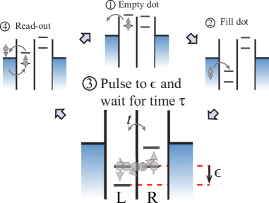
Figure 1: Electrochemical potential diagrams for a double quantum dot (DQD), illustrating the measurement cycle used to obtain the experimental spin relaxation rate (see main text). Varying the detuning $\epsilon$ between the left (L) and right (R) dots while keeping the tunnel coupling $t$ fixed (stage 3) tunes the relative energies of the charge states. Tunneling of the electron between the dots is accompanied by spin rotation.

We describe a single electron confined within a DQD (Fig. 1) using a toy model that includes only the lowest-energy orbital level of each dot. This two-level approximation van der Wiel et al. (2002) enables the charge degrees of freedom to be represented by the Pauli matrices $\sigma_{x},\sigma_{y},\sigma_{z}$ in the basis $\left\{\left|L\right\rangle,\left|R\right\rangle\right\}$, where $\left|L\right\rangle$ ($\left|R\right\rangle$) denotes an electron in the left (right) quantum dot and $\sigma_{z}\equiv\left|L\right\rangle\left\langle L\right|-\left|R\right\rangle\left\langle R\right|$. We can then express the Hamiltonian of the system as

$$H_{d} = H_{\mathrm{0}}+H_{\mathrm{so}}+H_{\mathrm{nuc}},$$ (1)

$$H_{\mathrm{0}} = \frac{\epsilon}{2}\sigma_{z}-t\sigma_{x}-\Omega_{z}S_{z},$$ (2)

$$H_{\mathrm{so}} = \mathbf{K}_{\mathrm{so}}\cdot\mathbf{S}\ \sigma_{y},$$ (3)

$$H_{\mathrm{nuc}} = \mathbf{K}_{\mathrm{nuc}}\cdot\mathbf{S}\ \sigma_{z}.$$ (4)

The first two terms in $H_{0}$ [Eq. (2)] specify the purely orbital part $H_{\mathrm{orb}}\equiv\left(\epsilon/2\right)\sigma_{z}-t\sigma_{x}$ of the electronic Hamiltonian in terms of the energy level detuning $\epsilon$ and the tunnel coupling $t$ between the two dots (Fig. 1). Diagonalization of $H_{\mathrm{orb}}$ yields the eigenstates

$$\left|+\right\rangle \equiv \cos\frac{\phi}{2}\left|L\right\rangle-\sin\frac{\phi}{2}\left|R\right\rangle,$$

$$\left|-\right\rangle \equiv \sin\frac{\phi}{2}\left|L\right\rangle+\cos\frac{\phi}{2}\left|R\right\rangle,$$ (5)

where $\phi$ varies with $\epsilon$ and $t$ according to $\tan\phi=2t/\epsilon.$ The corresponding eigenvalues are separated in energy by a gap $\Delta=E_{+}-E_{-}=\sqrt{\epsilon^{2}+4t^{2}}$ [see also Fig. 2(a)].

Spin dependence is introduced into the Hamiltonian via the last term in $H_{0},$ together with $H_{\mathrm{so}}$ and $H_{\mathrm{nuc}}$ [see Eqs. (2)-(4)], where the vector of electron spin operators is denoted by $\mathbf{S}=\left(S_{x},\ S_{y},\ S_{z}\right)$. The term $H_{\mathrm{so}}$ describes spin-orbit coupling which is linear in the electron momentum $\mathbf{p}$. The general form given in Eq. (3) takes into account both the Rashba Rashba (1960); Bychkov and Rashba (1984) and the linear Dresselhaus Dresselhaus (1955) forms of spin-orbit interaction, with strengths and orientations that are specified by the vector $\mathbf{K}_{\mathrm{so}}\equiv\left(r,s,q\right)$. Note that $H_{\mathrm{so}}$ acts as $\sigma_{y}$ within the orbital subspace, which follows from parity selection rules for the matrix elements of $\mathbf{p}$ in the basis $\left\{\left|L\right\rangle,\left|R\right\rangle\right\}$. Thus, $H_{\mathrm{so}}$ describes tunneling between the dots accompanied by a spin flip (Fig. 1) Schreiber et al. (2011).

The remaining spin-dependent terms in $H_{d}$ represent forms of the Zeeman interaction that are distinguished by their action within the orbital subspace. The final term in $H_{0}$ represents the coupling of the electron spin to a magnetic field of strength $B=\Omega_{z}/\left|g\right|\mu_{B}$ that is uniform over the two dots, where $g$ is the electron g-factor and $\mu_{B}$ is the Bohr magneton. The vector $\mathbf{K}_{\mathrm{nuc}}\equiv\left(u,v,w\right)$ in $H_{\mathrm{nuc}}$ specifies the strength and orientation of a magnetic field gradient across the two dots. $H_{\mathrm{nuc}}$ acts as $\sigma_{z}$ within the orbital subspace. For GaAs quantum dots, $H_{\mathrm{nuc}}$ can be used to model the hyperfine interaction between the electron spin and the ensemble of nuclear spins with which the electron wavefunction overlaps. The associated intrinsic magnetic field gradient is assumed to originate from an effective nuclear field $\mathbf{B}_{\mathrm{nuc}}$ with a random, spatially-varying orientation described by a Gaussian distribution and magnitude $B_{\mathrm{nuc}}$ given by the root-mean-square (rms) value Merkulov et al. (2002); Erlingsson and Nazarov (2002); Johnson et al. (2005); Taylor et al. (2007); Not .

Figure 1 illustrates the scheme used for the measurement of the spin relaxation rate. The experimental setup is described in Sup . In the first step of the measurement cycle, a single electron spin is initialized by emptying the DQD and then letting a single electron tunnel into the left dot far from the degeneracy of $\left|L\right\rangle$ and $\left|R\right\rangle$. The electron spin is randomly up or down. Next, a voltage pulse adjusts the electrochemical potential of the right dot to tune the detuning closer to the degeneracy to a value $\epsilon$ for a wait time $\tau$. After the wait time, the electrochemical potential is pulsed back and the spin of the electron is read out using energy-selective spin-to-charge conversion Elzerman et al. (2004). This cycle is repeated for a given $\epsilon$ and $\tau$ to obtain an average spin-down probability at the end of the cycle. For each series of measurements as a function of $\tau$ at a fixed $\epsilon,$ the amount of detected spin-down is fitted with an exponential decay, from which the spin-relaxation rate at each $\epsilon$ is obtained as shown in Fig. 3.

The variation of the measured spin relaxation rate with detuning can be understood in terms of the spectrum for the one-electron double dot. Figure 2(a) shows an example spectrum for $H_{d}$ [Eq. (1)] as a function of detuning. In Fig. 2 and throughout the present work, we consider the limit $t\ll\Omega_{z}$ which corresponds to the measurements described above (see Sup ). The notation $\uparrow,\downarrow$ used to label the states in the figure refers to the components of spin along the quantization axis defined by the external magnetic field. In accordance with the experiment Sup ; Nowack et al. (2011), we choose this field to be in the plane of the quantum dots and parallel to the double-dot axis. The in-plane crystal lattice orientation characterizing the spin-orbit interaction [Eq. (3)] is parametrized by an angle $\theta$ relative to this axis. Of particular consequence for the present work is the fact that $H_{\mathrm{so}}$ gives rise to avoided crossings in the spectrum at $\epsilon\approx\pm\Omega_{z},$ where maximal coupling of the states $\left|+,\uparrow\right\rangle$ and $\left|-,\downarrow\right\rangle$ occurs and leads to the complete mixing of orbital and spin degrees of freedom. These finite values of $\epsilon$ correspond to spin “hot spots” Fabian and Das Sarma (1998); Bulaev and Loss (2005); Stano and Fabian (2005, 2006); Raith et al. (2011) and are associated with enhanced spin relaxation rates, as is shown below.

Including coupling to phonons in the description of the single-electron double-dot system leads to the Hamiltonian $H=H_{d}+H_{\mathrm{ep}},$ where

$$H_{\mathrm{ep}} = \sum_{\nu,\mathbf{k}}\sqrt{\frac{\hbar}{2\rho_{0}V_{0}c_{\nu}k}}\left(k\beta_{l}\delta_{\nu,l}-i\Xi\right)$$ (6)

$$\ \ \ \ \ \times\left(a_{\nu,\mathbf{k}}+\ a_{\nu,-\mathbf{k}}^{\dagger}\right)e^{i\mathbf{k}\cdot\mathbf{r}}$$

is the electron-phonon interaction Mahan (1990), expressed in terms of the mass density $\rho_{0}$, the volume $V_{0}$, the phonon speeds $c_{\nu}$, the deformation potential $\beta_{l},$ and the piezoelectric constant $\Xi$. The operator $a_{\nu,\mathbf{k}}^{\dagger}$ ($a_{\nu,\mathbf{k}}$) creates (annihilates) a phonon with wavevector $\mathbf{k}$ and polarization $\nu$ [the sum over $\nu$ is taken over one longitudinal $\left(l\right)$ mode and two transverse $\left(t\right)$ modes], and $\delta_{\nu,l}$ is the Kronecker delta function. Fermi’s golden rule for the rate $\Gamma$ of phonon-induced relaxation of the electron from state $\left|i\right\rangle$ to state $\left|f\right\rangle$ of the double dot gives $\Gamma\sim\left|\left\langle f\right|H_{\mathrm{ep}}\left|i\right\rangle\right|^{2}\rho\left(\Delta_{d}\right)$, where $\rho\left(\Delta_{d}\right)$ is the phonon density of states evaluated at the gap $\Delta_{d}$ between levels $i$ and $f$ that determines the energy of the emitted phonon.

We first consider a qualitative model for $\Gamma$, where we estimate the transition matrix element $\left\langle f\right|e^{i\mathbf{k}\cdot\mathbf{r}}\left|i\right\rangle$ (see Sup ) by writing $e^{i\mathbf{k}\cdot\mathbf{r}}\approx 1+i\mathbf{k}\cdot\mathbf{r}$ and determining the corresponding matrix element of the dipole operator $\mathbf{d}=-e\mathbf{r}$ (here, $e$ denotes the magnitude of the electron charge). To evaluate dipole matrix elements, we define Gaussian wavefunctions $\psi_{L\left(R\right)}\left(\mathbf{r}\right)\equiv\left\langle\mathbf{r}\right|\left.L\left(R\right)\right\rangle$ which are shifted along the dot axis by $\pm a/2$ for the left-localized and right-localized orbital states. While $\psi_{L}$ and $\psi_{R}$ are not orthogonal, their overlap is small. We neglect corrections due to this overlap in our calculations. Using these wavefunctions, we find $\mathbf{d}=D\hat{z}$ with $D=\left(ea/2\right)\sigma_{z}$. The qualitative form of the relaxation rate can then be approximated by $\Gamma\sim\left|d\right|^{2}F\left(\Delta_{d}\right),$ where $d$ denotes the first-order term of $\left\langle f\right|D\left|i\right\rangle$ and $F\left(\Delta_{d}\right)$ represents the dependence of the rate on the gap energy $\Delta_{d}$ (see Sup for more details).

To identify the states of the double dot between which phonon-induced relaxation occurs, we treat $V\equiv H_{\mathrm{so}}+H_{\mathrm{nuc}}$ [Eqs. (3) and (4)] as a perturbation with respect to $H_{0}$ [Eq. (2)] and use nondegenerate perturbation theory (which is valid away from $\epsilon\approx\pm\Omega_{z}$) to find the first-order corrections to the energies and eigenstates of $H_{0}$. We denote the corrected states by $\left\{\tilde{\left|-,\uparrow\right\rangle},\tilde{\left|-,\downarrow\right\rangle},\tilde{\left|+,\uparrow\right\rangle},\tilde{\left|+,\downarrow\right\rangle}\right\}$ and consider relaxation of the electron spin from the excited state $\tilde{\left|-,\downarrow\right\rangle}$ to the ground state $\tilde{\left|-,\uparrow\right\rangle}$ of the DQD [see Fig. 2(a)], which can occur directly as well as indirectly via the excited state $\tilde{\left|+,\uparrow\right\rangle}.$ Away from the avoided crossing points, we note that $\tilde{\left|+,\uparrow\right\rangle}\approx\left|+,\uparrow\right\rangle$ and $\tilde{\left|-,\uparrow\right\rangle}\approx\left|-,\uparrow\right\rangle$. The state $\tilde{\left|+,\uparrow\right\rangle}$ therefore relaxes rapidly to $\tilde{\left|-,\uparrow\right\rangle}$, as effectively only orbital decay is involved and no spin flip is required in this second step Fujisawa et al. (2001). In the following, we assume that this charge relaxation is instantaneous compared to the spin relaxation and use the dipole matrix element for $\tilde{\left|-,\downarrow\right\rangle}\rightarrow\tilde{\left|+,\uparrow\right\rangle}$ to describe the full indirect transition.

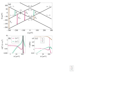
Figure 2: (a) Spectrum of $H_{d}$ [Eq. (1)] as a function of detuning $\epsilon$ for the case $t\ll\Omega_{z},$ in the presence of spin-orbit coupling ($\mathbf{K}_{\mathrm{so}}\neq\mathbf{0},$ $\mathbf{K}_{\mathrm{nuc}}=\mathbf{0}$). Correspondence with the eigenstates of $H_{0}$ [Eqs. (2) and (5)] is indicated for relevant regions of the spectrum. Avoided crossings due to spin-orbit coupling occur at $\epsilon\approx\pm\Omega_{z}$. The spectrum shown corresponds to $t=10\ \mu\mbox{eV}$ Sup , $B=6.5\ \mbox{T}$ Nowack et al. (2011); Sup , the dot size $\sigma=15\ \mbox{nm}$ and interdot separation $a=110\ \mbox{nm},$ the GaAs effective mass $m^{*}=0.067m_{e}$ (where $m_{e}$ is the free-electron mass) and g-factor $g=0.36$, the Rashba and linear Dresselhaus spin-orbit strengths $\alpha_{0}=3.3\times 10^{-12}\ \mbox{eV$\cdot$m}$ and $\beta_{0}=4.5\times 10^{-12}\ \mbox{eV$\cdot$m}$, respectively, and $\theta=\pi/8.$ The values of $\alpha_{0},$ $\beta_{0},$ and $\theta$ are used to determine $\mathbf{K}_{\mathrm{so}}=\left(r,s,q\right).$ (b) Dipole-dependent factors $\langle|d_{b}|^{2}\rangle$ and $\langle|d_{e}|^{2}\rangle$ [Eqs. (8) and (9)] used to qualitatively model the relaxation rates $\Gamma_{b}$ and $\Gamma_{e}$ in (a), as a function of detuning for $B_{\mathrm{nuc}}=0$ (solid lines) and $B_{\mathrm{nuc}}=3\ \mathrm{mT}$ (dotted lines), with $\alpha_{0}=3.3\times 10^{-14}\ \mbox{eV$\cdot$m}$ and $\beta_{0}=4.5\times 10^{-14}\ \mbox{eV$\cdot$m}$. All other parameters are identical to those used in (a). Units for the dipole are given in terms of the Bohr radius $a_{0}.$ The dipole model is not valid in the shaded region. (c) Relaxation rates $\Gamma_{a},$ $\Gamma_{b},$ and $\Gamma_{e}$ as a function of detuning. The rates are calculated using $\rho_{0}=5.3\times 10^{3}\ \mbox{kg/m}^{3},$ $c_{l}=5.3\times 10^{3}\ \mathrm{m}/\mathrm{s},$ $c_{t}=2.5\times 10^{3}\ \mathrm{m}/\mathrm{s},$ $\beta_{l}=7.0\ \mbox{eV},$ and $\Xi=1.4\times 10^{9}\ \mbox{eV/m}$ Stano and Fabian (2006), together with the parameter values used in (b). Lines are guides to the eye.

We approximate the relaxation rates $\Gamma_{b}$ and $\Gamma_{e}$ [Fig. 2(a)] in the presence of both $H_{\mathrm{so}}$ and $H_{\mathrm{nuc}}$ by calculating the first-order terms $d_{b}$ and $d_{e}$ of the dipole matrix elements $\tilde{\left\langle-,\uparrow\right|}D\tilde{\left|-,\downarrow\right\rangle}$ and $\tilde{\left\langle+,\uparrow\right|}D\tilde{\left|-,\downarrow\right\rangle}$, respectively. These terms are functions of the spin-flipping components $r,\ s,\ u,$ and $v$ in Eqs. (3) and (4). Averaging over the nuclear field distribution Merkulov et al. (2002); Erlingsson and Nazarov (2002); Johnson et al. (2005); Taylor et al. (2007)

$$P\left(\mathbf{K}_{\mathrm{nuc}}\right) = \frac{1}{\left(2\pi b_{\mathrm{nuc}}^{2}\right)^{3/2}}\exp\left(-\frac{\left|\mathbf{K}_{\mathrm{nuc}}\right|^{2}}{2b_{\mathrm{nuc}}^{2}}\right),$$ (7)

where $b_{\mathrm{nuc}}\equiv\left|g\right|\mu_{B}B_{\mathrm{nuc}}=\sqrt{\langle\left|\mathbf{K}_{\mathrm{nuc}}\right|^{2}\rangle/3},$ gives $\langle u\rangle=\langle v\rangle=0$ and $\langle u^{2}\rangle=\langle v^{2}\rangle=b_{\mathrm{nuc}}^{2}.$ We thus find

$$\langle|d_{b}|^{2}\rangle = \left[\frac{ea}{2}\left(\frac{2t}{\Delta}\right)\frac{\Omega_{z}}{(\Delta-\Omega_{z})(\Delta+\Omega_{z})}\right]^{2}\chi,$$ (8)

$$\langle|d_{e}|^{2}\rangle = \left[\frac{ea}{2}\left(\frac{\epsilon}{\Delta}\right)\frac{1}{\Delta-\Omega_{z}}\right]^{2}\chi,$$ (9)

$$\chi \equiv \left[r^{2}+s^{2}+\left(\frac{2t}{\Omega_{z}}\right)^{2}\left(2b_{\mathrm{nuc}}^{2}\right)\right].$$

These expressions are plotted in Fig. 2(b). Note that both Eqs. (8) and (9) are undefined at the avoided crossing points in Fig. 2(a), where $\Delta=\Omega_{z}$. Thus, the curves shown in Fig. 2(b) are valid only away from these points (i.e., where nondegenerate perturbation theory is a reasonable approximation). Both $\langle|d_{b}|^{2}\rangle$ and $\langle|d_{e}|^{2}\rangle$ are only slightly modified by the coupling of the electron spin to an effective nuclear field of rms strength $B_{\mathrm{nuc}}=3\ \mathrm{mT}$ Johnson et al. (2005), as expected from Eqs. (8) and (9) in which the nuclear field term is scaled with respect to the spin-orbit terms by a factor $\left(2t/\Omega_{z}\right)^{2}\ll 1$ Schreiber et al. (2011). Saturation of $\langle|d_{b}|^{2}\rangle$ occurs at zero detuning for both the $B_{\mathrm{nuc}}=0$ and the $B_{\mathrm{nuc}}=3\ \mathrm{mT}$ cases. On the other hand, $\langle|d_{e}|^{2}\rangle$ vanishes at $\epsilon=0$ regardless of the value of $B_{\mathrm{nuc}}$. As the experimental relaxation rate contains a local minimum at zero detuning (see Fig. 3), the present analysis suggests that the direct transition $\tilde{\left|-,\downarrow\right\rangle}\rightarrow\tilde{\left|-,\uparrow\right\rangle}$ alone does not account for the observed spin relaxation and that indirect relaxation via the excited state $\tilde{\left|+,\uparrow\right\rangle}$ potentially plays a significant role in the spin-flip rate. The relative contributions of the direct and indirect transitions to the overall rate are explored in Sup .

To compare our theoretical predictions more directly with the experimental results, we carry out the full calculation of the relaxation rates for both direct and indirect transitions to the ground state by applying Fermi’s golden rule to relaxation induced by $H_{\mathrm{ep}}$ [Eq. (6)]. Details are given in the Supplemental Material Sup . We set $\mathbf{K}_{\mathrm{nuc}}=0$ for simplicity, as the preceding analysis based on dipole matrix elements suggests that the hyperfine term $H_{\mathrm{nuc}}$ represents only a small correction to the decay rate [see Eqs. (8), (9) and Fig. 2(b)]. Application of a Schrieffer-Wolff transformation Schrieffer and Wolff (1966) enables diagonalization of the full double-dot Hamiltonian $H_{d}$ for all $\epsilon,$ including the avoided crossing points $\epsilon\approx\pm\Omega_{z}$, and the eigenstates of $H_{d}$ are used to calculate the relaxation rates via Eqs. (S1)-(S3) Sup .

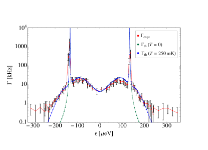
Figure 3: Experimental detuning-dependent single-spin relaxation rate $\left(\Gamma_{\mathrm{expt}}\right)$ and comparison with the toy model described in the present work $\left(\Gamma_{\mathrm{th}}\right)$ for both zero and finite temperature. Error bars depict 90% confidence intervals for the data. The parameter values used to calculate $\Gamma_{\mathrm{th}}$ are the same as those used in (b) and (c) of Fig. 2.

Relevant portions of the curves for the decay rates $\Gamma_{21},$ $\Gamma_{31},$ and $\Gamma_{32}$ (where we number the levels according to their energy eigenvalues and use $\Gamma_{if}$ to denote the rate of relaxation from level $i$ to level $f$) are plotted together in Fig. 2(c). The rate $\Gamma_{a}$ is associated with mainly charge relaxation and is given by $\Gamma_{21}$ ($\Gamma_{31}$) for $\left|\epsilon\right|\lesssim\Omega_{z}$ ($\left|\epsilon\right|\gtrsim\Omega_{z}$), while $\Gamma_{b}$ is associated with mainly spin relaxation and is given by $\Gamma_{31}$ ($\Gamma_{21}$) for $\left|\epsilon\right|\lesssim\Omega_{z}$ ($\left|\epsilon\right|\gtrsim\Omega_{z}$). The rate $\Gamma_{e}$ corresponds to a combination of spin and charge relaxation and is given by $\Gamma_{32}$ for all $\left|\epsilon\right|$. Note that $\Gamma_{a}\gg\Gamma_{e},$ which is consistent with our prior assumption that the effective rate for indirect relaxation to the ground state is determined by $\Gamma_{e}$.

For $\left|\epsilon\right|\lesssim\Omega_{z},$ indirect spin relaxation occurs by a transition to the lower-energy intermediate state via phonon emission [Fig. 2(a)]. On the other hand, the indirect transition for $\left|\epsilon\right|\gtrsim\Omega_{z}$ requires phonon absorption in order to excite the electron to the higher-energy intermediate state. Using the Einstein coefficients and the Bose-Einstein distribution $\left\langle n\right\rangle=1/\left[\exp\left(\Delta_{d}/k_{B}T\right)-1\right]$ (where $k_{B}$ is the Boltzmann constant and $T$ is the temperature) to express the rates of spontaneous emission, stimulated emission, and absorption associated with the lowest three double-dot levels in Fig. 2(a) in terms of $\Gamma_{a},$ $\Gamma_{b},$ and $\Gamma_{e}$ Fujisawa et al. (1998), we take the full theoretical detuning-dependent spin relaxation rate $\Gamma_{\mathrm{th}}$ to be given by $\Gamma_{b}+\Gamma_{e}$ for $\left|\epsilon\right|\lesssim\Omega_{z}$ and by $\Gamma_{b}+\Gamma_{e}\left\langle n\right\rangle/\left(\left\langle n\right\rangle+1\right)$ for $\left|\epsilon\right|\gtrsim\Omega_{z}.$ This rate is plotted together with the zero-temperature limit of the model and the measured rate $\Gamma_{\mathrm{expt}}$ in Fig. 3 for $T=250\ \mathrm{mK}$ Sup ; Nowack et al. (2011). At the avoided crossings associated with spin-orbit coupling ($\epsilon\approx\pm\Omega_{z}$), we find peaks in $\Gamma_{\mathrm{th}}$ that resemble the spin hot spot peaks observed experimentally. The zero-detuning minimum found in the measurements appears in both the zero-and the finite-temperature models. In addition, close qualitative agreement between the finite-temperature model and experiment is observed for a wide range of detuning values. While limitations of our theoretical description arise from the two-level approximation we use for the orbital states, we have nevertheless shown that several characteristic features present in the measured detuning dependence of the double-dot spin relaxation rate can be understood within this simple model.

The results of the present work therefore suggest that, in accordance with the case of single lateral GaAs quantum dots Amasha et al. (2008), the observed variation of the spin relaxation rate with detuning in double dots is dominated by spin-orbit mediated electron-phonon coupling. The spin-orbit interaction may thus provide the key to rapid all-electrical initialization of single spins.

Note added. During the preparation of this manuscript, we became aware of a recent experimental observation of a spin hot spot in a Si quantum dot Yang et al. .

We thank N. M. Zimmerman, M. D. Stiles, and P. Stano for helpful comments. Research was supported by DARPA MTO, the Office of the Director of National Intelligence, Intelligence Advanced Research Projects Activity (IARPA), through the Army Research Office (Grant W911NF-12-1-0354), SOLID (EU), and an ERC Starting Grant.

References

- Loss and DiVincenzo (1998) D. Loss and D. P. DiVincenzo, Phys. Rev. A 57, 120 (1998).
- Hanson et al. (2007) R. Hanson, L. P. Kouwenhoven, J. R. Petta, S. Tarucha, and L. M. K. Vandersypen, Rev. Mod. Phys. 79, 1217 (2007).
- Hanson and Awschalom (2008) R. Hanson and D. D. Awschalom, Nature 453, 1043 (2008).
- Taylor et al. (2008) J. M. Taylor, P. Cappellaro, L. Childress, L. Jiang, D. Budker, P. R. Hemmer, A. Yacoby, R. Walsworth, and M. D. Lukin, Nature Phys. 4, 810 (2008).
- Dolde et al. (2011) F. Dolde, H. Fedder, M. W. Doherty, T. Nobauer, F. Rempp, G. Balasubramanian, T. Wolf, F. Reinhard, L. C. L. Hollenberg, F. Jelezko, and J. Wrachtrup, Nature Phys. 7, 459 (2011).
- Kato et al. (2003) Y. Kato, R. C. Myers, D. C. Driscoll, A. C. Gossard, J. Levy, and D. D. Awschalom, Science 299, 1201 (2003).
- Rashba and Efros (2003) E. I. Rashba and A. L. Efros, Phys. Rev. Lett. 91, 126405 (2003).
- Taylor et al. (2005) J. M. Taylor, H. A. Engel, W. Dur, A. Yacoby, C. M. Marcus, P. Zoller, and M. D. Lukin, Nature Phys. 1, 177 (2005).
- Tokura et al. (2006) Y. Tokura, W. G. van der Wiel, T. Obata, and S. Tarucha, Phys. Rev. Lett. 96, 047202 (2006).
- Nowack et al. (2007) K. C. Nowack, F. H. L. Koppens, Y. V. Nazarov, and L. M. K. Vandersypen, Science 318, 1430 (2007).
- Laird et al. (2007) E. A. Laird, C. Barthel, E. I. Rashba, C. M. Marcus, M. P. Hanson, and A. C. Gossard, Phys. Rev. Lett. 99, 246601 (2007).
- Pioro-Ladriere et al. (2008) M. Pioro-Ladriere, T. Obata, Y. Tokura, Y. S. Shin, T. Kubo, K. Yoshida, T. Taniyama, and S. Tarucha, Nature Phys. 4, 776 (2008).
- Schreiber et al. (2011) L. R. Schreiber, F. R. Braakman, T. Meunier, V. Calado, J. Danon, J. M. Taylor, W. Wegscheider, and L. M. K. Vandersypen, Nat. Commun. 2, 556 (2011).
- Shafiei et al. (2013) M. Shafiei, K. C. Nowack, C. Reichl, W. Wegscheider, and L. M. K. Vandersypen, Phys. Rev. Lett. 110, 107601 (2013).
- Khaetskii and Nazarov (2000) A. V. Khaetskii and Y. V. Nazarov, Phys. Rev. B 61, 12639 (2000).
- Khaetskii and Nazarov (2001) A. V. Khaetskii and Y. V. Nazarov, Phys. Rev. B 64, 125316 (2001).
- Golovach et al. (2004) V. N. Golovach, A. Khaetskii, and D. Loss, Phys. Rev. Lett. 93, 016601 (2004).
- Bulaev and Loss (2005) D. V. Bulaev and D. Loss, Phys. Rev. B 71, 205324 (2005).
- Stano and Fabian (2005) P. Stano and J. Fabian, Phys. Rev. B 72, 155410 (2005).
- Stano and Fabian (2006) P. Stano and J. Fabian, Phys. Rev. Lett. 96, 186602 (2006).
- Amasha et al. (2008) S. Amasha, K. MacLean, I. P. Radu, D. M. Zumbühl, M. A. Kastner, M. P. Hanson, and A. C. Gossard, Physical Review Letters 100, 046803 (2008).
- Erlingsson et al. (2001) S. I. Erlingsson, Y. V. Nazarov, and V. I. Fal’ko, Phys. Rev. B 64, 195306 (2001).
- Erlingsson and Nazarov (2002) S. I. Erlingsson and Y. V. Nazarov, Phys. Rev. B 66, 155327 (2002).
- Merkulov et al. (2002) I. A. Merkulov, A. L. Efros, and M. Rosen, Phys. Rev. B 65, 205309 (2002).
- Johnson et al. (2005) A. C. Johnson, J. R. Petta, J. M. Taylor, A. Yacoby, M. D. Lukin, C. M. Marcus, M. P. Hanson, and A. C. Gossard, Nature 435, 925 (2005).
- Koppens et al. (2005) F. H. L. Koppens, J. A. Folk, J. M. Elzerman, R. Hanson, L. H. W. van Beveren, I. T. Vink, H. P. Tranitz, W. Wegscheider, L. P. Kouwenhoven, and L. M. K. Vandersypen, Science 309, 1346 (2005).
- Taylor et al. (2007) J. M. Taylor, J. R. Petta, A. C. Johnson, A. Yacoby, C. M. Marcus, and M. D. Lukin, Phys. Rev. B 76, 035315 (2007).
- van der Wiel et al. (2002) W. G. van der Wiel, S. De Franceschi, J. M. Elzerman, T. Fujisawa, S. Tarucha, and L. P. Kouwenhoven, Rev. Mod. Phys. 75, 1 (2002).
- Hayashi et al. (2003) T. Hayashi, T. Fujisawa, H. D. Cheong, Y. H. Jeong, and Y. Hirayama, Phys. Rev. Lett. 91, 226804 (2003).
- Petta et al. (2004) J. R. Petta, A. C. Johnson, C. M. Marcus, M. P. Hanson, and A. C. Gossard, Phys. Rev. Lett. 93, 186802 (2004).
- Gorman et al. (2005) J. Gorman, D. G. Hasko, and D. A. Williams, Phys. Rev. Lett. 95, 090502 (2005).
- Fujisawa et al. (1998) T. Fujisawa, T. H. Oosterkamp, W. G. van der Wiel, B. W. Broer, R. Aguado, S. Tarucha, and L. P. Kouwenhoven, Science 282, 932 (1998).
- Raith et al. (2012) M. Raith, P. Stano, F. Baruffa, and J. Fabian, Phys. Rev. Lett. 108, 246602 (2012).
- Wang and Wu (2006) Y. Y. Wang and M. W. Wu, Phys. Rev. B 74, 165312 (2006).
- Wang et al. (2011) M. Wang, Y. Yin, and M. W. Wu, J. Appl. Phys. 109, 103713 (2011).
- Fabian and Das Sarma (1998) J. Fabian and S. Das Sarma, Physical Review Letters 81, 5624 (1998).
- Raith et al. (2011) M. Raith, P. Stano, and J. Fabian, Phys. Rev. B 83, 195318 (2011).
- Rashba (1960) E. I. Rashba, Sov. Phys. Solid State 2, 1109 (1960).
- Bychkov and Rashba (1984) Y. A. Bychkov and E. I. Rashba, J. Phys. C 17, 6039 (1984).
- Dresselhaus (1955) G. Dresselhaus, Phys. Rev. 100, 580 (1955).
- (41) Note that implicitly includes the homogeneous part of the nuclear field.
- (42) See Supplemental Material.
- Elzerman et al. (2004) J. M. Elzerman, R. Hanson, L. H. Willems van Beveren, B. Witkamp, L. M. K. Vandersypen, and L. P. Kouwenhoven, Nature 430, 431 (2004).
- Nowack et al. (2011) K. C. Nowack, M. Shafiei, M. Laforest, G. E. D. K. Prawiroatmodjo, L. R. Schreiber, C. Reichl, W. Wegscheider, and L. M. K. Vandersypen, Science 333, 1269 (2011).
- Mahan (1990) G. Mahan, Many-Particle Physics (Plenum, 1990).
- Fujisawa et al. (2001) T. Fujisawa, Y. Tokura, and Y. Hirayama, Phys. Rev. B 63, 081304 (2001).
- Schrieffer and Wolff (1966) J. R. Schrieffer and P. A. Wolff, Physical Review 149, 491 (1966).
- (48) C. H. Yang, A. Rossi, R. Ruskov, N. S. Lai, F. A. Mohiyaddin, S. Lee, C. Tahan, G. Klimeck, A. Morello, and A. S. Dzurak, arXiv:1302.0983v1 .