Watersheds on edge or node weighted graphs "par l’exemple"

Abstract

Watersheds have been defined both for node and edge weighted graphs. We show that they are identical: for each edge (resp. node) weighted graph exists a node (resp. edge) weighted graph with the same minima and catchment basin.

1 Introduction

The watershed is a versatile and powerful segmentation tool. Its use for segmentation is due to Ch.Lantuéjoul and S.Beucher [2]. It may be applied on an image considered as a topographic surface [2], [9], [2]. An image may be considered as a node weighted graph ; the nodes are the pixels of the image, weighted by their grey tone ; the edges connect neighboring nodes and are not weighted. . Or the watershed may be applied on an edge weighted graph, such as a region adjacency graph [4], where the nodes are unweighted and represent the catchment basins, and the edges connecting neighboring basins are weighted by the altitude of the pass point separating two basins.

In the first case, one has to find the watershed on a node weighted graphs, in the second on an edge weighted graph [5]. Definitions and algorithms are not the same in both worlds, although the have the same physical inspirations. The rain model, where the destiny of a drop of water falling on the surface defines the catchment basins ; a catchment basin is the attraction zone of a minimum, i.e. the set of nodes from where a drop of water may reach this minimum. Catchment basins generally overlap.The flooding model where the relief is flooded from sources placed at the regional minima and meet for forming a partition. The later method being often implemented as shortest distance algorithms [10], [11]. There is no opposition between these models as the same trajectory may be followed from bottom to top, and we have a flooding model or from top to bottom and we have a rain model. A good review on the watershed may be found in [13], and in the recent book [12].

This paper aims at showing the equivalence between edge or node weighted graphs for the construction of the watershed.

2 Graphs

2.1 General definitions

A non oriented graph $G=\left[N,E\right]$ is a collection $N$ of vertices or nodes and of edges $E,$ an edge $u\in E$ being a pair of vertices (see [1],[6]).

A chain of length $n$ is a sequence of $n$ edges $L=\left\{e_{1},e_{2,}\ldots,e_{n}\right\}$, such that each edge $e_{i}$ of the sequence $\left(2\leq i\leq n-1\right)$ shares one extremity with the edge $e_{i-1}$ $(e_{i-1}\neq e_{i})$, and the other extremity with $e_{i+1}$ $(e_{i+1}\neq e_{i})$.

A path between two nodes $x$ and $y$ is a sequence of nodes $(n_{1}=x,n_{2},...,n_{k}=y)$ such that two successive nodes $n_{i}$ and $n_{i+1}$ are linked by an edge.

A cycle is a chain or a path whose extremities coincide.

A cocycle is the set of all edges with one extremity in a subset $Y$ and the other in the complementary set $\overline{Y}.$

The subgraph spanning a set $A\subset N$ is the graph $G_{A}=[A,E_{A}]$, where $E_{A}$ are the edges linking two nodes of $A.$

The partial graph associated to the edges $E^{\prime}\subset E$ is $G^{\prime}=[N,E^{\prime}].$

A connected graph is a graph where each pair of nodes is connected by a path.

2.2 Weighted graphs: regional minima and catchment basins

In a graph $G=\left[N,E\right],$ edges and nodes may be weighted : $e_{ij}$ is the weight of the edge $(i,j)$ and $n_{i}$ the weight of the node $i.$ The weights take their value in the completely ordered lattice $\mathcal{T}$.

2.2.1 Edge weighted graphs

Regional minima

A subgraph $G^{\prime}$ of an edge weighted graph $G$ is a flat zone, if any two nodes of $G^{\prime}$ are connected by a chain of uniform altitude.

A subgraph $G^{\prime}$ of a graph $G$ is a regional minimum if $G^{\prime}$ is a flat zone and all edges in its cocycle have a higher altitude.

Catchment basins

A chain $L=\left\{e_{1},e_{2,}\ldots,e_{n}\right\}$ is a flooding chain, if each edge $e_{k}=(n_{k},n_{k+1})$ is one of the lowest edges of its extremity $n_{k},$ and if along the chain the weigths of the edges is never increasing.

Definition 1

The catchment basin of a minimum $m$ is the set of nodes linked by a flooding chain with a node within $m.\$

2.2.2 Node weighted graphs

Regional minima

A subgraph $G^{\prime}$ of a node weighted graph $G$ is a flat zone, if any two nodes of $G^{\prime}$ are connected by a path along which all nodes have the same altitude.

A subgraph $G^{\prime}$ of a graph $G$ is a regional minimum if $G^{\prime}$ is a flat zone and all neighboring nodes have a higher altitude.

Catchment basins

A flooding path between two nodes is a path along which the weigths of the nodes is never increasing.

Definition 2

The catchment basin of a minimum $m$ is the set of nodes linked by a non ascending path with a node within $m.\$

Remark 1

The definition of the catchment basins is the loosest possible, compatible with the physical inspiration of the rain model : a drop of water falling on a surface cannot go upwards. With this definition, the same node may belong to various catchment basins. In other words there are large overlapping zones of the catchment basins. As most algorithm aim at producing a partition, they propose various methods for suppressing these overlapping zones.

3 Outline of the method

We want to show the equivalence of the watershed on node and edge weighted graphs. We first present the outline of the method on the two simple graphs in fig.1, the left one being edge weighted and the right being node weighted.

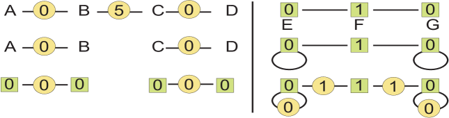
Figure 1: On the left an edge weighted graph transformed into a flooding graph. On the right a node weighted graph transformed into a flooding graph. 

Consider first the edge weighted graph. It has 4 nodes A,B,C and  D separated by weighted edges. In a flooding chain, each node is linked with the next node by one of its lowest edges. For this reason, if an edge is not the lowest edge of one of its extremities, it will never be crossed by a flooding chain. It is the case for the edge BC: the lowest adjacent edge of B is AB and the lowest adjacent edge of  C is CD. For this reason, this edge BC can be suppressed from the graph (as presented in the second line), without modifying the flooding chains of the original graph. In a last step we assign weights to the nodes: each node gets the weight of its lowest adjacent edge, as represented in the third line .he resulting graph is called flooding graph. In our case, it has two regional minima, which are identical if one considers them from the point of view of the edge weights or the node weights. For this simple graph, they constitute the catchment basins.

Consider now the node weigthed graph on the right of fig.1 . It has two isolated regional minima. One adds a loop edge linking each isolated node with itself as shown in fig.1. This modification does not change the flooding paths of the initial graph. The last step consists in assigning, as weight to each edge, the maximal weight of its extremities. The added loops algo get an edge weight. As a result we get again a flooding graph with the following features:

• the edges spanning the regional minima of the node weighted graph are the regional minima of the edge weighted graph.

• the lowest adjacent edge of a node has the same weight as this node. For this reason each flooding path of the node weighted graph is simultaneously a flooding chain of the edge weighted graph.

Having an identity between the minima and between flooding paths and chains, the catchment basins of both graphs are the same. In our case we have two basins with an overlapping zone containing the node F.

4 The flooding graph

4.1 The flooding adjunction

We define two operators between edges and nodes :
- an erosion $\left[\varepsilon_{en}n\right]_{ij}=n_{i}\wedge n_{j}$ and its adjunct dilation $\left[\delta_{ne}e\right]_{i}=\underset{(k\text{\thinspace neighbors\thinspace of\thinspace}\,i)}{\bigvee e_{ik}}$
- a dilation $\left[\delta_{en}n\right]_{ij}=n_{i}\vee n_{j}$ and its adjunct erosion $\left[\varepsilon_{ne}e\right]_{i}=\underset{(k\text{\thinspace neighbors\thinspace of\thinspace}\,i)}{\bigwedge e_{ik}}$

The pairs $(\varepsilon_{ne},\delta_{en})$ and $(\varepsilon_{en},\delta_{ne})$ are adjunct operators. The pairs $(\varepsilon_{ne},\delta_{ne})$ and $(\varepsilon_{en},\delta_{en})$ dual operators.

We call the first pair flooding adjunction as we may give it a physical explanation. Let us consider a region adjacency graph of a topographical surface, where $n_{i}$ and $n_{j}$ represent the flood level in the basins $i$ and $j,$ and $e_{ij}$ represents the altitude of the pass pont between both basins. Then:
* the altitudes of the nodes $i$ and $j,$ the lowest flood covering $i$ and $j$ has the altitude $\left[\delta_{en}n\right]_{ij}=n_{i}\vee n_{j}$
* if $i$ represents a catchment basin, $e_{ik}$ the altitude of the pass points with the neighboring basin $k,$ then the highest level of flooding without overflow through an adjacent edge is $\left[\varepsilon_{ne}e\right]_{i}=\underset{(k\text{\thinspace neighbors\thinspace of\thinspace}\,i)}{\bigwedge e_{ik}}.$

As $\varepsilon_{ne}$ and $\delta_{en}$ are adjunct operators, the operator $\varphi_{n}=\varepsilon_{ne}\delta_{en}$ is a closing on $n$ and $\gamma_{e}=\delta_{en}\varepsilon_{ne}$ is an opening on $e$.

4.2 The opening $\gamma_{e}$

We consider first an edge weighted graph $G_{e}$ and study the effect of the opening $\gamma_{e}$ on its edge weights. Fig.2 presents from left to right: 1) an edge weighted graph, , 2) the result of the erosion $\varepsilon_{ne}$, 3) the subsequent dilation producing an opening. The edges in red are those whose weight has been reduced by the opening. The others, invariant by the opening $\gamma_{e}$ are the edges which are, as we establish below, the lowest edge of one of their extremities. Two possibilities exist for an edge $(i,j)$ with a weight $\lambda:$
* the edge $(i,j)$ has lower neighboring edges at each extremity. Hence $\varepsilon_{ne}(i)<\lambda$ and $\varepsilon_{ne}(j)<\lambda$ ; hence $\gamma_{e}=\delta_{en}\varepsilon_{ne}(i,j)=\varepsilon_{en}(i)\vee\varepsilon_{en}(j)<\lambda:$ the edge $(i,j)$ is not invariant by the opening $\gamma_{e}$
* the edge $(i,j)$ is the lowest edge of the extremity $i.$ Then $\varepsilon_{ne}(i)=\lambda$ and $\varepsilon_{ne}(j)\leq\lambda$ ; hence $\gamma_{e}=\delta_{en}\varepsilon_{ne}(i,j)=\varepsilon_{en}(i)\vee\varepsilon_{en}(j)=\lambda:$ the edge $(i,j)$ is invariant by the opening $\gamma_{e}$

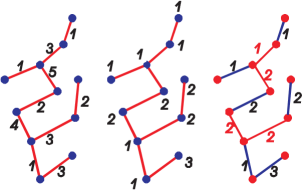
Figure 2: From left to right: 1) an edge weighted graph, in the centre, 2) the result of the erosion $\varepsilon_{ne}$, 3) the subsequent dilation produces an opening. The edges in red are those whose weight has been reduced by the opening as they were not the lowest edge of one of their extremities in the initial distribution of edge weights.

Hence the edges which are invariant by $\gamma_{e}$ are all edges which are the lowest edges for one of their extremities. The operator keeping for each node only its lowest adjacent edges is written $\downarrow\ :G\rightarrow\ \downarrow G.\$As each node has at least one lowest neighboring edge, the resulting graph $\downarrow G$ spans all the nodes. The resulting graph also contains all flooding chains of the initial graph (since in a flooding chain, each edge is the lowest edge of one of its extremities).

4.2.1 The regional minima of a graph $G_{e}$ invariant by the opening $\gamma_{e}$

Consider an edge weighted graph $G_{e}$ invariant by the opening $\gamma_{e}.$ We assign to the nodes the weights $\varepsilon_{ne}.\$We call $G_{n}$ the graph on which one only considers the node weights.

Theorem 4.1

If an edge weighted graph $G_{e}$ is invariant by the opening $\gamma_{e},$ then its regional minima edges span the regional minima nodes of $G_{n}.$

Proof: A regional minimum $m$ of the graph $G_{e}$ is a plateau of edges with altitude $\lambda$, with all adjacent edges in the cocycle having a weight higher than $\lambda.\$If a node $i$ belongs to this regional minimum, its adjacent edges have a weight $\geq\lambda$ but it has at least one neighboring edge with weight $\lambda$ : hence the weight of $i$ is $\left(\varepsilon_{ne}e\right)_{i}=\lambda.$ Consider now an edge $(s,t),$ with $s$ inside the regional minimum and $t$ outside. Then $e_{st}>\lambda$. As $G\$is invariant by $\gamma_{e},$ the edge $(s,t)$ is one of the lowest edges of the nodes $t$ : thus the weight of $t$ is $\left(\varepsilon_{ne}e\right)_{t}=e_{st}>\lambda.\$This shows that the nodes spanned by the regional minimum $m$ form a regional minimum of the graph $G_{n}.$

4.3 The closing $\varphi_{n}$

Consider now a node weighted graph $G.\$The closing $\varphi_{n}$ is obtained by a dilation $\delta_{en}$ of the node weights followed by an erosion $\varepsilon_{ne}.\$

Lemma 1

The closing $\varphi_{n}$ replaces each isolated node constituting a regional minimum by its lowest neighboring node and leaves all other nodes unchanged.

Proof

Consider a node with a weight $\lambda$ belonging to a regional minimum:
* consider the case where the node $i$ is an isolated regional minimum. Then $\delta_{en}$ assigns to all edges adjacent to $i$ a weight bigger than $\lambda.\$The subsequent erosion $\varepsilon_{ne}$ assigns to $i$ the smallest of these weights, which is the weight of the smallest neighbor. The node $i$ is not invariant by the closing $\varphi_{n}.$
* Suppose that $i$ belongs to a regional minimum which is not isolated. The dilation $\delta_{en}$ assigns to each edge adjacent to $i$ a weight $\geq\lambda.\$If $i$ has a a neighbor $j$ with a weight $\mu\leq\lambda,.$then $\delta_{en}$ assigns to the edge $(i,j)$ the weight $\lambda.\$The subsequent erosion $\varepsilon_{ne}$ assigns to $i$ the smallest of these weights, that is $\lambda.$ The node $i$ is invariant by the closing $\varphi_{n}.$

Hence if $G$ has isolated regional minima, it is not invariant by $\varphi_{n}.\$If we add a loop edge linking each isolated regional minimum with itself we obtain a graph invariant by $\varphi_{n}.\$Indeed, if $i$ is an isolated regional minimum with weight $\lambda,$ we add a loop edge $(i,i)$ ; the dilation $\delta_{en}$ assigns to the loop the weight $\lambda$ and to all other edges adjacent to $i,$ a weight $>\lambda.\$The subsequent erosion $\varepsilon_{ne}$ assigns to $i$ the smallest of these weights, which is the weight of the loop, i.e. $\lambda.$

We write $\circlearrowright:G\rightarrow\ \circlearrowright G$ the operator which adds to a node weighted graph a loop between each isolated regional minimum and itself.

4.3.1 The regional minima of a graph $G_{n}$ invariant by the closing $\varphi_{n}$

Consider a node weighted graph $G_{n}$ invariant by the closing $\varphi_{n}.$ We assign to the edges the weights $\delta_{en}.\$We call $G_{e}$ the graph on which one only consider the edge weights.

Theorem 4.2

If $G$ is invariant by the closing $\varphi_{n},$ then the edges spanning the regional minima nodes of $G_{n}$ form the regional minima edges of $G_{e}.$

Proof: A regional minimum $m$ of $G_{n}$ is a plateau of pixels with altitude $\lambda$, containing at least two nodes (there are no isolated regional minima as $G_{n}$ is invariant by $\varphi_{n}$). All internal edges of the plateau get the valuation $\lambda$ by $\delta_{en}n.$ If an edge $(i,j)$ has the extremity $i$ in the minimum and the extremity $j$ outside, then $\delta_{en}n(i,j)>\lambda.\$Hence, for the graph $G_{e},$ the edges spanning the nodes of $m$ form a regional minimum.

4.4 The flooding graph

We consider now a graph $\ G$ on which both nodes and edges are weighted. If we consider only the edge weights we write $G_{e}$ and $G_{n}$ if we consider only the node weights.

Definition: An edge and node weighted graph $G=[N,E]$ is a flooding graph iff its weight distribution $(n,e)$ verifies both $\delta_{en}n=e$ and $\varepsilon_{ne}e=n.$

In a flooding graph, the weight distribution $(n,e)$ verifies $e=\delta_{en}n=\delta_{en}\varepsilon_{ne}e\newline =\gamma_{e}e$ and $n=\varepsilon_{ne}e=\varepsilon_{ne}\delta_{en}n=\varphi_{n}n$ showing that $n\in\operatorname*{Inv}(\varphi_{n})$ and $e\in\operatorname*{Inv}(\gamma_{e}).$

As $G$ is invariant by $\gamma_{e},$ all its edges are the lowest edge of one of their extremities. And as $G$ is invariant by $\varphi_{n},$ it has no isolated regional minimum.

We have established earlier that:

• if a graph $G_{e}$ is invariant by $\gamma_{e},$ then its regional minima edges span the regional minima nodes of $G_{n}.\$

• if a graph $G_{n}$ is invariant by $\varphi_{n},$ then the edges spanning the regional minima nodes of $G_{n}$ form the regional minima edges of $G_{e}.$

As a flooding graph is both invariant by $\gamma_{e}$ and by $\varphi_{n},$ we get the following theorem.

Theorem 4.3

If $G$ is a flooding graph then the node weighted graph $G_{n}$ and the edge weighted graph $G_{e}$ have the same regional minima subgraph. More precisely, the regional minima nodes of $G_{n}$ are spanned by the regional minima edges of $G_{e}.$

Fig.3 presents the same flooding graph, on the left with its edge weights and on the right with its node weights : they have exactly the same regional minima.

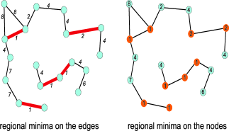
Figure 3: Whether one consider the egde weights or the node weights produces the same regional minima. 

4.4.1 Flooding paths and flooding chains

Consider a flooding path on $G_{n},$ i.e. a path $(n_{1},n_{2},...n_{k})$ of neighboring nodes with a non increasing weight, starting at node $n_{1}$ and ending at node $n_{k}$ belonging to a regional minimum of $G_{n}$. As $n_{i}\geq n_{i+1}$, the weight of the edge $\left(n_{i},n_{i+1}\right)$ obtained by $\delta_{en}$ is equal to the weight of $n_{i}$ and is one of teh lowest edges of $n_{i}.$ This shows, that the series of edges $\left(n_{i},n_{i+1}\right)$ form a flooding chain of $G_{e}$, ending in a regional minimum of $G_{e}.\$

Inversely, consider a flooding chain$[(n_{1},n_{2}),(n_{2},n_{3}),...(n_{k-1},n_{k})]$ of $G_{e}.$ The weights of the edges are not increasing. Furthermore, the edge $\left(n_{i},n_{i+1}\right)$ is the lowest edge of the node $n_{i}$. As in a flooding graph the lowest edge of a node has the same weight than this node, the edge $\left(n_{i},n_{i+1}\right)$ has the same weight than the node $n_{i}.\$Thus the path $(n_{1},n_{2},...n_{k})$ also is a flooding path of $G_{n}$ ending a regional minimum of $G_{n}.$

There is a one to one correspondance between the regional minima of $G_{e}$ and $G_{n}$ ; there is also a one to one correspondance between the flooding paths and the flooding tracks, with the same weight distribution. This shows that both graphs, $G_{e}$ on which we only consider the edge weights and $G_{n}$ on which we only consider the node weights, have the same catchment basins.

4.4.2 Transforming an edge weighted graph into a flooding graph

Consider an arbitrary edge weighted graph $G_{e}$ with edge weights $e,$ and without node weights. The operator $\downarrow G$ suppresses all edges which are not invariant by $\gamma_{e}.\$The remaining edges are invariant by $\gamma_{e}$ and verify : $e=\delta_{en}\varepsilon_{ne}e.\$

If we assign to the nodes of $G_{e}$ weights equal to $n=\varepsilon_{ne}e,$ then $e=\delta_{en}\varepsilon_{ne}e=\delta_{en}n,$ and the resulting graph is a flooding graph.

Illustration

Fig.4A presents an edge weighted graph $G,$ on which the node weights are produced by the erosion $\varepsilon_{ne}\$In fig.4B a dilation $\delta_{en}$ applied after the erosion produces an opening of the initial edge weights. The weights with a red color are those which are lowered by the opening. These edges are suppressed producing the graph $\downarrow G$ in fig.4C. The erosion $\varepsilon_{ne}e$ applied on $G$ or on $\downarrow G$ produces the same node weights. The resulting graph is a flooding graph.

Fig. 4D shows the regional minima of the complete graph if one considers only the node weights. In contrast, fig. 4E shows the regional minima of the flooding graph, if one only considers the node weights. They are not identical.

If we consider only the edge weights of the flooding graph, we write $G_{e}$ and $G_{n}$ if we consider only the node weights. One verifies that the edges spanned by the regional minima nodes of $G_{n}$ in fig. 4E are spanned by the regional minima edges of $G_{e}$ in fig.4F. One also verifies that flooding paths and flooding chains are identical, each node being followed by an edge with the same weight.

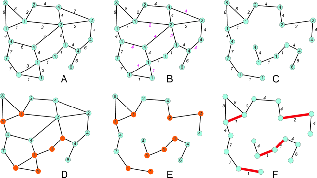
Figure 4: A: Given an edge weighted graph, the node weights are obtained by the erosioin $\varepsilon_{ne}e.$
B: A subsequent dilation $\delta_{en}$ produces the opening $\gamma_{e}e=\delta_{en}\varepsilon_{ne}e.\$The edges which are not invariant by the opening are in red.
C: The edges which are not invariant by the opening $\gamma_{e}$ are the edges which are not the lowest adjacent edge of one of their extremities. The suppression of all these edges produces the flooding graph.
D: The regional minima of the complete node weighted graph do not correspond to the regional minima of the edge weighted graph depicted in F.
E: The regional minima of node weighted flooding graph do correspond to the regional minima of the edge weighted graph depicted in F.
F: The regional minima of the edge weighted flooding graph.

4.4.3 Transforming a node weighted graph into a flooding graph

Consider an arbitrary node weighted graph $G_{n}$with node weights $n,$ and without edge weights. The operator $\circlearrowright G$ adds a loop edge between each isolated regional minimum and itself, producing a graph invariant by $\varphi_{n}.\$The nodes verify $n=\varepsilon_{ne}\delta_{en}n.$

If we assign to the edges of $G_{n}$ weights equal to $e=\delta_{en}n,$ then $n=\varepsilon_{ne}\delta_{en}n=\varepsilon_{ne}e$ and the resulting graph is a flooding graph.

Illustration

Fig.5A presents a node weighted graph. It is not invariant by $\varphi_{n}$ as it has isolated regional minima. One adds a loop edge linking each isolated regional minimum with itself, producing the graph in fig.5B. The dilation $\delta_{en}$ produces the edge weights. The resulting edge and node weighted graph in 5C is a flooding graph. The regional minima have been highlighted by distinct colors. Again, the identity between flooding paths and flooding chains is clearly visible.

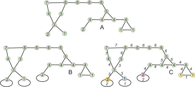
Figure 5: A: A node weighted graph.
B: A loop edge is added, linking each isolated regional minimum with itself.
C: The edge weights are produced by the dilation $\delta_{en}.\$The resulting graph is a flooding graph. 

4.5 Temporary conclusion

We have presented how to derive from any node or edge weighted graph a flooding graph with the same regional minima. To each flooding path corresponds a flooding chain with the same weight distribution, as each node is followed by an edge with the same weight. The reverse also is true: to each flooding chain corresonds a flooding path with the same weight distribution.

The catchment basins, as defined earlier, are exactly the same. As all non ascending paths and chains are accepted for defining the catchment basins, we also have the largest overlaping zones between them.

Two classes of watershed algorithms have been developed, the ones for node weighted graphs, the others for edge weighted graphs. Since we have a one to one correspondance between flooding paths and flooding chains, each algorithm developed for a node (resp. edge) weighted graph may now also be applied for an edge (.resp node) weighted graph, by applying it on the associated flooding graph.

5 Reducing the number of catchment basins and the size of their overlapping zones

5.1 Estimating the number of catchment basins

Fig.6A1 presents a flooding graph with three regional minima. The three associated catchment basins overlap at a node p with weight 4. In order to break the tie, only one edge adjacent to the node $p$ should be kept, and the others suppressed. Three solutions are possible, illustrated by the figures 6A2, B2 and C2. There is no means to decide between one or the other solution if one considers only the weight on one edge. If one considers the first two edges of each flooding path, we obtain a lexicographic measure, by concatenating the weight of the first and the second, illustrated in fig. 6B1. There remains now two choices between the edges with weights $43,$ represented in figures figures 6B2 and C2. Considering a third edge along the flooding paths leaves only one choice, as the edge with the weight $431$ is the lowest. The corresponding waterhed segmentation is presented in fig. 6C2. This example shows that we are able to reduce the number of partitions associated to a flooding graph, if one considers not only the first neighboring nodes or edges in the flooding paths or chains, but a number of nodes, ordered in a lexicographic order.

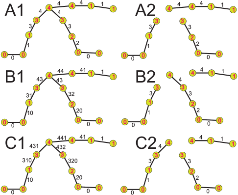
Figure 6: A1 : To each edge is assigned its lexicographic distance of depth $1$ to the nearest regional minimum. A node with weight $4$ has three adjacent edges with weight $4.\$Keeping only one of them and suppressing the others yields 3 possible partitions represented in A2, B2 and C2.
B1: To each edge is assigned its lexicographic distance of depth $2$ to the nearest regional minimum. The node with weight $4$ has now two lowest adjacent edges with a weight $43.\$Keeping only one of them and suppressing the other adjacent edges yields 2 possible partitions represented in B2 and C2.
C1: To each edge is assigned its lexicographic distance of depth $3$ to the nearest regional minimum. The node with weight $4$ has only one lowest adjacent edges with a weight $431.\$Keeping only this one of them and suppressing the other adjacent edges yields 1 possible partitions represented in C2.

By defining a lexicographic order among the flooding chains of depth $3$ has permitted to break the ties, leaving only one solution.

5.2 A lexicographic order relation between downwards paths

Given a node or weighted graph we first derive its flooding graph $G=[E,N].$ We associate to $G$ an oriented graph $\overrightarrow{G}$ by replacing the edge $(p,q)$ by an arrow $\overrightarrow{pq}$ if $n_{p}\geq n_{q}\$and  by two arrows $\overrightarrow{pq}$ and $\overrightarrow{qp}$ if $n_{p}=n_{q}$. The loop edge linking an isolated regional minimum node $m$ with itself also is replaced by an arrow $\overrightarrow{mm}.$ The graph $\overrightarrow{G}$ verifies the property $(P)$: $\forall p\in N,$ there exists at least an oriented path $\overrightarrow{\pi}$ of $\overrightarrow{G}$ (with a positive or null length) linking $p$ with a regional minimum. We define the catchment basin of a regional minimum as the set of nodes linked by an oriented path with this minimum. Obviously, each node belongs to at least one catchment basins. Catchment basins may overlap and form a watershed zone when two paths having the same node as origin reach two distinct regional minima. We aim at pruning the graph $\overrightarrow{G},$ without any arbitrary choices, and get a partial graph $\overrightarrow{G^{\prime}}$ for which the property $(P)$ still holds but the watershed zones are smaller.

As soon the path $\overrightarrow{\pi}$ reaches a regional minimum, it may be prolonged into a path of infinite length, by infinitely cycling between $2$ nodes within the regional minimum or along the loop joining each isolated regional minimum with itself. All oriented paths or chains are thus of infinite length. And we may consider them, either in their full infinite length or consider only the first $k$ edges.

We now define a family of preorder relations (order relation without antisymmetry) between the paths of $\overrightarrow{G}.$

The lexicographic preorder relation of length $k$ compares the infinite paths $\pi=(p_{1},p_{2},...p_{k},...)$ and $\chi=(q_{1},q_{2},...q_{k},...)$ by considering the $k$ first nodes and edges:
* $\pi\prec^{k}\chi$ if $n_{p_{1}}<n_{q1}$ or there exists $t<k$ such that $\forall l<t:n_{p_{l}}=n_{q_{l}}$ $n_{p_{t}}<n_{q_{t}}$
* $\pi\preceq^{k}\chi$ if $\pi\prec^{k}\chi$ or if $\forall l\leq k:n_{p_{l}}=n_{q_{l}}.$

This preorder relation is total, as it permits to compare all paths ; for this reason, among all paths linking a node $p$ with a regional minimum, there exists always at least one which is the smallest for $\preceq^{k}.$ We say that this path is the steepest for the lexicographic order of depth $k.$

For $k=\infty,$ we consider the infinite paths and we simply write $\preceq$.

If $\pi$ and$\chi$ are two paths of infinite length verifying $\pi\preceq\chi$ , then the paths $\pi_{l}$ and$\chi_{l}$ obtained by skipping the $l$ first nodes also verify $\pi_{l}\preceq\chi_{l}.\$If $\pi$ is the smallest path linking its origin with a regional minimum, then $\pi_{l}$ is the smallest path leading from $p_{l+1}$ to the same regional minimum.

5.2.1 Nested catchment basins

Consider two lexicographic order relations $\prec^{k}$ and $\prec^{l}$ with $l>k,$ then for $\pi_{1}$ and $\pi_{2}:$ $\pi_{1}\prec^{k}\pi_{2}\Rightarrow\pi_{1}\prec^{l}\pi_{2}$ or equivalently $\pi_{1}\succeq^{l}\pi_{2}\Rightarrow\pi_{1}\succeq^{k}\pi_{2}:$ the steepest path for the lexicographic order $l$ also is steepest for the lexicographic order $k$. As a consequence, a catchment basin for $\succeq^{l}$ is included in the catchment basin for $\succeq^{k}.$

For increasing values of $k,$ the catchment basins become larger, are nested, and the watershed zones are reduced or vanish. For $k=\infty,$ a node is linked by two minimal paths with two distinct minima, only if these two paths have exactly the same weights, which seldom happens in natural images. In particular, if the regional minima have distinct weights, the catchment basins form a partition.

5.2.2 Pruning the flooding graph to get steeper paths

We associate to each order relation $\preceq^{k}$ of length $k$ a pruning operator $\downarrow^{k}.\$The pruning $\downarrow^{k}$ suppresses each edge which is not the first edge of a steepest path for $\preceq^{k}$ among all paths with the same origin .After pruning, each node outside the regional minima is the origin of one or several $k-$steepest flooding tracks or $k-$steepest flooding paths We say that the graph $\downarrow^{k}G$ has a k-steepness or is k-steep. As for $l>k,$ $\pi_{1}\succeq^{l}\pi_{2}\Rightarrow\pi_{1}\succeq^{k}\pi_{2}$, we have $\downarrow^{l}G\subset\downarrow^{k}G$. Furthermore $\downarrow^{k}\downarrow^{l}G=\downarrow^{l}\downarrow^{k}G=\downarrow^{k\vee l}G.$

Remark 2

Each pruning $\downarrow^{k}G$ suppresses a number of edges still present in $\downarrow^{k-1}G$ ; it suppresses them all, without doing any arbitrary choices between them.

Particular k-steep graphs

Applied to an arbitrary graph, the pruning $\downarrow^{1}=\ \downarrow$ suppresses the edges which are not the lowest edge of one of their extremities. In a flooding graph, each edge it the lowest edge of one of its extremities and $\downarrow^{1}$ is inoperant. The pruning $\downarrow^{2}$ keeps for each node $i$ the adjacent edges linking $i$ with one of its lowest neighboring nodes. The pruning $\downarrow^{\infty}$ only keeps the first edge of the steepest paths.

Lemma: Any oriented path in $\downarrow^{k}G$ of length $k$ is of maximal steepness for $\preceq^{k}.$

For this reason, a node $p$ belongs to a $k-$catchment basin associated to a node $m$ in a regional minimum, if there exists an oriented path in $\downarrow^{k}G$ from $p$ to $m.$For increasing values of $k,$ the catchment basins are decreasing, and so are the overlapping zones between them.

5.3 Erosions, dilations and openings on oriented graphs

The operator $\downarrow^{k}$ defined above has nice properties but is not a local operator. It is however possible to implement it using only local operators as we present now.

5.3.1 Two adjunctions on oriented graphs

The adjunctions $(\delta_{en},\varepsilon_{ne})$ and $(\delta_{ne},\varepsilon_{en})$ were defined for non oriented graphs. We now define the equivalent operators for oriented graphs.

The erosion from arrows to nodes assigns to each node $p$ the minimal weight of all arrows having $p$ as origin: $\left(\overrightarrow{\varepsilon}_{ne}\right)_{p}={\textstyle\bigwedge\limits_{q\mid p\rightarrow q}}e_{\overrightarrow{pq}}.$

The dilation is obtained by adjunction. Consider a weight distribution $s$ on the nodes of the oriented graph and a weight distribution $e$ on the arrows.

${\textstyle\bigwedge\limits_{q\mid p\rightarrow q}}e_{\overrightarrow{pq}}\geq s_{p}\Leftrightarrow\$for $q\mid p\rightarrow q:e_{\overrightarrow{pq}}\geq s_{p}\Leftrightarrow e_{\overrightarrow{pq}}\geq{\textstyle\bigvee\limits_{q\mid p\rightarrow q}}s_{p}=s_{p}=\left(\overrightarrow{\delta}_{en}s\right)_{\overrightarrow{pq}}$

The dilation $\left(\overrightarrow{\delta}_{en}s\right)_{\overrightarrow{pq}}$ assigns to the arrow $\overrightarrow{pq}$ the weight of its origin $p.$

We also will need the dual erosion $\left(\overrightarrow{\varepsilon}_{en}n\right)_{\overrightarrow{pq}}$ assigning to the arrow $\overrightarrow{pq}$ the weight of its extremity $q$.

5.3.2 The invariants by the opening

Consider an arrow $\overrightarrow{pq}.\ \$The erosion $\overrightarrow{\varepsilon}_{ne}$ assigns to the node $p$ the minimal weight of all arrows having $p$ as origin. The subsequent dilation assigns to the arrow $\overrightarrow{pq}$ the weight of $p,$ i.e. the the minimal weight of all arrows having $p$ as origin. Thus if $\left(\overrightarrow{\gamma}_{e}e\right)_{\overrightarrow{pq}}$ leaves the arrow $\overrightarrow{pq}$ unchanged, it means that this arrow is one of the lowest arrows having $p$ as origin.

We define a pruning operator $\downharpoonright\overrightarrow{G}$ which cuts all arrows which are not invariant by the opening $\overrightarrow{\gamma}_{e},$ i.e. which are not one of the lowest edges of their origin.

5.3.3 The oriented flooding graphs

We say that an edge and node weighted graph is an oriented flooding graph if the weights of the nodes and of the arrows verify:

for the node weights $n_{p}=\left(\overrightarrow{\varepsilon}_{ne}\right)_{p}$ and for the edge weights: $e_{\overrightarrow{pq}}=\left(\overrightarrow{\delta}_{en}n\right)_{\overrightarrow{pq}}.$ Such a graph is invariant by the opening $\overrightarrow{\delta}_{en}\overrightarrow{\varepsilon}_{ne}=\overrightarrow{\gamma}_{e}$ and by the closing $\overrightarrow{\varepsilon}_{ne}\overrightarrow{\delta}_{en}=\overrightarrow{\varphi}_{n}.$

5.4 Pruning a flooding graph with local operators and without arbitrary choices. 

5.4.1 The pruning operator

We start with a node and edge weighted flooding graph $G.\$As explained above, we associate to $G$ an oriented graph $\overrightarrow{G}$ by replacing the edge $(p,q)$ by an arrow $\overrightarrow{pq}$ if $n_{p}\geq n_{q}\$and  by two arrows $\overrightarrow{pq}$ and $\overrightarrow{qp}$ if $n_{p}=n_{q}$. The loop edge linking an isolated regional minimum node $m$ with itself also is replaced by an arrow $\overrightarrow{mm}.$

It is easy to show that if $G$ is a flooding graph, then $\overrightarrow{G}$ is an oriented flooding graph.

In order to identify edges which belong to flooding chains of maximal lexicographic $k-$steepness, we have to shift the weight distribution of nodes and weights along the oriented flooding track upwards. This is obtained thanks to the erosion $\left(\overrightarrow{\varepsilon}_{en}n\right)_{\overrightarrow{pq}}$ which assigns to the arrow $\overrightarrow{pq}$ the weight of its extremity $q.$

After this erosion, we get an edge weight distribution which is not invariant anymore by the opening $\overrightarrow{\gamma}_{e}.\$Applying the pruning operator $\downharpoonright\overrightarrow{G}$ leaves a graph which is invariant by $\overrightarrow{\gamma}_{e}.\$A final erosion $\left(\overrightarrow{\varepsilon}_{ne}\right)_{p}$ assigns to the nodes their new weights.

Thus we have applied to $\overrightarrow{G}$ the following operators :$\overrightarrow{\varepsilon}_{en}$ from nodes to arrows, the pruning operator $\downharpoonright$ on the edges followed by a last erosion $\overrightarrow{\varepsilon}_{ne}$ from the edges to the nodes, producing node weights $n=\overrightarrow{\varepsilon}_{ne}e.\$The resulting graph is an oriented flooding graph. Indeed the edges verify $e=\overrightarrow{\gamma}_{e}e=\overrightarrow{\delta}_{en}\overrightarrow{\varepsilon}_{ne}e=\overrightarrow{\delta}_{en}n.\$We call $\zeta$ the succession of these three operators. In every day words, the operator $\zeta$ does the following: each node is assigned the minimal weight of all arrows for which it is origin ; each arrow is assigned a weight equal to its extremity ; each arrow with a higher weight than its origin is suppressed.

Every time that we apply $\zeta,$ new edges are pruned and the weight distribution along the flooding paths and chains moves upwards. For $\zeta^{(k)}$ we obtain a graph $\zeta^{(k)}\overrightarrow{G}$ which contains only flooding paths and chains of steepness $\geq k+1.$

5.4.2 Illustration

Case of an initially edge weighted graph

The fig. 7A represents an edge weighted graph on which the regional minima edges are indicated in red. Fig. 7B presents the associated flooding graph $G$. We associate to $G$ an oriented graph $\overrightarrow{G}$ by replacing the edge $(p,q)$ by an arrow $\overrightarrow{pq}$ if $n_{p}\geq n_{q}\$and  by two arrows $\overrightarrow{pq}$ and $\overrightarrow{qp}$ if $n_{p}=n_{q}$ and get fig. 7C. The operator $\zeta$ produces a new weight distribution for both nodes and edges in fig. 7D. Furthermore two arrows are cut as they are not invariant by the opening $\overrightarrow{\gamma}_{e}.$ As each connected component contains only one regional minimum, we can stop the pruning and we obtain the final watershed partition. This partition is indicated in false color on top of the flooding graph $G$ in fig.7E and also in false color on top of the complete initial graph in fig.7F.

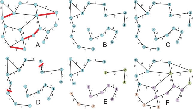
Figure 7: A: An edge weighted graph. The edges in red are the regional minima edges.
B: The associated flooding graph $G$
C: The oriented flooding graph
D: Applying the operator $\zeta$ to the oriented flooding graph suppresses two edges, and leaves 4 connected components, containing each a regional minimum.
E: The resulting partition superimposed on the flooding graph.
F: The resulting partition superimposed on the initial edge weighted graph

Case of an initially node weighted graph

Fig.8A presents a node weighted graph. It contains a number of some difficulties, like the presence of 2 plateaux and of a buttonhole at the node with weight $3.$ In a first step we add loop edges linking each isolated regional minimum with itself as shown in fig.8B. The next step produces edge weights by the dilation $\delta_{en}$ of the node weights, yielding the initial flooding graph $G$ in fig.8C The oriented graph $\overrightarrow{G}$ is produced in fig.8D. With each new applications of the operator $\zeta$ the graph $\overrightarrow{G}$ is further pruned, yielding the graphs of fig.8 E,F and G. Fig.8H transports the arrows of the graph fig.8G onto the graph $\overrightarrow{G}.\$The remaining flooding tracks are clearly visible, on a graph which has kept the initial node weights.

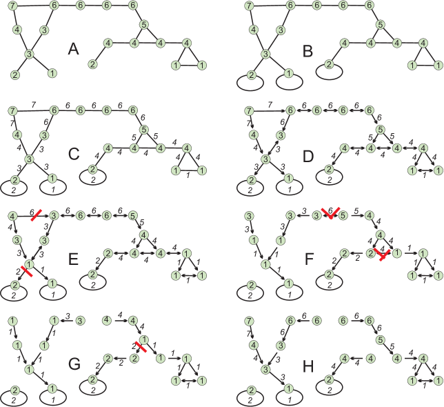
Figure 8: A: A node weighted graph. 
B: A loop edge is added linking each isolated regional minimum with itself
C: The dilation $\delta_{en}$ assigns weights to the edges and produces the flooding graph $G$
C: The flooding graph is transformed into an oriented flooding graph
E,F,G: Applying three times the operator $\zeta$ to the oriented flooding graph.    Each new application suppresses new edges, finally leaving flooding paths and chains with a lexicographic steepness of $4.\$It leaves 4 connected components, containing each a regional minimum.
E,F,G: The resulting partition superimposed on the flooding graph
F: The resulting partition superimposed with the oriented flooding graph

6 Introducing arbitrary choices when needed

6.1 Arbitrary choices on the flooding graph

We now summarize the results of this study. Starting from a node or edge weighted graph, we want to construct a watershed partition, without arbitrary choices, or with a minimum number of arbitrary choices. In a first step we derive the flooding graph. An edge weighted graph looses the edges which are not the lowest neighboring edges of one of their extremities, but keeps the edge weights. The node weights are obtained by the erosion $\varepsilon_{ne}.\$To a node weighted graph are added some loops linking each isolated regional minimum with itself. The node weights keep their initial weights and the edge weights are obtained by the dilation $\delta_{en}.$ In both cases we obtain a graph with a perfect coupling between edge and node weights ; furthermore, the edge regional minima span the node regional minima. And the flooding chains span the flooding paths, each node being followed by an edge with the same weight.

Method 1: The ties are broken by a watershed algorithm applied on the flooding graph. Any algorithm of the literature developed for node (resp. edge) weighted graphs may now be applied to the flooding graph, even if the initial graph is an edge (resp. node) weighted graph. The algorithm of B.Marcotegui et al [8] for constructing the watershed on an edge weighted graph is derived from Prim’s algorithm for constructing a minimum spanning tree or forest. This algorithm is myopic and considers only flooding chains with a lexicographic depth equal to 1. The algorithms proposed in [5] are or the same myopic type. Using an algorithm [9] based on the topographic distance [10],[11], and applied to node weighted graphs, choses flooding chains with a lexicographic depth equal to 2, and for this reason are more selective. Such an algorithm, designed for node weighted graphs may now be applied to a graph which initially was edge weighted. The arbitrary choices for producing a watershed partition is taken in charge by the watershed algorithms applied to the flooding graph. In the case of [9] or [8], by the scheduling of the shortest distance algorithm (ultrametric flooding distance for node weighted graphs or topographic distance for node weighted graphs). These are only a few examples of algorithms which may be used, among a large number of others.

6.2 Arbitrary choices after choiceless prunings of the flooding graph

We have seen how to reduce the number of flooding tracks and paths. The flooding graph $G$ is transformed into an oriented graph $\overrightarrow{G}.\$The operator $\zeta$ prunes further this graph, again without arbitrary choices. After $k$ iterations, only the flooding paths or flooding tracks of the graph $G$ with a lexicographic depth $k+1$ remain. We then "transport" the arrows of the graph $\zeta^{(k)}\overrightarrow{G}$ onto the flooding graph $G$ and get a graph $G^{(k)}:$ we keep an edge $(p,q)$ of $G$ if and only if there exists an arrow $\overrightarrow{pq}$ or $\overrightarrow{qp}$ in the graph $\zeta^{(k)}\overrightarrow{G}.\$Like that we obtain a flooding graph $G$ in which the only remaining flooding tracks and paths have a steepness $\geq k+1.$ A node $p$ belongs to two catchment basins, if there exists two flooding paths towards the corresponding minima, with identical $k+1$ first edges forming a track of $k+1$ maximal steepness. Fig.9 presents 4 pruning states of the node weighted graph in fig.8A. Fig.9A presents the associated flooding graph (without the loops on the isolated regional minima), where the edge weights have been added. Two types of methods may be applied to this graph.

Method 2: After $k$ steps of pruning, the graph $G^{(k)}$ has only flooding paths and chains of steepness $\geq k+1.\$Again any algorithm developed for node or edge weighted graph may be applied to this graph. But as the remaining flooding paths are extremely scarce, even the loosest and most myopic algorithms will do a good job. In particular the algorithm by B.Marcotegui which normally selects flooding paths of steepness $\geq 1$ now selects paths of steepness $\geq k+1,$ as they are the only available. The same is true for the algorithm based on the topographic distance, selecting flooding paths of steepness $\geq 2.$ The remaining arbitrary choice, if any, is taken in charge by the scheduling of the shortest distance algorithm (ultrametric flooding distance for node weighted graphs or topographic distance for node weighted graphs).

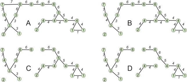
Figure 9: Four graphs with flooding paths of increasing steepness and decreasing overlapping zones of the catchment basins.

Method 3: We continue the pruning $\zeta^{(k)}\overrightarrow{G}$ until there remain no arrows which are head to tail, except in the regional minima. This is the case in fig.8F. There exists a node with weight $4$ which is the origin of two arrows with weight $4.\$If we arbitrarily suppress one of them, we are also done and have a partition. There are two solutions possible at this stage of pruning. Thus if a node is the origin of several arrows, one leaves only one. (this method has often been used in hardware implementations, but without preliminary pruning [3],[7]).

6.3 Maximal prunings with scarcely needed choices

For $k=\infty,$ we obtain a maximal pruning of the flooding graph. In fact we may stop as soon the graph is cut into a number of components containing each one regional minimum. The node and edge weights remain identical as in the graph $G,$ but there remains only a minimal number of flooding paths and chains. A node will be linked to two distinct minima by two flooding chains only if there exists two paths with exactly the same weight distributions towards these two minima ; this will rarely happen in natural images. If the minima have distinct weights, each node is linked with one and only one minimum by a flooding path of maximal steepness.

Method 4: We continue the pruning $\zeta^{(k)}\overrightarrow{G}$ until each connected component contains only one regional minimum and we are done. If this cannot be achieved, then we resort to method 3. After an infinite number of prunings, $\zeta^{(\infty)}\overrightarrow{G}$ does not contain any head and tail arrows and method 3 can be applied.

Method 5: We slightly change the weights of the minima so that they are all distinct. We continue the pruning $\zeta^{(k)}\overrightarrow{G}$ until each connected component contains only one regional minimum and we are done. We know that this will happen for $k<\infty.$

7 Conclusion

We have established that node and weighted graphs represent the same topography, with the same minima and the same catchment basins. We have presented a method to reduce the overlapping zones of the catchment basins without arbitrary choices. We finally have presented how to introduce such arbitrary choices if needed.

References

- [1] C. Berge. Graphs. Amsterdam: North Holland, 1985.
- [2] S. Beucher and C. Lantuéjoul. Use of watersheds in contour detection. In Proc. Int. Workshop Image Processing, Real-Time Edge and Motion Detection/Estimation, 1979.
- [3] Moga A. Bieniek, A. An efficient watershed algorithm based on connected components. Pattern Recognition, 33(6):907–916, 2000. cited By (since 1996) 78.
- [4] S. Beucher. Watershed, hierarchical segmentation and waterfall algorithm. ISMM94 : Mathematical Morphology and its applications to Signal Processing, pages 69–76, 1994.
- [5] Jean Cousty, Gilles Bertrand, Laurent Najman, and Michel Couprie. Watershed cuts: Minimum spanning forests and the drop of water principle. IEEE Transactions on Pattern Analysis and Machine Intelligence, 31:1362–1374, 2009.
- [6] M. Gondran and M. Minoux. Graphes et Algorithmes. Eyrolles, 1995.
- [7] F. Lemonnier. Architecture Electronique Dédiée aux Algorithmes Rapides de Segmentation Basés sur la Morphologie Mathématique. PhD thesis, E.N.S. des Mines de Paris, 1996.
- [8] B. Marcotegui and S. Beucher. Fast implementation of waterfalls based on graphs. ISMM05 : Mathematical Morphology and its applications to Signal Processing, pages 177–186, 2005.
- [9] F. Meyer. Un algorithme optimal de ligne de partage des eaux. In Proceedings Congrès AFCET, Lyon-Villeurbanne, pages 847–857, 1991.
- [10] F. Meyer. Topographic distance and watershed lines. Signal Processing, pages 113–125, 1994.
- [11] Laurent Najman and Michel Schmitt. Watershed of a continuous function. Signal Processing, 38(1):99 – 112, 1994. Mathematical Morphology and its Applications to Signal Processing.
- [12] L. Najman and h. Talbot (ed) Mathematical morphology Wiley editor, 2012
- [13] Jos B. T. M. Roerdink and Arnold Meijster. The watershed transform: Definitions, algorithms and parallelization strategies. Fundamenta Informaticae, 41:187–228, 2001.