On the minimum FLOPs problem in the sparse Cholesky factorization

Abstract

Prior to computing the Cholesky factorization of a sparse symmetric positive definite matrix, a reordering of the rows and columns is computed so as to reduce both the number of fill elements in Cholesky factor and the number of arithmetic operations (FLOPs) in the numerical factorization. These two metrics are clearly somehow related and yet it is suspected that these two problems are different. However, no rigorous theoretical treatment of the relation of these two problems seems to have been given yet. In this paper we show by means of an explicit, scalable construction that the two problems are different in a very strict sense: no ordering is optimal for both fill and FLOPs in the constructed graph.

Further, it is commonly believed that minimizing the number of FLOPs is no easier than minimizing the fill (in the complexity sense), but so far no proof appears to be known. We give a reduction chain that shows the NP hardness of minimizing the number of arithmetic operations in the Cholesky factorization.

siam sparse Cholesky factorization, minimum fill, minimum operation count, computational complexity

siam 65F50, 65F05, 68Q17

1 Introduction

Let $A\in\mathbb{R}^{n\times n}$ be a sparse, real, symmetric positive definite (SPD) matrix and consider the Cholesky factorization of $A$ with symmetric pivoting, that is, $PAP^{T}=LL^{T}$, where $L$ is a lower triangular matrix and $P$ is a permutation matrix. Assuming no accidental cancellation, the nonzero pattern of $L+L^{T}$ depends solely on the choice of $P$ and contains the nonzero pattern of $PAP^{T}$. Nonzero elements of $L$ at positions that are structural zeros in $PAP^{T}$ are called fill elements. Determining a permutation matrix $P$, such that the number of these fill elements is minimum, is an NP hard problem [24]. Since the arithmetic work in terms of floating point operations for the computation of the Cholesky factor $L$ is solely determined by the permutation matrix $P$ as well, one may wonder how the number of fill elements and arithmetic work are related. In this paper we study this relationship and give an NP hardness result for the minimization of the arithmetic work.

Gaussian elimination for symmetric matrices is very conveniently described in terms of undirected graphs. For example, the Cholesky factorization of $A$ can be seen as an embedding of the graph $G(A)$ of $A$ into a triangulated supergraph $G^{+}$ of $G$. In this work we assume familiarity with some basic graph theoretic terminology and concepts such as the elimination game, chordality and perfect elimination orderings (PEOs). Useful references that cover all the terminology we use are [22] and [13].

Let $G=(V,E)$ be a simple undirected graph with $n$ vertices. If $F\subseteq V\times V\setminus E$ is a set of fill edges such that $G^{+}=(V,E\cup F)$ is chordal, then there exists a PEO $\alpha:V\rightarrow\{1,\dotsc,n\}$ for $G^{+}$. When carrying out vertex elimination on $G^{+}$ according to $\alpha$, denote by $\mbox{d}(\alpha^{-1}(i))$ the degree of the $i$-th vertex in the course of the elimination process (the elimination degree of $\alpha^{-1}(i))$. Minimizing the quantity

$$\mbox{nnz}(\alpha)=\sum_{i=1}^{n}(\mbox{d}(\alpha^{-1}(i))+1)$$

over all triangulations $G^{+}=(V,E\cup F)$ is what we call the MinimumFill problem in this work (equivalently, one could minimize $|{F}|$). If $G$ is the graph of a sparse symmetric positive definite matrix $A$, then $\mbox{nnz}(\alpha)$ is the number of nonzero elements in the Cholesky factor of $A$ when carrying out the factorization in the ordering $\alpha$.

Another metric of interest is the number of floating point operations (FLOPs) that are required for the computation of the Cholesky factor in the given ordering $\alpha$. If we account for all additive, multiplicative and square-root operations for the computation of the Cholesky factor, the total number of such FLOPs is given by

$$\text{flop}(\alpha)=\sum_{i=1}^{n}(\mbox{d}(\alpha^{-1}(i))+1)^{2}.$$

Minimizing $\text{flop}(\alpha)$ over all triangulations of $G$ is the MinimumFLOPs problem.

It is important to note that the multiset of elimination degrees $\{\mbox{d}(\alpha^{-1}(i))\}_{i=1}^{n}$ is the same for all PEOs $\alpha$ of a triangulation [22, Thm. 4]. Hence, the quantities $\mbox{nnz}(\cdot)$ and $\text{flop}(\cdot)$ depend only on the triangulation $G^{+}$ (see also [8]).

The MinimumFLOPs problem has received much less attention in the literature than the MinimumFill problem. It is also occasionally noted that the two metrics are related (e.g. [11, §7], [21, ch. 59]) and it is occasionally noted that the two problems are believed to be different (e.g. [22, sec. 4.1.2]). However, a rigorous investigation of the relation of these two problems seems to be missing in the literature.

In section 2 we discuss a class of graphs, parameterized by the number of vertices, for which all optimal orderings with respect to either one metric are strictly suboptimal for the other. A third ordering problem to which we relate these findings is the Treewidth problem. In the context of multifrontal methods [7, 17], this problem asks for an elimination ordering such that the largest front size is minimum [5]. It is also a parameter in the lower bound for the amount of communication in the parallel sparse Cholesky factorization, since it determines the size of a largest dense submatrix that has to be factorized. Finally, we briefly discuss ordering heuristics from the viewpoint of the minimum FLOPs problem.

In section 3 we give a formal NP hardness result for MinimumFLOPs. While it is well known that minimizing the fill is NP hard [24] and one expects that minimizing the number of arithmetic operations is no less difficult, it seems that such a proof has not been given before.

1.1 Notation

We use the following notation throughout this paper. The Cartesian product of two sets $P$ and $Q$ is denoted by $P\times Q$. For two graphs $G_{1}=(V_{1},E_{1})$ and $G_{2}=(V_{2},E_{2})$ we define their sum $G_{1}+G_{2}\mathrel{\mathop{:}}=(V_{1}\cup V_{2},E_{1}\cup E_{2})$ and their join $G_{1}\vee G_{2}\mathrel{\mathop{:}}=(V_{1}\cup V_{2},E_{1}\cup E_{2}\cup(V_{1}\times V_{2}))$. By $K_{s}$ we refer to the complete graph (or clique) on $s$ vertices. For a graph $G=(V,E)$ and a vertex $v\in V$, we denote by $\mathcal{N}_{G}\left(v\right)\subseteq V$ the neighborhood of $v$ in $G$, that is, the vertices adjacent to $v$. The closed neighborhood of $v$ is $\mathcal{N}_{G}\left[v\right]\mathrel{\mathop{:}}=\mathcal{N}_{G}\left(v\right)\cup\{v\}$. Denote the vertex degree and the closed vertex degree of $v$ by $\mbox{d}_{G}(v)=|{\mathcal{N}_{G}\left(v\right)}|$ and $\mbox{d}_{G}[v]=|{\mathcal{N}_{G}\left[v\right]}|$, respectively. We omit the reference to the graph $G$ in the notation whenever the context permits. For example, in the context of vertex elimination, $\mbox{d}[\alpha^{-1}(i)]$ always refers to the $i$-th elimination degree. Sometimes we explicitly refer to the vertex and edge sets of a graph $G$ by $V(G)$ and $E(G)$. Using this notation we formally restate the two problems of interest as decision problems (recall that $\mbox{d}(\alpha^{-1}(i))$ refers to the elimination degree and notice that $\mbox{d}(\alpha^{-1}(i))+1=\mbox{d}[\alpha^{-1}(i)]$).

MinimumFill
Instance: Graph $G=(V,E),n=|{V}|,k\in\mathbb{N}$ Question: Is there a set of edges $F\subseteq V\times V$ such that $(V,E\cup F)$ has a PEO $\alpha:V\rightarrow\{1,\dotsc,n\}$ with $\sum_{i=1}^{n}\mbox{d}[\alpha^{-1}(i)]\leq k$?

MinimumFLOPs
Instance: Graph $G=(V,E),n=|{V}|,k\in\mathbb{N}$ Question: Is there a set of edges $F\subseteq V\times V$ such that $(V,E\cup F)$ has a PEO $\alpha:V\rightarrow\{1,\dotsc,n\}$ with $\sum_{i=1}^{n}\mbox{d}[\alpha^{-1}(i)]^{2}\leq k$?

2 Minimum fill and minimum FLOPs are different

In this section we present a class of graphs for which minimizing fill and minimizing FLOPs are different problems. Interestingly, a structurally similar class of graphs is used in [15, p. 14] to show that MinimumFill and Treewidth are different. The treewidth problem is yet another NP hard problem [4] that can be formulated using elimination degrees:

Treewidth
Instance: Graph $G=(V,E),n=|{V}|,k\in\mathbb{N}$ Question: Is there a set of edges $F\subseteq V\times V$ such that $(V,E\cup F)$ has a PEO $\alpha:V\rightarrow\{1,\dotsc,n\}$ with $\max_{i}\mbox{d}[\alpha^{-1}(i)]\leq k$?

We will use the abbreviation $\omega(\alpha)\mathrel{\mathop{:}}=\max_{i}\mbox{d}[\alpha^{-1}(i)]$, which is exactly the clique number of the triangulation of $G$ corresponding to $\alpha$.

We will show that MinimumFill, MinimumFLOPs and Treewidth are different problems in a very strict sense. In section 2.1 we explore all minimal triangulations of a parameterized class of graphs (again, see [13] for an overview of the terminology). Using specific values for the parameters in section 2.2, we show that minima for the three optimization problems are attained at distinct triangulations. Finally, in section 2.3 we discuss the minimum FLOPs problem from the viewpoint of ordering heuristics.

2.1 An instructive class of graphs

In this section we study a class of graphs whose set of minimal triangulations is sufficiently simple to analyse and yet general enough to show that the extrema of minimum fill and minimum FLOPs are attained at different triangulations. In [15, p. 14] it is pointed out that MinimumFill and Treewidth are different problems using graphs from this class. In that monograph the author refers to an unpublished report for the details. Our study covers this aspect as well.

A useful reference for all facts and results on minimal triangulations which we assume here is the survey by Heggernes [13]. We recall that every inclusion minimal triangulation can be obtained through vertex elimination along some elimination ordering. Such orderings are called minimal elimination orderings (MEOs).

Figure 1: The graph $G(l,t,c)$

The graph we want to study consists of a cycle $C_{l}$ on $l$ vertices, a clique $K_{c}$ on $c$ vertices and an independent set $S_{t}$ of $t$ vertices, plus all possible edges between the cycle and the other $t+c$ vertices (see Fig. 1). More formally, for numbers $4\leq l,t,c\in\mathbb{N}$ the graph is defined as $G=C_{l}\vee(S_{t}+K_{c})$. First we will characterize all minimal triangulations of $G$. In fact only two types of triangulations exist; they are shown in Fig. 2.

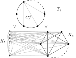
Figure 2: The two types of triangulations of $G(l,t,c)$, $T_{1}$ and $T_{2}$. Gray edges are fill edges.

Proposition 2.1.

The graph $G\mathrel{\mathop{:}}=C_{l}\vee(S_{t}+K_{c})$ has exactly two types of minimal triangulations $T_{1}\cong K_{l}\vee(S_{t}+K_{c})$ and $T_{2}\cong C_{l}^{+}\vee K_{t+c}$, where $C_{l}^{+}$ is a minimal triangulation of $C_{l}$.

It is easy to verify that $T_{1}$ and $T_{2}$ are indeed chordal graphs, since corresponding PEOs are readily constructed. Let $T$ be a minimal triangulation of $G$. Then there exists a minimal elimination ordering $\alpha:V(G)\rightarrow\{1,\dotsc,l+t+c\}$ for $G$ whose resulting filled graph is $T$. Let $v=\alpha^{-1}(1)$ be the first vertex to be eliminated and denote the graph arising from eliminating $v$ by $G_{v}^{+}$. We distinguish three cases:

1. : $v\in V(K_{c})$. Then $G^{+}_{v}\cong K_{l}\vee(S_{t}+K_{c-1})$, which is a chordal graph. Since $\alpha$ is a MEO for $G$, $\{\alpha^{-1}(2),\dotsc,\alpha^{-1}(n)\}$ is a PEO for $G^{+}_{v}$ and so $T\cong T_{1}$.

2. : $v\in V(S_{t})$. Then $G_{v}^{+}\cong K_{l}\vee(S_{t-1}+K_{c})$, which is a chordal graph. Since $\alpha$ is a MEO for $G$, $\{\alpha^{-1}(2),\dotsc,\alpha^{-1}(n)\}$ is a PEO for $G^{+}_{v}$ and so $T\cong T_{1}$.

3. : $v\in V(C_{l})$. Then $G^{+}_{v}\cong C_{l-1}\vee K_{t+c}$. In this graph the only chordless cycle of length at least four can possibly be $C_{l-1}$. So the minimal triangulations of $G^{+}_{v}$ are now given by the minimal triangulations of $C_{l-1}$, which implies that $T\cong T_{2}$.

It remains to show that $T_{1}$ and $T_{2}$ are minimal. We do so by showing that in both triangulations every fill edge is the unique chord of some four-cycle in $T_{1}$ and $T_{2}$. For $T_{1}$ consider any fill edge $f=(c_{i},c_{j})$ in $V(C_{l})\times V(C_{l})$ and $s\in V(S_{t}),v\in V(K_{c})$. Then $(s,c_{i},v,c_{j},s)$ is a four-cycle in $T_{1}$ whose unique chord is $f$. For $T_{2}$ let $f=(s,v)$ be a fill edge with $s\in V(S_{t})$, $v\in V(C_{k})$ and $c_{1}$, $c_{2}$ two non-adjacent vertices in $T_{2}$. Then $(c_{1},s,c_{2},v,c_{1})$ is a four-cycle in $T_{2}$ whose unique chord is $f$.

For both triangulations, we will now determine the elimination degree sequence of certain PEOs and count the number of nonzero elements in the corresponding Cholesky factors as well as the number of FLOPs necessary to compute them.

A PEO $\alpha_{1}$ for $T_{1}$ is given by ordering the $t$ vertices of $S_{t}$ first, followed by any ordering of the remaining complete graph of size $l+c$. For the elimination degree sequence we obtain:

$$\{\mbox{d}(\alpha_{1}^{-1}(i))\}_{i=1}^{l+t+c}=\{l\}_{j=1}^{t}\cup\{l+c-j\}_{j=1}^{l+c}.$$

Given that degree sequence, the nonzero-, FLOP count and clique number for the Cholesky factor corresponding to $T_{1}$ are given by

$$\mbox{nnz}(\alpha_{1}) =\sum_{j}(\mbox{d}(\alpha_{1}^{-1}(j))+1)=t(l+1)+\sum_{j=1}^{l+c}j$$ (1)

$$\text{flop}(\alpha_{1}) =\sum_{j}(\mbox{d}(\alpha_{1}^{-1}(j))+1)^{2}=t(l+1)^{2}+\sum_{j=1}^{l+c}j^{2}$$ (2)

$$\omega(\alpha_{1}) =\max_{i}{\mbox{d}(\alpha_{1}^{-1}(i))+1}=l+c$$ (3)

Another PEO for $T_{1}$ is obtained by ordering the vertices of $K_{c}$ first, followed by the vertices of $S_{t}$ and finally the vertices of $K_{l}$. Of course, the expressions (1)–(3) are the same for all PEOs.

A PEO $\alpha_{2}$ for the triangulation $T_{2}$ is obtained by the first $l-2$ vertices of a PEO for $C_{l}^{+}$ followed by an arbitrary ordering of the vertices of the remaining $K_{t+c+2}$. Noting that for every PEO of $C_{l}^{+}$ the elimination degree of the first $l-2$ vertices is $t+c+2$, we obtain the degree sequence

$$\{\mbox{d}(\alpha_{2}^{-1}(i))\}_{i=1}^{l+t+c}=\{t+c+2\}_{j=1}^{l-2}\cup\{t+c+2-j\}_{j=1}^{t+c+2}.$$

The resulting nonzero-, FLOP count and clique number are:

$$\mbox{nnz}(\alpha_{2}) =\sum_{j}(\mbox{d}(\alpha_{2}^{-1}(j))+1)=(l-2)(t+c+3)+\sum_{j=1}^{t+c+2}j$$ (4)

$$\text{flop}(\alpha_{2}) =\sum_{j}(\mbox{d}(\alpha_{2}^{-1}(j))+1)^{2}=(l-2)(t+c+3)^{2}+\sum_{j=1}^{t+c+2}j^{2}$$ (5)

$$\omega(\alpha_{2}) =\max_{i}{\mbox{d}(\alpha_{2}^{-1}(i))+1}=t+c+3$$ (6)

2.2 Minimizing FLOPs, fill and treewidth are different problems

Let $64<n\in\mathbb{N}$ and set $l=8n$, $t=5n$, $c=4n$ and consider the class of graphs from section 2.1 with these parameters. We will count the number of nonzeros and FLOPs for the two triangulations. Using (1)–(3) and (4)–(6) we obtain

$$\mbox{nnz}(\alpha_{1}) =112n^{2}+\mathcal{O}\left(n\right) \mbox{nnz}(\alpha_{2}) =\frac{225}{2}n^{2}+\mathcal{O}\left(n\right)$$

$$\text{flop}(\alpha_{1}) =896n^{3}+\mathcal{O}\left(n^{2}\right) \text{flop}(\alpha_{2}) =891n^{3}+\mathcal{O}\left(n^{2}\right)$$

$$\omega(\alpha_{1}) =12n \omega(\alpha_{2}) =9n+3,$$

and it is readily verified that the omitted lower order terms are dominated by the leading terms if $n>64$. So for this choice of values for $l$, $t$, $c$, we see that $\alpha_{1}$ yields the optimal triangulation for the fill, but not for the number of FLOPs or the size of the largest clique. The latter two metrics are minimized by $\alpha_{2}$, which is suboptimal for the fill.

If the values $l=2n+3,t=n,c=2n$, $n>3$, are chosen, one obtains the class of graphs from Kloks’ example [15, p.14]. In that case $\alpha_{1}$ minimizes both the fill and the number of FLOPs, but not the size of the largest clique. The minimum clique size is attained by $\alpha_{2}$, which is suboptimal for the fill and FLOPs:

$$\mbox{nnz}(\alpha_{1}) =10n^{2}+\mathcal{O}\left(n\right) \mbox{nnz}(\alpha_{2}) =\frac{21}{2}n^{2}+\mathcal{O}\left(n\right)$$

$$\text{flop}(\alpha_{1}) =\frac{76}{3}n^{3}+\mathcal{O}\left(n^{2}\right) \text{flop}(\alpha_{2}) =27n^{3}+\mathcal{O}\left(n^{2}\right)$$

$$\omega(\alpha_{1}) =4n+3 \omega(\alpha_{2}) =3n+3$$

Theorem 2.2.

The three chordal graph embedding problems MinimumFill, MinimumFLOPs and Treewidth are different in the sense that no two such metrics can be minimized simultaneously in general.

The three problems above are equivalent to minimizing the $1$-, $2$- and $\infty$-norm of the vector of elimination degrees over the set of all chordal embeddings. It would be interesting to learn whether all such $p$-norm minimization problems for, say, $p\in[1,\infty]$ are different in the sense of Thm. 2.2. We did some very preliminary but encouraging experiments for some pairs of $p$-norms, but did not pursue this question rigorously.

2.3 Minimum FLOPs and heuristics

The minimum degree (MD) heuristic and its variations (e.g. AMD [2], MMD [16]) are a popular class of ordering heuristics commonly used to reduce the number of fill elements in the Cholesky factor. These heuristics use the elimination degree of the vertices as their primary local criterion for ordering the vertices. Note that this criterion is in fact the canonical local criterion for minimizing the FLOPs and not the fill, in which context MD type heuristics are usually put.

The canonical criterion for locally minimizing the number of fill elements is the deficiency of a vertex, which accounts for the number of fill edges the elimination of the vertex would imply. It has been observed [19, 23] that using this criterion (or approximations of it) instead of the elimination degree usually results in less arithmetic (and fill). In fact, the authors of [23] regard reducing the number of FLOPs as their primary objective for their experiments with the deficiency criterion.

Reported experimental results for ordering heuristics like the ones above certainly have contributed to the common understanding that reducing the number of fill elements usually goes hand in hand with reducing the number of arithmetic operations and vice versa. While this behaviour is typically observed when ordering heuristics are benchmarked, it is worth pointing out that it may actually happen in practice that an ordering that implies less fill than another ordering actually causes significantly more FLOPs (or vice versa).

To confirm this we conducted a very simple experiment. We computed the ordering statistics for 1130 pattern symmetric matrices from the University of Florida (UF) sparse matrix collection [6] using AMD (2.3.0) [3] and METIS (4.0.3) [14]. For 91 of these matrices one heuristic produced fewer fill elements than the other while performing worse with respect to the FLOP count at the same time. For example, for the matrix “INPRO/msdoor” from the UF collection (id 1644), a structural problem, AMD produces about 2% fewer fill elements than METIS while requiring approximately 22% more arithmetic operations.

Finally we mention that several approximation algorithms for all three problems MinimumFill, MinimumFLOPs and Treewidth exist, e.g. [1, 5, 18].

3 Minimizing FLOPs is NP hard

We now show that minimizing the FLOP count in sparse Cholesky factorization is indeed an NP hard problem. To do so, we reduce the MaxCut problem to a certain class of quadratic arrangement problems in section 3.1. In section 3.2 we reduce such a quadratic arrangement problem to the minimum FLOPs problem via a quadratic variation of the bipartite chain graph completion problem.

3.1 Quadratic vertex arrangement problems

In the optimal linear arrangement problem, we are given a graph $G=(V,E)$ and are asked to arrange the vertices of $G$ at positive integer positions on the real line such that the sum of the implied edge lengths is minimum:

OptimalLinearArrangement (OLA)
Instance: Graph $G=(V,E)$ on $n$ vertices, $k\in\mathbb{N}$ Question: Is there a bijection $\alpha:V\rightarrow\{1,\dotsc,n\}$ s.t. $\sum_{(u,v)\in E}|\alpha(u)-\alpha(v)|\leq k$?

OLA is NP hard [10, GT42]. It is also known as MinimumOneSum (M1S) and minimizes the 1-norm of a vector of distances implied by the linear arrangement of the vertices of the graph. Other norms have been considered; for the 2-norm (MinimumTwoSum, M2S) and the infinity norm (Bandwidth) the corresponding arrangement problems are known to be NP hard [20, 12]. In contrast to these arrangement problems, the class of arrangement problems we discuss here cannot be expressed in terms of a $p$-norm of the distance vector.

Figure 3: Linear and quadratic arrangement of a graph. The quadratic cost function here is $f(x)=x^{2}$, so this is an instance of OQA(0). The cost of the linear arrangement is 5, while the quadratic cost is 27.

Instead of laying out the vertices of $G$ at equally spaced positions, we consider certain quadratically spaced positions (see Fig. 3). We call this the OptimalQuadraticArrangement($c$) (OQA($c$)) problem. Let

$$c=c_{2}X^{2}+c_{1}X+c_{0},\quad c_{0},c_{1},c_{2}\in\mathbb{N}$$ (7)

be a polynomial of degree at most 2 with non-negative integer coefficients. We regard $c$ as a parameter for the function

$$f:\{1,\dotsc,n\}\rightarrow\mathbb{Z}_{+},\;x\mapsto x^{2}+c(n)x.$$

Then the positions on the real line at which we place the vertices of $G$ are given by $f(\{1,\dotsc,n\})$. Notice that $f$ is a bijection. Allowing for a minor abuse of notation we will sometimes write $c$ instead of $c(n)$ when it can be seen from the context whether the integer $c(n)$ or the polynomial $c$ is referred to. Formally we define the following class of decision problems, parametrized by the polynomial $c$ as follows:

OptimalQuadraticArrangement(c) (OQA($c$)) Instance: Graph $G=(V,E)$ on $n$ vertices, $k\in\mathbb{N}$ Question: Is there a bijection $\alpha:V\rightarrow\{1,\dotsc,n\}$ such that $\sum_{(u,v)\in E}|f(\alpha(u))-f(\alpha(v))|=|\alpha(u)^{2}-\alpha(v)^{2}+c(\alpha(u)-\alpha(v))|\leq k$?

For example, when $c$ is the zero polynomial, this includes the problem where the vertex positions are laid out according to the mapping $x\mapsto x^{2}$. In section 3.1.2 we will prove that OQA($c$) is NP hard for every choice of the polynomial $c$ in (7).

3.1.1 Basic properties of the OQA problem

We will now discuss a few properties of the OQA problem and introduce some useful notation for later use. Given a graph $G=(V,E)$ on $n$ vertices, a bijection $\alpha:V\rightarrow N\subset\mathbb{Z}_{+}$ and the quadratic function $f(x)=x^{2}+c(n)x$, we denote the quadratic cost of such an arrangement by

$$\text{q}(\alpha)\mathrel{\mathop{:}}=\sum_{(u,v)\in E}|f(\alpha(u))-f(\alpha(v))|,$$

and the corresponding linear cost for the arrangement by

$$\text{l}(\alpha)\mathrel{\mathop{:}}=\sum_{(u,v)\in E}|\alpha(u)-\alpha(v)|.$$

For an edge $e=(u,v)\in E$, we sometimes write its implied quadratic cost under the ordering $\alpha$ as

$$\phi_{\alpha}(e)\mathrel{\mathop{:}}=|f(\alpha(u))-f(\alpha(v))|,$$

where we may drop the index $\alpha$ if the ordering is implied by the context.

Definition 3.1.

For a given ordering $\alpha:V\rightarrow\{1,\dotsc,n\}$ and a non-negative integer $r$, we denote by $\alpha+r$ the following translated ordering:

$$\alpha+r:V \rightarrow\{1+r,\dotsc,n+r\}$$

$$v \mapsto\alpha(v)+r$$

Translated orderings are actually not consistent with the definitions of the arrangements problems (there we required $\alpha$ to map onto $\{1,\dotsc,n\}$). They are compatible with the definitions of $\text{q}(\cdot)$ and $\text{l}(\cdot)$, however.

The linear arrangement cost is translation invariant, since

$$\text{l}(\alpha+r)=\sum_{(u,v)\in E}|(\alpha(u)+r)-(\alpha(v)+r)|=\sum_{(u,v)\in E}|\alpha(u)-\alpha(v)|=\text{l}(\alpha),$$

but the quadratic arrangement costs of the two orderings are different; a translation results in a linear change of the arrangement cost:

Lemma 3.2 (translation lemma).

For an ordering $\alpha:V\rightarrow\{1,\dotsc,n\}$ and a displacement $r\in\mathbb{N}$ we have

$$\text{q}(\alpha+r)=\text{q}(\alpha)+2r\text{l}(\alpha).$$

We can assume that in the given ordering $\alpha$, we have for an edge $(u,v)\in E$ that $\alpha(u)<\alpha(v)$ (otherwise call this undirected edge $(v,u)$ instead).

$$\begin{split}\text{q}(\alpha+r)&=\sum_{(u,v)\in E}\left(((\alpha(v)+r)^{2}+c(\alpha(v)+r))-((\alpha(u)+r)^{2}+c(\alpha(u)+r))\right)\\ &=\sum_{(u,v)\in E}\left(\alpha(v)^{2}+2\alpha(v)r-\alpha(u)^{2}-2\alpha(u)r+c\alpha(v)-c\alpha(u)\right)\\ &=\text{q}(\alpha)+2r\text{l}(\alpha).\end{split}$$

Denote by $K_{s}$ the complete graph on $s$ vertices. Both the quadratic and linear costs for arranging $K_{s}$ are independent of the chosen bijection $\alpha$. Elementary counting immediately gives that the linear arrangement cost of $K_{s}$ is $\frac{1}{6}s(s^{2}-1)$. The quadratic cost is given by the following lemma, whose proof is a straightforward computationarxiv (see Appendix C).

Lemma 3.3.

Let $\alpha:V(K_{s})\rightarrow\{1,\dotsc,s\}$ be an arrangement of $K_{s}$ and $r\in\mathbb{N}$, then

$$\text{q}(\alpha+r)=\frac{1}{6}s(s^{2}-1)(2r+c+s+1).$$

It is easy to see that the OQA problem is different from the OLA problem in the same sense as MinimumFill and MinimumFLOPs are differentarxiv (see Appendix A).

3.1.2 OQA($c$) is NP hard

We will now show that OQA($c$) is an NP hard problem for every choice of the polynomial $c$ in (7). Our strategy to reduce from MaxCut follows along the lines of the reduction from MaxCut to OLA in [9, chap. 8], but the details are very much different.

The reduction will reduce MaxCut to the maximization version of OQA. Thus we show first that maximization and minimization of the quadratic arrangement are equivalent (in the complexity sense).

Proposition 3.4.

MaxOQA(c) and MinOQA(c) are equivalent.

Let $(G=(V,E);k),\;|{V}|=n,$ be an instance of MaxOQA(c) and define $(\bar{G};k^{\prime}\mathrel{\mathop{:}}=\frac{1}{6}n(n^{2}-1)(c+n+1)-k)$ to be an instance of MinOQA(c) ($\overline{G}$ is the complement of $G$). Denote by $\overline{E}$ the set of edges of $\overline{G}$, then by Lemma 3.3 (with $r=0$) we know that for any ordering $\alpha:V\rightarrow\{1,\dotsc,n\}$ we have

$$\sum_{e\in E}\phi(e)+\sum_{e\in\overline{E}}\phi(e)=\frac{1}{6}n(n^{2}-1)(c+n+1)=k+k^{\prime},$$

so

$$\sum_{e\in E}\phi(e)\geq k\Leftrightarrow\sum_{e\in\overline{E}}\phi(e)\leq k^{\prime},$$

which completes the proof.

From now on, we only consider the maximization version of OQA($c$).

If $G=(V,E)$ is a graph and $X\subseteq V$, we denote by $\delta({X})$ the edge cut

$$\{(u,v)\in E\mid u\in X\wedge v\in V\setminus X\}.$$

Sometimes we simply write $\overline{X}$ for $V\setminus X$. Deciding whether $G$ admits a cut of size $k\in\mathbb{Z}_{+}$ or greater, the MaxCut problem, is a fundamental NP complete problem.

We introduce the following notation that we will use in the next two lemmas and the theorem that follows. Let $\alpha:V\rightarrow\{1,\dotsc,n\}$ be an arrangement for $G=(V,E)$. For $1\leq j\leq n$, we define the set

$$X_{j}=\{v\in V\mid\alpha(v)\leq j\}.$$

The sets $X_{j}$ naturally induce cuts $\delta({X_{j}})$.

In the reduction from MaxCut we will need to rearrange isolated vertices in a given ordering. The following two lemmas give sufficient conditions for performing these rearrangements without decreasing the arrangement costs.

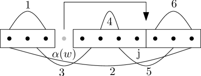
Figure 4: Illustration for the proof of Lemma 3.5

Lemma 3.5.

Let $1\leq j<n$ and let $w\in V$ be an isolated vertex such that $\alpha(w)<j$ and $|{\delta({X_{k}})}|\leq|{\delta({X_{j}})}|$ for all $\alpha(w)\leq k\leq j$. Then for the ordering $\alpha^{\prime}:V\rightarrow\{1,\dotsc,n\}$ defined by

$$\alpha^{\prime}(v)=\begin{cases}\alpha(v)&\text{if $\alpha(v)<\alpha(w)$ or $j<\alpha(v)$}\\ j&\text{if $v=w$}\\ \alpha(v)-1&\text{if $\alpha(w)<\alpha(v)\leq j$}\end{cases}$$

we have $\text{q}(\alpha^{\prime})\geq\text{q}(\alpha)$.

For an edge $e=(u,v)\in E$ we may assume that $\alpha(u)<\alpha(v)$. We denote the contribution of an edge $e$ to the change of cost by $\Delta(e)\mathrel{\mathop{:}}=\phi_{\alpha^{\prime}}(e)-\phi_{\alpha}(e)$. Based on the positions of $u$ and $v$ in $\alpha$ relative to $\alpha(w)$ and $j$, we now calculate $\Delta(e)$; there are six cases to be considered (see Fig. 4).

$$\alpha(u)<\alpha(v)<\alpha(w) \Rightarrow\Delta(e)=0$$

$$\alpha(u)<\alpha(w)\wedge j<\alpha(v) \Rightarrow\Delta(e)=0$$

$$\alpha(u)<\alpha(w)<\alpha(v)\leq j \Rightarrow\Delta(e)=-(2\alpha(v)+c-1)$$

$$\alpha(w)<\alpha(u)<\alpha(v)\leq j \Rightarrow\Delta(e)=+(2\alpha(u)+c-1)-(2\alpha(v)+c-1)$$

$$\alpha(w)<\alpha(u)\leq j<\alpha(v) \Rightarrow\Delta(e)=+(2\alpha(u)+c-1)$$

$$j<\alpha(u)<\alpha(v) \Rightarrow\Delta(e)=0$$

We now quantify the global change of cost. For accounting purpose, it is useful to associate a change of cost $\pm(2\alpha(x)+c-1)$ with the vertex $x$ (all cost changes are of that form). Notice that only vertices $x\in V$ with $\alpha(w)<\alpha(x)\leq j$ can have associated a change of cost with them. Moving from the $j$-th position in the arrangement to the left back to position $\alpha^{-1}(w)+1$, we pick up a positive change at vertex $x$ if and only if $|{\delta({X_{\alpha(x)}})}|>|{\delta({X_{\alpha(x)-1}})}|$ and a negative change if and only if $|{\delta({X_{\alpha(x)}})}|<|{\delta({X_{\alpha(x)-1}})}|$. If the size of the cut does not change at $x$, neither does the cost change (changes may cancel at that vertex though).

Since none of the cuts on the left of $j$ exceeds the size of the cut $\delta({X_{j}})$ and the absolute value of each change is strictly decreasing as we move to the left, the sum of accumulated changes stays non-negative throughout until we reach position $\alpha(w)+1$. But by reaching that position we have accounted for all changes due to the reordering, so we have $\text{q}(\alpha^{\prime})\geq\text{q}(\alpha)$.

Lemma 3.5 describes circumstances that allow moving a single isolated vertex from the left into a locally largest cut without decreasing the arrangement costs. Unfortunately, moving isolated vertices from the right of that cut is not as easy. In fact the cost can decrease if we move such a single isolated vertex in a position where it intersperses the cutarxiv (see Appendix B). But there are conditions under which we can move a block of isolated vertices from the right as the following lemma shows.

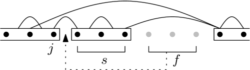
Figure 5: Illustration for the proof of Lemma 3.6. Edges symbolize the edge classes $E_{i}$.

Lemma 3.6.

Let $j,s,f\in\mathbb{N}$ be such that $1\leq j<j+s<j+s+f\leq n$, $|{\delta({X_{j}})}|>|{\delta({X_{j+k}})}|$ for $1\leq k\leq s+f$ and $\{\alpha^{-1}(j+s+1),\dotsc,\alpha^{-1}(j+s+f)\}\subset V$ are isolated vertices. Define the ordering $\alpha^{\prime}$ by

$$\alpha^{\prime}(v)=\begin{cases}\alpha(v)&\text{if $\alpha(v)\leq j$ or $\alpha(v)>j+s+f$}\\ \alpha(v)-s&\text{if $j+s<\alpha(v)\leq j+s+f$}\\ \alpha(v)+f&\text{if $j<\alpha(v)\leq j+s$}.\end{cases}$$

If $j+1+\frac{c+f}{2}\geq|{\delta({X_{j+s+f}})}|(s-1)$ then we have $\text{q}(\alpha^{\prime})\geq\text{q}(\alpha)$.

As in Lemma 3.5 we denote the change of cost when passing from $\alpha$ to $\alpha^{\prime}$ for an edge $e=(u,v)\in E$ by $\Delta(e)$ and we assume that $\alpha(u)<\alpha(v)$. Based on the positions of the end points, the edges can be divided into six disjoint sets (see Fig. 5):

$$E_{1} \mathrel{\mathop{:}}=\{(u,v)\in E\mid\alpha(u)<\alpha(v)\leq j\}$$

$$E_{2} \mathrel{\mathop{:}}=\{(u,v)\in E\mid\alpha(u)\leq j\wedge j+s+f<\alpha(v)\}$$

$$E_{3} \mathrel{\mathop{:}}=\{(u,v)\in E\mid\alpha(u)\leq j<\alpha(v)\leq j+s\}$$

$$E_{4} \mathrel{\mathop{:}}=\{(u,v)\in E\mid j<\alpha(u)<\alpha(v)\leq j+s\}$$

$$E_{5} \mathrel{\mathop{:}}=\{(u,v)\in E\mid j<\alpha(u)\leq j+s<j+s+f<\alpha(v)\}$$

$$E_{6} \mathrel{\mathop{:}}=\{(u,v)\in E\mid j+s+f<\alpha(u)<\alpha(v)\}$$

From the definition of $\alpha^{\prime}$, we see that $\Delta(e)=0$, for $e\in E_{1}\cup E_{2}\cup E_{6}$. For the other three cases a short calculation shows that

$$e\in E_{3}\Rightarrow\Delta(e) =f(2\alpha(v)+c+f),$$

$$e\in E_{4}\Rightarrow\Delta(e) =2f(\alpha(v)-\alpha(u))\quad\text{and}$$

$$e\in E_{5}\Rightarrow\Delta(e) =-f(2\alpha(u)+c+f).$$

We now derive a lower bound for the cost difference of $\alpha^{\prime}$ and $\alpha$. We will use that

$$|{E_{3}}|-|{E_{5}}|=|{E_{3}}|+|{E_{2}}|-(|{E_{5}}|+|{E_{2}}|)=|{\delta({X_{j}})}|-|{\delta({X_{j+s+f}})}|\geq 1,$$

as well as $|{E_{5}}|\leq|{\delta({X_{j+f+s}})}|$. We immediately drop the non-negative contribution from edges in $E_{4}$ and calculate

$$\begin{split}\text{q}(\alpha^{\prime})-\text{q}(\alpha)&\geq\sum_{(u,v)\in E_{3}}f(2\alpha(v)+c+f)-\sum_{(u,v)\in E_{5}}f(2\alpha(u)+c+f)\\ &\geq|{E_{3}}|f(2(j+1)+c+f)-|{E_{5}}|f(2(j+s)+c+f^{2})\\ &=(|{E_{3}}|-|{E_{5}}|)f(2(j+1)+c+f)-|{E_{5}}|2f(s-1)\\ &\geq f(2(j+1)+c+f)-|{\delta({X_{j+s+f}})}|2f(s-1)\\ &=f(2(j+1)+c+f-|{\delta({X_{j+s+f}})}|2(s-1)).\end{split}$$

By assumption we have $j+1+\frac{c+f}{2}\geq|{\delta({X_{j+s+f}})}|(s-1)$, so the difference $\text{q}(\alpha^{\prime})-\text{q}(\alpha)$ is non-negative.

Theorem 3.7.

Let $c=c_{2}X^{2}+c_{1}X+c_{0}$ be a polynomial of degree at most two with non-negative integer coefficients. Then ${\textsc{MaxCut}}\propto{\textsc{OQA}}(c)$.

Let $(G^{\prime}=(V^{\prime},E^{\prime});k^{\prime})$ be an instance of MaxCut. We define an instance $(G=(V,E);k)$ for OQA by adding $n^{5}$ isolated vertices to $G^{\prime}$: Let $W$ be set of size $n^{5}$, then we set

$$V=V^{\prime}\cup W,\quad E=E^{\prime}\quad\text{and}\quad k=n^{10}k^{\prime}.$$

Assume that $G^{\prime}$ admits a cut $\delta({X^{\prime}})$ of size at least $k^{\prime}$. We define an ordering $\alpha:V\rightarrow\{1,\dotsc,n+n^{5}\}$ for $G$ by

$$\begin{split}\alpha(X^{\prime})&=\{1,\dotsc,|{X^{\prime}}|\}\\ \alpha(W)&=\{|{X^{\prime}}|+1,\dotsc,|{X^{\prime}}|+n^{5}\}\\ \alpha(V^{\prime}\setminus X^{\prime})&=\{|{X^{\prime}}|+n^{5}+1,\dotsc,n^{5}+n\},\end{split}$$

where the ordering within the sets $X^{\prime},W$ and $V\setminus X^{\prime}$ is arbitrary. We now derive a lower bound for $\text{q}(\alpha)$: Every edge $e\in\delta({X^{\prime}})$ induces a cost of at least

$$\begin{split}\phi(e)&\geq(n^{5}+2)^{2}+c(n^{5}+2)-1^{2}-c\cdot 1\\ &=n^{10}+(4+c)n^{5}+c+3,\end{split}$$

so

$$\begin{split}\text{q}(\alpha)&=\sum_{e\in E}\phi(e)\geq\sum_{e\in\delta({X^{\prime}})}\phi(e)\geq(n^{10}+(4+c)n^{5}+c+3)|{\delta({X^{\prime}})}|\\ &\geq n^{10}k^{\prime}=k.\end{split}$$

For the reverse direction assume that we are given an ordering $\alpha:V\rightarrow\{1,\dotsc,n+n^{5}\}$ such that $\text{q}(\alpha)\geq k$. In order to show that $G^{\prime}$ has a cut of size at least $k^{\prime}$, we will first rearrange $\alpha$, without decreasing the ordering cost, so that the vertices in $W$ are ordered consecutively. This reordering process has two stages: First, using Lemma 3.5, we will move isolated vertices to the right so that they intersperse with locally largest cuts. This yields a block structure of isolated vertices of $W$ to which we will then apply Lemma 3.6 in a second step.

For the first stage, let $b_{1}$ be the largest index of a maximum cut among the cuts $\delta({X_{i}})$, that is,

$$b_{1}=\max\{\operatorname*{arg\,max}_{1\leq i\leq n^{5}+n}|{\delta({X_{i}})}|\}.$$

Among the $b_{1}$ vertices in $X_{b_{1}}$ denote by $n_{1}$ the number of vertices from $V^{\prime}$ and by $f_{1}$ the number of vertices from W, so $n_{1}=b_{1}+f_{1}$. By Lemma 3.5, we can rearrange $\alpha$ so that $\alpha^{-1}(\{1,\dotsc,n_{1}\})\subseteq V\setminus W$ and $\alpha^{-1}(\{n_{1}+1,\dotsc,n_{1}+f_{1}\})\subseteq W$ without decreasing the cost.

Iterating this procedure on the vertices ordered after $b_{1}$, we obtain an ordering in which the vertices appear partitioned in $h$ parts, where in each part the vertices of $V^{\prime}$ and $W$ are ordered consecutively (see Fig. 6). More formally, the ordering has the following properties:

$$0=\mathrel{\mathop{:}}b_{0}<b_{1}<b_{2}<\dotsb<b_{h}=n+n^{5},$$

$$b_{k}=\max\{\operatorname*{arg\,max}_{b_{k-1}<i\leq n^{5}+n}|{\delta({X_{i}})}|\},\quad 1\leq k\leq h,$$

$$|{\delta({X_{b_{1}}})}|>|{\delta({X_{b_{2}}})}|>\dotsb>|{\delta({X_{b_{h}}})}|=0,$$

$$n_{k}+f_{k}=b_{k}-b_{k-1},\quad 1\leq k\leq h,$$

$$\sum n_{k}=n,\quad\sum f_{k}=n^{5},$$

$$\alpha^{-1}(\{b_{k-1}+1,\dotsc,b_{k-1}+n_{k}\})\subseteq V\setminus W,\quad 1\leq k\leq h,$$

$$\alpha^{-1}(\{b_{k-1}+n_{k}+1,\dotsc,b_{k-1}+n_{k}+f_{k}\})\subseteq W,\quad 1\leq k\leq h$$

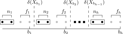
Figure 6: Illustration for the block structure arising from moving isolated vertices closest to their rightmost largest cut.

Note that some of the $f_{k}$ may be zero but all $n_{k}>0$. Since $|{\delta({X_{b_{1}}})}|$ is trivially bounded by the linear cutwidth of the complete graph on $n$ vertices and the size of the cuts $\delta({X_{k}})$ is strictly decreasing, we obtain $h\leq\frac{n^{2}}{4}$.

Now begins the second stage of the rearrangement. From the given block structure, we will perform a series of rearrangements using Lemma 3.6 until eventually all vertices from $W$ intersperse between the sets $X_{b_{1}}$ and $\overline{X_{b_{1}}}$. Each of the reordering operations will maintain the block structure as a whole, but the individual values of the $f_{k}$ will change. In order to simplify notation, we will not explicitly distinguish between different orderings $\alpha$ and values $f_{k}$’s at the different stages during the process.

Let $\nu\in\operatorname*{arg\,max}_{1\leq k\leq h}f_{k}$; since $\sum f_{k}=n^{5}$ and $h\leq\frac{n^{2}}{4}$, we have $f_{\nu}\geq 4n^{3}$. Define $j\mathrel{\mathop{:}}=b_{\nu-1},s\mathrel{\mathop{:}}=n_{\nu},f\mathrel{\mathop{:}}=f_{\nu}$. By construction we have that $|{\delta({X_{j}})}|>|{\delta({X_{j+k}})}|$ for $1\leq k\leq s+f$ and

$$j+1+\frac{c+f}{2}\geq\frac{f}{2}\geq 2n^{3}\geq\frac{n^{2}}{4}(n-1)\geq|{\delta({X_{j+s+f}})}|(s-1).$$

So the assumptions of Lemma 3.6 are met and in the rearranged ordering we now have $f_{\nu-1}\geq 4n^{3}$ and $f_{\nu}=0$. By induction we obtain an ordering in which the block structure satisfies $f_{1}\geq 4n^{3}$ and $f_{2}=\dotsb=f_{\nu}=0$.

Next set $j\mathrel{\mathop{:}}=b_{1}\geq 4n^{3}$, $s\mathrel{\mathop{:}}=\sum_{k=2}^{\nu}(n_{k}+f_{k})+n_{\nu+1}=\sum_{k=2}^{\nu+1}n_{k}\leq n$ and $f\mathrel{\mathop{:}}=f_{\nu+1}$. By construction we have that $|{\delta({X_{j}})}|>|{\delta({X_{j+k}})}|$ for $1\leq k\leq s+f$ and

$$j+1+\frac{c+f}{2}\geq j\geq 4n^{3}\geq\frac{n^{2}}{4}(n-1)\geq|{\delta({X_{j+s+f}})}|(s-1).$$

This permits us to apply Lemma 3.6 and in the rearranged ordering we now have $f_{\nu+1}=0$ while $f_{1}\geq 4n^{3}$ is maintained. By induction we arrive at an ordering where $f_{2}=\dotsb=f_{h}=0$, which implies $f_{1}=n^{5}$. Denote this final ordering by $\alpha^{\prime}$. Since none of the reordering operations has ever decreased the total arrangement cost, we have $\text{q}(\alpha^{\prime})\geq\text{q}(\alpha)\geq k$, where $\alpha$ is the very original ordering that we started with.

Next we derive an upper bound for $\text{q}(\alpha^{\prime})$. We classify the edges of $G$ in three different categories and bound the contribution from each of these sources.

1. If $(u,v)\in X_{1}\times X_{1}$, then the total cost of these edges is strictly bounded by the arrangement cost of a clique of size $n$ being ordered at positions $1,\dotsc,n$. By Lemma 3.3 (with $r=0$), this cost is $\frac{1}{6}n(n^{2}-1)(c+n+1)$.

2. If $e=(u,v)\in X_{1}\times\overline{X_{1}}$, then the cost implied by $e$ is at most $(n^{5}+n)^{2}+c(n^{5}+n)-1^{2}-c$.

3. If $(u,v)\in\overline{X_{1}}\times\overline{X_{1}}$, then the total cost of these edges is strictly bounded by the arrangement cost of a clique of size $n$ being ordered at positions $n^{5}+1,\dotsc,n^{5}+n$. By Lemma 3.3, this cost is $\frac{1}{6}n(n^{2}-1)(2n^{5}+c+n+1)$.

In total we obtain

$$n^{10}k^{\prime} =k\leq\text{q}(\alpha)\leq\text{q}(\alpha^{\prime})$$

$$\leq|{\delta({X_{1}})}|((n^{5}+n)^{2}+c(n^{5}+n)-1-c)+\frac{n}{6}(n^{2}-1)(c+n+1)$$

$$\quad+\frac{n}{6}(n^{2}-1)(2n^{5}+c+n+1)$$

$$\leq|{\delta({X_{1}})}|(n^{10}+2n^{6}+cn^{5}+n^{2}+cn)+\frac{1}{3}n(n^{2})(n^{5}+c+n+1)$$

$$\Rightarrow k^{\prime}\leq|{\delta({X_{1}})}|+\underbrace{|{\delta({X_{1}})}|\frac{2n^{6}+cn^{5}+n^{2}+cn}{n^{10}}+\frac{n^{8}+cn^{3}+n^{4}+n^{3}}{3n^{10}}}_{=\mathrel{\mathop{:}}r(n)}.$$

Since $|{\delta({X_{1}})}|\leq\frac{n^{2}}{4}$, we have

$$r(n)\leq\frac{1}{2n^{2}}+\frac{c}{4n^{3}}+\frac{1}{4n^{6}}+\frac{c}{4n^{7}}+\frac{1}{3n^{2}}+\frac{c}{3n^{7}}+\frac{1}{3n^{6}}+\frac{1}{3n^{7}}.$$

Because $c$ is a polynomial of degree at most two, there exists an integer $n_{c}\in\mathbb{N}$ such that

$$r(n)<1,\quad\text{for all}\quad n\geq n_{c}.$$

Together with the integrality of $|{\delta({X_{1}})}|$ and $k^{\prime}$, it follows that $|{\delta({X_{1}})}|\geq k^{\prime}$.

3.2 Reduction from OQA to the minimum FLOPs problem

In this section we reduce OQA(c) to the minimum FLOPs problem for a certain polynomial $c$. Our strategy follows the pattern that Yannakakis used for the reduction of OLA to minimum fill [24], but again the details are much different. In particular we employ a quadratic variation of the bipartite chain graph completion problem, which we discuss in section 3.2.1. In section 3.2.2 we give a reduction from OQA(c) to this quadratic chain completion problem.

3.2.1 Reduction from bipartite quadratic chain completion

Let $G=(P,Q,E)$ be a bipartite graph on $p+q$ vertices, $p\mathrel{\mathop{:}}=|{P}|,q\mathrel{\mathop{:}}=|{Q}|$. Recall that for a vertex $v\in P$ we denote its neighbourhood in $G$ by $\mathcal{N}\left(v\right)$. $G$ is a bipartite chain graph if there exists a bijection $\alpha:P\rightarrow\{1,\dotsc,p\}$ such that

$$\mathcal{N}\left(\alpha^{-1}(i)\right)\supseteq\mathcal{N}\left(\alpha^{-1}(i+1)\right),\;1\leq i\leq p-1.$$ (8)

Note that $G$ admits such a chain ordering for $P$ if and only if $G$ admits a chain ordering for $Q$, so the definition does not depend on a particular partition of $G$. For a bipartite graph, the property of being a chain graph is hereditary and the minimal obstruction set is $\{2K_{2}\}$ [24, Lemma 1].

Yannakakis considers the problem of completing a given bipartite graph into a bipartite chain graph. We formulate the corresponding decision problem in terms of vertex degrees:

BipartiteChainCompletion (BCC)
Instance: Bipartite graph $G=(P,Q,E),k\in\mathbb{N}$ Question: Is there a set of edges $F\subseteq P\times Q$ such that $G^{+}=(P,Q,E\cup F)$ is a chain graph and $\sum_{v\in P}\mbox{d}_{G^{+}}(v)\leq k$ ?

Note that our metric of measuring the cost of the chain completion is equivalent to minimizing $|{F}|$ in the formulation above, because

$$\sum_{v\in P}\mbox{d}_{G^{+}}(v)=|{E}|+|{F}|.$$

Our quadratic variation of the bipartite chain completion problem has a cost function which is a quadratic function of the vertex degrees in the augmented graph.

QuadraticChainCompletion (QCC)
Instance: Bipartite graph $G=(P,Q,E)$ on $p+q$ vertices ($p=|{P}|$, $q=|{Q}|$) where the partition $P$ is designated, $k\in\mathbb{N}$ Question: Is there a set of edges $F\subseteq P\times Q$ such that $G^{+}=(P,Q,E\cup F)$ is a chain graph with $$\text{qcc}(F)\mathrel{\mathop{:}}=\sum_{v\in P}\mbox{d}_{G^{+}}(v)^{2}+2(p+1)\sum_{v\in P}\mbox{d}_{G^{+}}(v)\leq k?$$

Unlike for BCC, it is not clear whether the minima of our quadratic variation depend on the particular vertex partition chosen, which is why the information which partition to consider is part of the input. Of course, the particular cost value (defined by qcc) of a bipartite chain graph embedding depends on the partition (for example, consider the simple path on three vertices).

The reduction from BCC to MinimumFill in [24] involves a construction that relates certain triangulations to chain embeddings, which we adapt to our needs by augmenting it with an additional vertex set $U$:

Definition 3.8.

Let $G=(P,Q,E)$ a bipartite graph on $p+q$ vertices and $U=\{u_{v}\mid v\in P\}$ a set of $p$ vertices. We define the graph $C=C(G)=(V^{\prime},E^{\prime})$ by

$$V^{\prime} =P\cup Q\cup U$$

$$E^{\prime} =E\cup(P\times P)\cup((Q\cup U)\times(Q\cup U))\cup\{(v,u_{v})\mid v\in P\}.$$

Further, for a given bijection $\alpha:P\rightarrow\{1,\dotsc,p\}$, we define the set

$$G(\alpha)=\{(\alpha^{-1}(i),u_{\alpha^{-1}(j)})\mid 1\leq i<j\leq p\}\subset P\times U.$$

(a) $G=(P,Q,E)$

(b) $C=C(G)$

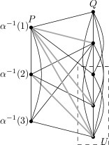
(c) $C^{+}$, a triangulation of $C$

Figure 7: Illustration for the reduction from QCC to minimum FLOPs. Figs. 7(a) and 7(b) show the construction of $C(G)$. Notice that the two topmost vertices of $P$ and the vertices of $Q$ induce a $2K_{2}$ in $G$ and a chordless cycle in $C$. Fig. 7(c) shows a triangulation of $C$; the fill edges are shown in gray. The topmost fill edge turns $G$ into a chain graph with $P$-chain ordering $\alpha$, the other three fill edges constitute $G(\alpha)$. $\alpha^{R}$ is a prefix of a PEO for $C^{+}$.

Figs. 7(a) and 7(b) give an example for the construction of $C(G)$. The next lemmas describe how chain completions of $G$ relate to triangulations of $C(G)$ and $G(\alpha)$, giving an analogon to [24, Lemma 2]. Fig. 7(c) illustrates this relationship.

Definition 3.9.

Let $M$ be a set of $m$ elements and $\alpha:M\rightarrow\{1,\dotsc,m\}$ a bijection. Then the reverse bijection $\alpha^{R}:M\rightarrow\{1,\dotsc,m\}$ is uniquely defined by the property $\alpha^{-R}(i)\mathrel{\mathop{:}}=(\alpha^{R})^{-1}(i)=\alpha^{-1}(m-i+1)$ for $1\leq i\leq m$.

For the following we recall that a minimal triangulation for a graph is an inclusion minimal set of edges whose addition yields a chordal graph. Analogously we will speak of minimal chain completions for a given bipartite graph. There is no loss of generality if we assume that the decision problems from above are restricted to minimal completions. Recall also that a PEO for a graph $G=(V,E)$ is a bijection $\alpha:V\rightarrow\{1,\dotsc,n\}$, $n=|{V}|$, such that eliminating vertices in the order implied by $\alpha^{-1}$ does not cause any fill. By a prefix of a PEO $\alpha$ we mean a restriction $\alpha_{|_{W}}$ for some $W\subset V$ such that $\alpha^{-1}(k)=\alpha^{-1}_{|_{W}}(k)$, for $1\leq k\leq|{W}|$.

Lemma 3.10.

Let $G=(P,Q,E)$ be a bipartite graph, $C=C(G)=(V^{\prime},E^{\prime})=(P\cup Q\cup U,E^{\prime})$ and $F^{\prime}\subseteq V^{\prime}\times V^{\prime}$ a minimal triangulation of $C$. Set $F^{\prime}_{U}\mathrel{\mathop{:}}=F^{\prime}\cap(P\times U),F^{\prime}_{Q}\mathrel{\mathop{:}}=F^{\prime}\cap(P\times Q)$. Then there exists a bijection $\alpha:P\rightarrow\{1,\dotsc,p\}$ such that

1. $F^{\prime}_{U}=G(\alpha)$,

2. $(P,Q,E\cup F^{\prime}_{Q})$ is a chain graph and admits $\alpha$ as a chain ordering for $P$.

Since $P$ and $Q\cup U$ are already cliques in $C$, we have $F^{\prime}\subseteq P\times(Q\cup U)$, so $F^{\prime}=F_{U}^{\prime}\cup F_{Q}^{\prime}$ is a partitioning of $F^{\prime}$. Since $F^{\prime}$ is minimal, there exists a PEO $\beta$ for $C^{+}$ such that $C_{\beta}^{+}=C^{+}$, and because $Q\cup U$ is a clique in $C^{+}$, we can choose $\beta$ so that it orders $Q\cup U$ last [22, Corollary 4], that is,

$$\beta^{-1}(\{1,\cdots,p\})=P,\;\beta^{-1}(\{p+1,\cdots,2p+q\})=Q\cup U.$$

Denote by $N_{j}$ the neighborhood of the vertex $\beta^{-1}(j)$ in the reduced elimination graph at step $j$, and $F^{\prime}_{j}$ the set of fill edges introduced at step $j$ that are incident with $U$. We will show the following statement by induction (for $1\leq j\leq p$): In the $j$-th elimination step, we have

$$N_{j}\cap(P\cup U) =\{\beta^{-1}(i)\mid j<i\leq p\}\cup\{u_{\beta^{-1}(i)}\mid 1\leq i\leq j\},$$

$$F^{\prime}_{j} =\{(\beta^{-1}(i),u_{\beta^{-1}(j)})\mid j<i\leq p\}.$$

By inspection of the graph $C$ we find that the statement is true for $j=1$. Next assume that the statement is true for all $k$ with $1\leq k<j$. By the induction assumption, the fill edges incident with $U$ introduced up to step $j$ are

$$\bigcup_{k=1}^{j-1}F^{\prime}_{k}=\bigcup_{k=1}^{j-1}\{(\beta^{-1}(i),u_{\beta^{-1}(k)})\mid k<i\leq p\}.$$ (9)

So at the elimination step $j$, the set of vertices of $U$ that the vertex $\beta^{-1}(j)\in P$ is adjacent to because of any prior fill edge is $\{u_{\beta^{-1}(i)}\mid 1\leq i<j\}$, so we obtain

$$N_{j}\cap(P\cup U)=\{\beta^{-1}(i)\mid j<i\leq p\}\cup\{u_{\beta^{-1}(i)}\mid 1\leq i\leq j\}.$$

Since the edges (9) are already present at step $j$, the only edges that need to be added in order to turn this set of vertices into a clique

$$\{(\beta^{-1}(i),u_{\beta^{-1}(j)})\mid j<i\leq p\}=F^{\prime}_{j},$$

which completes the proof of the claim.

Let $\alpha\mathrel{\mathop{:}}=(\beta|_{P})^{R}$. Noting that $F^{\prime}_{p}=\emptyset$, it follows from the claim that

$$F^{\prime}\cap(P\times U) =\bigcup_{j=1}^{p-1}F^{\prime}_{k}=\bigcup_{j=1}^{p-1}\{(\beta^{-1}(i),u_{\beta^{-1}(j)})\mid j<i\leq p\}$$

$$=\{(\alpha^{-1}(i),u_{\alpha^{-1}(j)})\mid 1\leq i<j\leq p\}=G(\alpha).$$

Now we have constructed $\alpha$ and shown (i). To show (ii), note that $P$ is a clique in $C(G)$ and $\alpha^{R}=\beta|_{P}$ is also a prefix of a PEO for the induced subgraph $C^{+}[P\cup Q]$. So by the construction of $C$, $\alpha$ is a chain ordering for $P$ in in $(P,Q,E\cup F_{Q}^{\prime})$.

The previous lemma characterizes minimal triangulations of $C(G)$: They decompose into a chain completion for $G$ and a set $G(\alpha)$ such that $\alpha$ is a compatible chain ordering. The next two lemmas give a reverse direction, so every triangulation of $C(G)$ uniquely defines a chain completion of $G$ and vice versa.

Lemma 3.11 (chordal patching lemma, folklore).

Let $G=(V,E)$ be a graph where the vertices are partitioned in three disjoint sets $V=A\cup B\cup C$. Then $G$ is chordal if the following three conditions are satisfied:

1. $G[V\setminus C]$ has two connected components $A,B$,

2. $G[C]$ is a clique,

3. $G[A\cup C]$ and $G[B\cup C]$ are chordal.

Let $Z$ be a simple cycle of length at least $4$ in $G$. If $Z$ is entirely contained in $A\cup C$ or $B\cup C$, then $Z$ has a chord. Otherwise, $Z$ contains vertices both of $A$ and $B$, so $Z$ intersects $C$ at least at two non-consecutive vertices of $Z$, which gives a chord in $Z$ since $C$ is a clique.

Lemma 3.12.

Let $G=(P,Q,E)$ be a bipartite graph and let $F\subseteq P\times Q$ such that $G^{+}=(P,Q,E\cup F)$ admits $\alpha:P\rightarrow\{1,\dotsc,p\}$ as a chain ordering. Then $F^{\prime}=F\cup G(\alpha)$ is a triangulation for $C=C(G)=(V^{\prime},E^{\prime})$ and $\alpha^{R}$ is a prefix of a PEO for $C^{+}=(V^{\prime},E^{\prime}\cup F^{\prime})$.

Let $C^{+}_{Q}=C^{+}[P\cup Q]$ and $C^{+}_{U}=C^{+}[P\cup U]$. We first show that $C^{+}_{Q}$ and $C^{+}_{U}$ are chordal. A chordless cycle in $C^{+}_{Q}$ implies an induced subgraph in $G^{+}$ isomorphic to $2K_{2}$, which contradicts the assumption that $G^{+}$ is a bipartite chain graph. So $C^{+}_{Q}$ is chordal.

From the definition of $G(\alpha)$ it follows that we can use $\alpha^{R}$ to carry out $p$ steps of vertex elimination in $C^{+}_{U}$ without introducing a fill edge. But after these $p$ steps only a clique of size $p$ remains, so $C^{+}_{U}$ admits a PEO which implies that $C^{+}_{U}$ is chordal.

Noting that $P$ is a clique in $C^{+}$, it follows from Lemma 3.11 that $C^{+}$ is chordal. Since $G^{+}$ is a chain graph and since $P$ is a clique in $C^{+}$, no fill edge is introduced when eliminating along $\alpha^{R}$. Consequently, $\alpha^{R}$ is a prefix of a PEO for $C^{+}$.

The set $G(\alpha)$ in any triangulation $C^{+}$ of $C(G)$ simplifies the FLOP counting in the reduction from QuadraticChainCompletion as we will see now.

Theorem 3.13.

QuadraticChainCompletion $\propto$ MinimumFLOPs.

As before, we continue to use the notation from Definition 3.8. By Lemmas 3.10 and 3.12 every chain completion $F$ of $G$ gives a triangulation $F^{\prime}=F\cup G(\alpha)$ for $C(G)$ and vice versa. Further, the chain orderings correspond to reversed prefixes of PEOs and vice versa. We show: There exists a chain completion of cost at most $k$ if and only if we can triangulate $C(G)$ with FLOP count of at most $k^{\prime}\mathrel{\mathop{:}}=k+p(p+1)^{2}+\sum_{i=1}^{p+q}i^{2}$.

If $F$ is a set of edges whose addition to $G$ yields a chain graph $G^{+}$ with chain ordering $\alpha$ for $P$, then $\alpha^{R}$ starts a PEO for the corresponding triangulation of $C(G)$. We will calculate the elimination degrees. At the $i$-th elimination step, the vertex $\alpha^{R}(i)$ is adjacent to $p-i$ vertices in $P$, $\mbox{d}_{G^{+}}(\alpha^{R}(i))$ vertices in $Q$ and $i$ vertices in $U$. So the $p$ elimination degrees associated with $\alpha^{R}$ are

$$\begin{split}\mbox{d}(\alpha^{R}(i))&=p-i+\mbox{d}_{G^{+}}(\alpha^{R}(i))+i\\ &=p+\mbox{d}_{G^{+}}(\alpha^{R}(i)),\quad 1\leq i\leq p.\end{split}$$ (10)

After the elimination of these first $p$ vertices, a clique of size $p+q$ remains, so a PEO $\alpha^{\prime}$ for $C^{+}$ is obtained by completing $\alpha^{R}$ arbitrarily. For the FLOP count we find:

$$\text{flop}(\alpha^{\prime}) =\sum_{i=1}^{p}(p+1+\mbox{d}_{G^{+}}(\alpha^{R}(i)))^{2}+\sum_{i=1}^{p+q}i^{2}$$

$$=\sum_{v\in P}\mbox{d}_{G^{+}}(v)^{2}+2(p+1)\sum_{v\in P}\mbox{d}_{G^{+}}(v)+p(p+1)^{2}+\sum_{i=1}^{p+q}i^{2}$$

$$=\text{qcc}(F)+p(p+1)^{2}+\sum_{i=1}^{p+q}i^{2}.$$

Since the FLOP count does not depend on the particular PEO $\alpha^{\prime}$ for $C^{+}$, the FLOP count induced by the triangulation $F^{\prime}$ is less than $k^{\prime}$ if and only if the quadratic chain completion cost of $F$ is less than $k$.

If we would omit the vertices $U$ from the construction of $C(G)$, the vertex degrees (10) would depend on the position of the vertices in the ordering $\alpha$. The implied quadratic cost function for the chain completion problem would make the treatment that follows much more difficult.

3.2.2 Reduction from optimal quadratic arrangement

In section 3.1 we have shown that OQA($c$) is an NP hard problem for any choice of the polynomial $c$ in (7). For the rest of the section we are interested only in the special case OQA($2(X^{2}+1)$), which we reduce to the QCC problem. This polynomial is intentionally chosen to match up with the $2(p+1)$ factor in the formulation of the QCC problem.

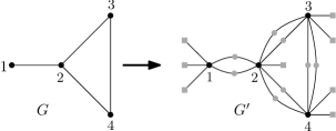
Figure 8: Illustration for the reduction from OQA to QCC. The gray vertices of $G^{\prime}$ form the partition $Q$. The vertices marked as squares correspond to the sets $R(v)$, and the gray discs correspond to the vertices $w_{i}^{e}$.

The following construction for creating a bipartite graph $G^{\prime}=(P,Q,E^{\prime})$ from a given graph $G=(V,E)$ on $n$ vertices is used in [24, Lemma 3]. For a vertex $v\in V$ define the set $R(v)\mathrel{\mathop{:}}=\{w^{v}_{1},\dotsc,w^{v}_{l_{v}}\mid l_{v}=n-\mbox{d}_{G}(v)\}$, then $G^{\prime}$ is given by (see Fig. 8)

$$\begin{split}P&=V,\quad Q=\{w^{e}_{1},w^{e}_{2}\mid e\in E\}\bigcup_{v\in V}R(v)\quad\text{and}\\ E^{\prime}&=\{(u,w^{e}_{i})\mid e\in E,u\in V,e\in\delta({u}),1\leq i\leq 2\}\\ &\quad\cup\{(v,w)\mid v\in V,w\in R(v)\}.\end{split}$$ (11)

The construction of $G^{\prime}$ is such that all inclusion minimal chain completions can be easily characterized from vertex orderings of $G$, as the next lemma shows.

Lemma 3.14 (extracted from [24, Lemma 3]).

Let $\alpha:V\rightarrow\{1,\dotsc,n\}$ be an ordering for the vertices of $G=(V,E)$ and for $w\in Q$, define $\sigma(w)=\max\{i\mid(w,\alpha^{-1}(i))\in E^{\prime}\}$. Then

$$H(\alpha)=\{(\alpha^{-1}(j),w)\mid w\in Q,j<\sigma(w)\}\setminus E^{\prime}\subseteq P\times Q$$ (12)

is a set of edges whose addition to $G^{\prime}$ yields a bipartite chain graph with chain ordering $\alpha$ for $P$. Moreover, for any minimal set of edges $F$ such that $(P,Q,E^{\prime}\cup F)$ is a bipartite chain graph with $P$-ordering $\alpha$, we have $F=H(\alpha)$.

Theorem 3.15.

Let $c=2(X^{2}+1)$, then OQA(c) $\propto$ QCC.

Let $(G=(V,E);k)$ be an instance of OQA with $|{V}|=n,|{E}|=m$. Let $G^{\prime}$ be constructed as in (11). We define an instance for QCC by $(G^{\prime};k+p(n))$, where $p(n)=\frac{1}{6}n^{2}(n+1)(2n+3c(n)+1)$, and regard $Q$ as the designated partition for the decision problem. For the number of vertices in $Q$ we find

$$|{Q}|=2m+\sum_{v\in V}|{R(v)}|=2m+\sum_{v\in V}n-\mbox{d}_{G}(v)=2m+n^{2}-2m=n^{2}.$$

By Lemma 3.14, we only need to relate the quadratic ordering cost of an arbitrary vertex ordering $\alpha:V\rightarrow\{1,\dotsc,n\}$ for $G$ to the quadratic chain completion cost for $H(\alpha)$ for $G^{\prime}$. Set $G^{\prime+}=(P,Q,E^{\prime}\cup H(\alpha))$ and assume for all edges $e=(u,v)\in E$ that we have $\alpha(u)<\alpha(v)$. For every vertex $w^{e}_{i}\in Q$, we have $\mbox{d}_{G^{\prime+}}(w^{e}_{i})=\alpha(v)$. For any $v\in V$ we have $\mbox{d}_{G^{\prime+}}(w)=\alpha(v)$ for all vertices $w\in R(v)$. We abbreviate $l_{v}\mathrel{\mathop{:}}=n-\mbox{d}_{G}(v)$ and find for the total quadratic chain completion cost:

$$\text{qcc}(H(\alpha))=\sum_{w\in Q}(\mbox{d}_{G^{\prime+}}(w)^{2}+\underbrace{2(n^{2}+1)}_{=c(n)}\mbox{d}_{G^{\prime+}}(w))$$

$$=2\sum_{(u,v)\in E}(\alpha(v)^{2}+c(n)\alpha(v))+\sum_{v\in V}\sum_{x\in R(v)}(\alpha(v)^{2}+c(n)\alpha(v))$$

$$=2\sum_{(u,v)\in E}(\alpha(v)^{2}+c(n)\alpha(v))+\sum_{v\in V}(n-\mbox{d}_{G}(v))(\alpha(v)^{2}+c(n)\alpha(v))$$

$$\quad+\sum_{(u,v)\in E}(\alpha(u)^{2}+c(n)\alpha(u))-\sum_{(u,v)\in E}(\alpha(u)^{2}+c(n)\alpha(u))$$

$$=\sum_{(u,v)\in E}(\alpha(v)^{2}-\alpha(u)^{2}+c(n)(\alpha(v)-\alpha(u)))$$

$$\quad+\sum_{(u,v)\in E}(\alpha(v)^{2}+\alpha(u)^{2}+c(n)(\alpha(u)+\alpha(v))+\sum_{v\in V}l_{v}(\alpha(v)^{2}+c(n)\alpha(v))$$

$$=\text{q}(\alpha)+\sum_{v\in V}\mbox{d}_{G}(v)(\alpha(v)^{2}+c(n)\alpha(v))+\sum_{v\in V}(n-\mbox{d}_{G}(v))(\alpha(v)^{2}+c(n)\alpha(v))$$

$$=\text{q}(\alpha)+n\sum_{v\in V}(\alpha(v)^{2}+c(n)\alpha(v))=\text{q}(\alpha)+p(n).$$

This shows $\text{q}(\alpha)\leq k\Leftrightarrow\text{qcc}(H(\alpha))\leq k+p(n)$, which completes the proof.

Taken together, the three reductions in this section imply that it is NP hard to minimize the number of arithmetic operations in the sparse Cholesky factorization.

4 Conclusions and future work

In this work we have shown by means of an explicit, scalable construction that minimum fill and minimum operation count for the sparse Cholesky factorization are not achievable simultaneously in general. We proved that minimizing the number of arithmetic operations is just as difficult as minimizing the fill: it is NP hard. While this result is not surprising, no proof has been given so far, and thus our findings close a gap in the theoretical body of sparse direct methods.

It would be of interest to understand how well optimal fill orderings approximate the optimal number of arithmetic operations (and vice versa). Approximation bounds based on general equivalence constants for the 1- and 2-norm or bounds based on full $k$-tree embeddings (e.g. [22, prop. 3]) are too coarse for offering an quantitative insight into this question.

Acknowledgements

We would like to thank Tim Davis and John Gilbert for inspiring discussions at a Dagstuhl workshop which encouraged this work. We are also grateful to two anonymous referees for their useful suggestions.

Research at Lawrence Berkeley National Laboratory was supported by the Office of Advanced Scientific Computing Research of the US Department of Energy under contract number DE-AC02-05CH11231.

arxiv

Appendix A OQA(c) and OLA are different

We show that OLA and OQA are different problems in the sense that optimizing the linear arrangement cost does not necessarily optimize the quadratic arrangement cost (and vice versa). Let $n>4$, $C$ a set of size $n$, $u,v\in C$ two distinct elements and consider the following class of graphs $G=(V,E)$ (see Fig. 9):

$$V=C\cup\{x,y\},\quad E=C\times C\cup\{(x,u),(y,v)\}$$

Figure 9: A graph where minimum quadratic- and linear arrangement costs are attained on distinct orderings.

It is easy to see that any linear or quadratic arrangement where $x$ or $y$ intersperses with the vertices of $C$ is suboptimal. If $x,y$ are ordered before or after $C$, any ordering that does not place $u,v$ as close as possible to $x,y$ is suboptimal, too. Ruling out those suboptimal orderings, only five different orderings (modulo cost-neutral rearrangements of $C$) remain; they are displayed in Fig. 9 on the right. We calculate the linear arrangement costs:

$$\text{l}(\alpha_{1})=\frac{1}{6}n(n^{2}-1)+2,\quad\text{l}(\alpha_{2/3})=\text{l}(\alpha_{4/5})=\frac{1}{6}n(n^{2}-1)+4,$$

so $\alpha_{1}$ is an optimal linear arrangement while the others are not. Using Lemma 3.3 we find the quadratic arrangement costs

$$\text{q}(\alpha_{1}) =\frac{1}{6}n(n^{2}-1)(c+n+3)+2n+c+3,$$

$$\text{q}(\alpha_{2/3}) =\frac{1}{6}n(n^{2}-1)(c+n+5)+4c+20,$$

$$\text{q}(\alpha_{4/5}) =\frac{1}{6}n(n^{2}-1)(c+n+1)+8n+4c+4.$$

It is easy to see that $\text{q}(\alpha_{4/5})$ is strictly less than the other costs for sufficiently large $n$ (recall that $c$ is fixed). Thus OQA and OLA are different problems for every polynomial $c$.

Appendix B Moving isolated vertices to the left

In the reduction from MaxCut to OQA(c), we needed to rearrange isolated vertices within a given ordering without decreasing the costs. Fig. 10 shows an arrangement of a graph on 8 vertices, of which one is isolated. If the isolated vertex is moved to the left so that it intersperses with the largest cut, the arrangement cost decreases. This is why we need to resort to rearranging blocks of isolated vertices.

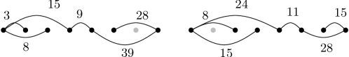
Figure 10: Moving an isolated vertex to the left into the largest cut may decrease the total arrangement cost. The numbers shown next to the edges are the edge costs; the arrangement on the left has a total cost of 102 while the arrangement on the right has cost 101. Here the distance function is $f(x)=x^{2}$.

Appendix C Auxiliary proofs

Proof of Lemma 3.3

We shall first proof the lemma with $r=0$. We say that the vertices $u,v$ have ordering distance $d$, $1\leq d\leq s-1$, if $|\alpha(u)-\alpha(v)|=d$. The cost implied by all edges between vertices of ordering distance $d$ is

$$\begin{split}&\quad\sum_{k=1}^{s-d}\left((k+d)^{2}+c(k+d)-k^{2}-ck\right)=2d\sum_{k=1}^{s-d}k+d(d+c)(s-d)\\ &=d(s-d)(s-d+1)+d(d+c)(s-d)=d(c+s+1)(s-d).\end{split}$$

The total cost of $\alpha$ is the sum over all the distances $1\leq d\leq s-1$, so we find

$$\begin{split}\text{q}(\alpha)&=\sum_{d=1}^{s-1}d(c+s+1)(s-d)=(c+s+1)(s\sum_{d=1}^{s-1}d-\sum_{d=1}^{s-1}d^{2})\\ &=(c+s+1)(\frac{1}{2}s^{2}(s-1)-\frac{1}{6}s(s-1)(2s-1))\\ &=\frac{1}{6}s(s^{2}-1)(c+s+1).\end{split}$$

Application of the translation lemma to the above cost finishes the proof.

References

- [1] Ajit Agrawal, Philip Klein, and R. Ravi. Cutting down on fill using nested dissection: provably good elimination orderings. In Graph theory and sparse matrix computation, volume 56 of IMA Vol. Math. Appl., pages 31–55. Springer, New York, 1993.
- [2] Patrick R. Amestoy, Timothy A. Davis, and Iain S. Duff. An approximate minimum degree ordering algorithm. SIAM J. Matrix Anal. Appl., 17(4):886–905, 1996.
- [3] Patrick R. Amestoy, Timothy A. Davis, and Iain S. Duff. Algorithm 837: AMD, an approximate minimum degree ordering algorithm. ACM Trans. Math. Software, 30(3):381–388, 2004.
- [4] Stefan Arnborg, Derek G. Corneil, and Andrzej Proskurowski. Complexity of finding embeddings in a -tree. SIAM J. Algebraic Discrete Methods, 8(2):277–284, 1987.
- [5] Hans L. Bodlaender, John R. Gilbert, Hjálmtýr Hafsteinsson, and Ton Kloks. Approximating treewidth, pathwidth, frontsize, and shortest elimination tree. J. Algorithms, 18(2):238–255, 1995.
- [6] Timothy A. Davis and Yifan Hu. The University of Florida sparse matrix collection. ACM Trans. Math. Software, 38(1):Art. 1, 25, 2011.
- [7] I. S. Duff and J. K. Reid. The multifrontal solution of indefinite sparse symmetric linear equations. ACM Trans. Math. Software, 9(3):302–325, 1983.
- [8] I. S. Duff and J. K. Reid. A note on the work involved in no-fill sparse matrix factorization. IMA J. Numer. Anal., 3(1):37–40, 1983.
- [9] Shimon Even. Graph algorithms. Computer Science Press Inc., Woodland Hills, Calif., 1979. Computer Software Engineering Series.
- [10] Michael R. Garey and David S. Johnson. Computers and intractability. W. H. Freeman and Co., San Francisco, Calif., 1979. A guide to the theory of NP-completeness, A Series of Books in the Mathematical Sciences.
- [11] Alan George and Joseph W. H. Liu. The evolution of the minimum degree ordering algorithm. SIAM Rev., 31(1):1–19, 1989.
- [12] Alan George and Alex Pothen. An analysis of spectral envelope reduction via quadratic assignment problems. SIAM J. Matrix Anal. Appl., 18(3):706–732, 1997.
- [13] Pinar Heggernes. Minimal triangulations of graphs: a survey. Discrete Math., 306(3):297–317, 2006.
- [14] George Karypis and Vipin Kumar. A fast and high quality multilevel scheme for partitioning irregular graphs. SIAM J. Sci. Comput., 20(1):359–392 (electronic), 1998.
- [15] Ton Kloks. Treewidth, volume 842 of Lecture Notes in Computer Science. Springer-Verlag, Berlin, 1994. Computations and approximations.
- [16] Joseph W. H. Liu. Modification of the minimum-degree algorithm by multiple elimination. ACM Trans. Math. Software, 11(2):141–153, 1985.
- [17] Joseph W. H. Liu. The multifrontal method for sparse matrix solution: theory and practice. SIAM Rev., 34(1):82–109, 1992.
- [18] Assaf Natanzon, Ron Shamir, and Roded Sharan. A polynomial approximation algorithm for the minimum fill-in problem. SIAM J. Comput., 30(4):1067–1079 (electronic), 2000.
- [19] Esmond G. Ng and Padma Raghavan. Performance of greedy ordering heuristics for sparse Cholesky factorization. SIAM J. Matrix Anal. Appl., 20(4):902–914 (electronic), 1999. Sparse and structured matrices and their applications (Coeur d’Alene, ID, 1996).
- [20] Ch. H. Papadimitriou. The NP-completeness of the bandwidth minimization problem. Computing, 16(3):263–270, 1976.
- [21] Alex Pothen and Sivan Toledo. Handbook of data structures and applications, chapter 59. Chapman & Hall/CRC Computer and Information Science Series. Chapman & Hall/CRC, Boca Raton, FL, 2005.
- [22] Donald J. Rose. A graph-theoretic study of the numerical solution of sparse positive definite systems of linear equations. In Graph theory and computing, pages 183–217. Academic Press, New York, 1972.
- [23] Edward Rothberg and Stanley C. Eisenstat. Node selection strategies for bottom-up sparse matrix ordering. SIAM J. Matrix Anal. Appl., 19(3):682–695 (electronic), 1998.
- [24] Mihalis Yannakakis. Computing the minimum fill-in is NP-complete. SIAM J. Algebraic Discrete Methods, 2(1):77–79, 1981.
arxiv