Exponential mapping in Euler’s elastic problem

Abstract

The classical Euler’s problem on optimal configurations of elastic rod in the plane with fixed endpoints and tangents at the endpoints is considered. The global structure of the exponential mapping that parameterises extremal trajectories is described. It is proved that open domains cut out by Maxwell strata in the preimage and image of the exponential mapping are mapped diffeomorphically. As a consequence, computation of globally optimal elasticae with given boundary conditions is reduced to solving systems of algebraic equations having unique solutions in the open domains. For certain special boundary conditions, optimal elasticae are presented.

Keywords: Euler elastica, optimal control, exponential mapping

Mathematics Subject Classification: 49J15, 93B29, 93C10, 74B20, 74K10, 65D07

1 Introduction

This work is devoted to the study of the following problem considered by Leonhard Euler [5, 7]. Given an elastic rod in the plane with fixed endpoints and tangents at the endpoints, one should determine possible profiles of the rod under the given boundary conditions. Euler’s problem can be stated as the following optimal control problem:

$$\dot{x}=\cos\theta,$$ (1.1)

$$\dot{y}=\sin\theta,$$ (1.2)

$$\dot{\theta}=u,$$ (1.3)

$$q=(x,y,\theta)\in M={\mathbb{R}}^{2}_{x,y}\times S^{1}_{\theta},\qquad u\in{\mathbb{R}},$$ (1.4)

$$q(0)=q_{0}=(x_{0},y_{0},\theta_{0}),\qquad q(t_{1})=q_{1}=(x_{1},y_{1},\theta_{1}),\qquad t_{1}\text{ fixed},$$ (1.5)

$$J=\frac{1}{2}\int_{0}^{t_{1}}u^{2}(t)\,dt\to\min.$$ (1.6)

where the integral $J$ evaluates the elastic energy of the rod $(x(t),y(t))$.

This paper is an immediate continuation of the previous works [10, 11], which contained the following material: history of the problem, description of attainable set, proof of existence and boundedness of optimal controls, parameterisation of extremals by Jacobi’s functions, description of discrete symmetries and the corresponding Maxwell points, bounds on cut time and conjugate time. In this work we widely use the notation, definitions, and results of work [10, 11].

The upper bound of cut time on extremal trajectories via Maxwell points obtained in [10, 11] allows to get rid of necessarily non-optimal candidates in the search of optimal trajectories. There were left open questions on the number of remaining candidates for optimal trajectories, and on the number of optimal trajectories with given boundary conditions. This paper answers these questions. We show that for generic boundary conditions there remain two candidates for optimal trajectories that satisfy the upper bound on cut time obtained in [10, 11]. We prove that the search of these two candidates can be reduced to solving systems of algebraic equations having unique solutions in certain domains. After these candidates are computed, it remains to compare their costs and find the trajectory with the less cost. For generic boundary conditions (where the costs of two candidates differ one from another) there is a unique optimal trajectory. If the two candidates have the same cost, then there are two optimal trajectories with the given boundary conditions.

Further, we consider several families of special boundary conditions and specify optimal trajectories for them. We present examples of boundary conditions with 1, 2, and 4 optimal trajectories (we believe no other numbers of optimal trajectories occur).

The structure of this paper is as follows. In Sec. 2 we recall some necessary results of the previous works [10, 11]. In particular, we recall definition of the exponential mapping that parameterises endpoints of extremal trajectories at a given instant of time. In Sec. 3 we introduce decompositions of preimage and image of the exponential mapping into certain open domains and their boundary, and prove some topological properties of this decomposition. In Sec. 4 we show that restriction of the exponential mapping to these open domains is a diffeomorphism, which guarantees unique solvability of algebraic equations for candidates for optimal trajectories. In Sec. 5 we describe the action of the exponential mapping on the boundary of the diffeomorphic domains. Finally, in Sec. 6 we describe optimal trajectories for various boundary conditions.

2 Previous results on Euler’s problem

In this section we recall some necessary results of the previous works [10, 11].

By virtue of parallel translations and rotations in the plane ${\mathbb{R}}^{2}_{x,y}$ (problem $(\ref{sys1})$–$(\ref{sys6})$ is left-invariant on the group of motions of the plane), we can assume that

$$q_{0}=(x_{0},y_{0},\theta_{0})=(0,0,0).$$ (2.1)

Moreover, due to the following one-parameter group of symmetries (dilations in the plane ${\mathbb{R}}^{2}_{x,y}$):

$$(x,y,\theta,t,u,t_{1},J)\mapsto(\tilde{x},\tilde{y},\tilde{\theta},\tilde{t},\tilde{u},\tilde{t}_{1},\tilde{J})=(e^{s}x,e^{s}y,\theta,e^{s}t,e^{-s}u,e^{s}t_{1},e^{-s}J),$$ (2.2)

we can assume that the terminal time (length of elastica) is $t_{1}=1$.

Attainable set of system $(\ref{sys1})$–$(\ref{sys4})$ from the point $q_{0}=(0,0,0)$ for time $t_{1}=1$ is

$$\mathcal{A}=\{(x,y,\theta)\in M \mid x^{2}+y^{2}<1\text{ or }(x,y,\theta)=(1,0,0)\},$$

see Th. 4.1 [10]. For any $q_{1}\in\mathcal{A}$, there exists an optimal trajectory that satisfies Pontryagin maximum principle (Th. 5.3 [10]).

Denote the vector fields in the right-hand side of system $(\ref{sys1})$–$(\ref{sys3})$ and their Lie bracket:

$$X_{1}=\cos\theta\frac{\partial\,}{\partial\,x}+\sin\theta\frac{\partial\,}{\partial\,y},\qquad X_{2}=\frac{\partial\,}{\partial\,\theta},\qquad X_{3}=[X_{1},X_{2}]=\sin\theta\frac{\partial\,}{\partial\,x}-\cos\theta\frac{\partial\,}{\partial\,y}.$$

Consider the corresponding Hamiltonians, linear on fibers in the cotangent bundle $T^{*}M$:

$$h_{i}(\lambda)=\langle\lambda,X_{i}\rangle,\qquad\lambda\in T^{*}M,\quad i=1,2,3.$$

The normal Hamiltonian of Pontryagin maximum principle for the elastic problem is $\displaystyle H=h_{1}+\frac{1}{2}h_{2}^{2}$, and the corresponding normal Hamiltonian system of PMP reads

$$\dot{\lambda}=\vec{H}(\lambda)\quad\Leftrightarrow\quad\begin{cases}\dot{h}_{1}=-h_{2}h_{3},\\ \dot{h}_{2}=h_{3},\\ \dot{h}_{3}=h_{1}h_{2},\\ \dot{q}=X_{1}+h_{2}X_{2}.\end{cases}$$ (2.3)

The vertical subsystem of system $(\ref{dh1-h2h3})$ has an obvious integral:

$$h_{1}^{2}+h_{3}^{2}\equiv r^{2}=\operatorname{const}\nolimits\geq 0,$$

and it is natural to introduce the coordinates

$$h_{1}=-r\cos\beta,\qquad h_{3}=-r\sin\beta,\qquad h_{2}=c.$$

Then the normal Hamiltonian system $(\ref{dh1-h2h3})$ takes the following form:

$$\begin{cases}\dot{\beta}=c,\\ \dot{c}=-r\sin\beta,\\ \dot{r}=0,\\ \dot{x}=\cos\theta,\\ \dot{y}=\sin\theta,\\ \dot{\theta}=c.\end{cases}$$ (2.4)

The total energy of the equation of pendulum

$$\dot{\beta}=c,\qquad\dot{c}=-r\sin\beta,\qquad\dot{r}=0$$ (2.5)

is

$$E=\frac{c^{2}}{2}-r\cos\beta\in[-r,+\infty).$$ (2.6)

The normal Hamiltonian system $(\ref{dadrdh2})$ was integrated in [10].

The time $t$ exponential mapping for the problem is defined as follows:

$$\operatorname{Exp}\nolimits_{t}\,:\,N=T_{q_{0}}^{*}M\to M,\qquad\operatorname{Exp}\nolimits_{t}(\lambda_{0})=\pi\circ e^{t\vec{H}}(\lambda_{0})=q(t).$$

We will denote the exponential mapping for time $t_{1}=1$ as $\operatorname{Exp}\nolimits$.

Preimage $N$ of the exponential mapping admits the following decomposition into disjoint subsets:

$$N=\bigsqcup_{i=1}^{7}N_{i},$$ (2.7)

$$N_{1}=\{\lambda\in N\mid r\neq 0,\ E\in(-r,r)\},$$ (2.8)

$$N_{2}=\{\lambda\in N\mid r\neq 0,\ E\in(r,+\infty)\}=N_{2}^{+}\sqcup N_{2}^{-},$$ (2.9)

$$N_{3}=\{\lambda\in N\mid r\neq 0,\ E=r,\ \beta\neq\pi\}=N_{3}^{+}\sqcup N_{3}^{-},$$ (2.10)

$$N_{4}=\{\lambda\in N\mid r\neq 0,\ E=-r\},$$ (2.11)

$$N_{5}=\{\lambda\in N\mid r\neq 0,\ E=r,\ \beta=\pi\},$$ (2.12)

$$N_{6}=\{\lambda\in N\mid r=0,\ c\neq 0\}=N_{6}^{+}\sqcup N_{6}^{-},$$ (2.13)

$$N_{7}=\{\lambda\in N\mid r=c=0\},$$ (2.14)

$$N_{i}^{\pm}=N_{i}\cap\{\lambda\in N\mid\operatorname{sgn}\nolimits c=\pm 1\},\qquad i=2,\ 3,\ 6.$$ (2.15)

In Sec. 7 [10] were introduced elliptic coordinates $(\varphi,k,r)$ in the domain $N_{1}\cup N_{2}\cup N_{3}$ which rectify the flow of pendulum $(\ref{pend})$:

$$\dot{\varphi}=1,\qquad\dot{k}=\dot{r}=0.$$ (2.16)

These coordinates have the following ranges:

$$\lambda=(\varphi,k,r)\in N_{1}\quad\Rightarrow\quad r>0,\quad k\in(0,1),\quad\varphi\in{\mathbb{R}}\pmod{4K/\sqrt{r}},$$

$$\lambda=(\varphi,k,r)\in N_{2}\quad\Rightarrow\quad r>0,\quad k\in(0,1),\quad\varphi\in{\mathbb{R}}\pmod{2Kk/\sqrt{r}},$$

$$\lambda=(\varphi,k,r)\in N_{3}\quad\Rightarrow\quad r>0,\quad k=1,\quad\varphi\in{\mathbb{R}},$$

where $K(k)$ is the complete elliptic integral of the first kind [13].

Further, in [10] were introduced coordinates $(p,\tau,k)$ in the domain $N_{1}\cup N_{2}\cup N_{3}$ as follows:

$$\lambda\in N_{1}\quad\Rightarrow\quad p=\frac{\sqrt{r}}{2}>0,\quad\tau=\sqrt{r}\left(\varphi+\frac{1}{2}\right)\in{\mathbb{R}}\pmod{4K},\quad k\in(0,1),$$

$$\lambda\in N_{2}\quad\Rightarrow\quad p=\frac{\sqrt{r}}{2k}>0,\quad\tau=\frac{\sqrt{r}}{k}\left(\varphi+\frac{1}{2}\right)\in{\mathbb{R}}\pmod{2K},\quad k\in(0,1),$$

$$\lambda\in N_{3}\quad\Rightarrow\quad p=\frac{\sqrt{r}}{2}>0,\quad\tau=\sqrt{r}\left(\varphi+\frac{1}{2}\right)\in{\mathbb{R}},\quad k=1.$$

In [10, 11] was obtained the upper bound $(\ref{tcutbound})$ of the cut time

$$t_{\operatorname{cut}}=\sup\{t_{1}>0\mid\text{ extremal trajectory }q(t)\text{ is optimal on }[0,t_{1}]\}$$

in terms of the following function:

$$\mathbf{t}\,:\,N\to(0,+\infty],\qquad\lambda\mapsto\mathbf{t}(\lambda),$$ (2.17)

$$\lambda\in N_{1}\quad\Rightarrow\quad\mathbf{t}=\frac{2}{\sqrt{r}}p_{1}(k),$$ (2.18)

$$\qquad p_{1}(k)=\min(2K(k),p_{1}^{1}(k))=\begin{cases}2K(k),&k\in(0,k_{0}]\\ p_{1}^{1}(k),&k\in[k_{0},1)\end{cases}$$ (2.19)

$$\lambda\in N_{2}\quad\Rightarrow\quad\mathbf{t}=\frac{2k}{\sqrt{r}}p_{1}(k),\qquad p_{1}(k)=K(k),$$ (2.20)

$$\lambda\in N_{6}\quad\Rightarrow\quad\mathbf{t}=\frac{2\pi}{|c|},$$

$$\lambda\in N_{3}\cup N_{4}\cup N_{5}\cup N_{7}\quad\Rightarrow\quad\mathbf{t}=+\infty.$$ (2.21)

Here $p=p_{1}^{1}(k)$ is the first positive root of the equation

$$f_{1}(p,k)=\,{\operatorname{sn}\nolimits p}\,\,{\operatorname{dn}\nolimits p}\,-(2\operatorname{E}\nolimits(p)-p)\,{\operatorname{cn}\nolimits p}\,=0,\qquad p\in(K,3K),$$ (2.22)

(see Propos. 11.6 [10]), where $\,{\operatorname{sn}\nolimits p}\,$, $\,{\operatorname{cn}\nolimits p}\,$, $\,{\operatorname{dn}\nolimits p}\,$ are Jacobi’s elliptic functions, $\operatorname{E}\nolimits(p)=\int_{0}^{p}\operatorname{dn}\nolimits^{2}t\,dt$, and $k_{0}$ is the unique root of the equation $2E(k)-K(k)=0$ (see Propos. 11.5 [10]). Here and below $E(k)$ is the complete elliptic integral of the second kind [13].

3 Decompositions in preimage and image
of exponential mapping

Existence of optimal controls implies that the mapping $\operatorname{Exp}\nolimits\,:\,N\to\mathcal{A}$ is surjective. Theorem 5.1 [11] states that

$$\forall\lambda\in N\qquad t_{\operatorname{cut}}(\lambda)\leq\mathbf{t}(\lambda).$$ (3.1)

Thus for any $\lambda\in N$ with $\mathbf{t}(\lambda)<1$, the extremal trajectory $q(t)=\operatorname{Exp}\nolimits_{t}(\lambda)$ is not optimal at the segment $t\in[0,1]$. Consequently, for any $q_{1}\in\mathcal{A}$ there exists an optimal trajectory $\widetilde{q}(t)=\operatorname{Exp}\nolimits_{t}(\widetilde{\lambda})$, $\lambda\in N$, $t\in[0,1]$, such that $q(1)=q_{1}$, so $\mathbf{t}(\widetilde{\lambda})\geq 1$. Define the corresponding set

$$\widehat{N}=\{\lambda\in N\mid\mathbf{t}(\lambda)\geq 1\}.$$

Then the mapping $\operatorname{Exp}\nolimits\,:\,\widehat{N}\to\mathcal{A}$ is surjective.

3.1 Definition of decomposition in preimage
of exponential mapping

Introduce the following decomposition of the set $\widehat{N}$:

$$\widehat{N}=\widetilde{N}\sqcup N^{\prime},$$ (3.2)

$$\widetilde{N}=\{\lambda\in\cup_{i=1}^{3}N_{i}\mid\mathbf{t}(\lambda)>1,\ \,{\operatorname{cn}\nolimits\tau}\,\,{\operatorname{sn}\nolimits\tau}\,\neq 0\},$$

$$N^{\prime}=N^{\prime}_{1-3}\sqcup N_{4}\sqcup N_{5}\sqcup\widehat{N}_{6}\sqcup N_{7},$$ (3.3)

$$N^{\prime}_{1-3}=\{\lambda\in\cup_{i=1}^{3}N_{i}\mid\mathbf{t}(\lambda)=1\text{ or }\,{\operatorname{cn}\nolimits\tau}\,\,{\operatorname{sn}\nolimits\tau}\,=0\},$$

$$\widehat{N}_{6}=N_{6}\cap\widehat{N}.$$

Moreover, the set $\widetilde{N}$ naturally decomposes as follows:

$$\widetilde{N}=\bigsqcup_{i=1}^{4}L_{i},$$ (3.4)

with the sets $L_{i}$ defined by Table 1.

$$\begin{array}[]{|c|c|c|c|c|}\hline\cr L_{i}&L_{1}&L_{2}&L_{3}&L_{4}\\ \hline\cr\lambda&N_{1}&N_{1}&N_{1}&N_{1}\\ \tau&(0,K)&(K,2K)&(2K,3K)&(3K,4K)\\ p&(0,p_{1})&(0,p_{1})&(0,p_{1})&(0,p_{1})\\ k&(0,1)&(0,1)&(0,1)&(0,1)\\ \hline\cr\lambda&N_{2}^{+}&N_{2}^{-}&N_{2}^{-}&N_{2}^{+}\\ \tau&(0,K)&(-K,0)&(0,K)&(-K,0)\\ p&(0,K)&(0,K)&(0,K)&(0,K)\\ k&(0,1)&(0,1)&(0,1)&(0,1)\\ \hline\cr\lambda&N_{3}^{+}&N_{3}^{-}&N_{3}^{-}&N_{3}^{+}\\ \tau&(0,+\infty)&(-\infty,0)&(0,+\infty)&(-\infty,0)\\ p&(0,+\infty)&(0,+\infty)&(0,+\infty)&(0,+\infty)\\ k&1&1&1&1\\ \hline\cr\end{array}$$

Table 1: Definition of domains $L_{i}$

Table 1 should be read by columns. For example, the first column means that

$$L_{1}=(L_{1}\cap N_{1})\sqcup(L_{1}\cap N_{2}^{+})\sqcup(L_{1}\cap N_{3}^{+}),$$ (3.5)

$$L_{1}\cap N_{1}=\{(\tau,p,k)\in N_{1}\mid\tau\in(0,K(k)),\ p\in(0,p_{1}(k)),\ k\in(0,1)\},$$ (3.6)

$$L_{1}\cap N_{2}^{+}=\{(\tau,p,k)\in N_{2}^{+}\mid\tau\in(0,K),\ p\in(0,K(k)),\ k\in(0,1)\},$$ (3.7)

$$L_{1}\cap N_{3}^{+}=\{(\tau,p,k)\in N_{3}^{+}\mid\tau\in(0,+\infty),\ p\in(0,+\infty),\ k=1\}.$$ (3.8)

Decomposition $(\ref{tNLi})$ is schematically shown at Fig. 1. At this figure the horizontal plane is the state space of pendulum $(\ref{pend})$, the vertical separating planes are defined by equations $\,{\operatorname{sn}\nolimits\tau}\,=0$, $\,{\operatorname{cn}\nolimits\tau}\,=0$, the vertical axis is $p$, and the upper surface is defined by the equation $\mathbf{t}(\lambda)=1$.

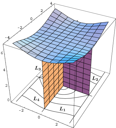
Figure 1: Decomposition in $N$

3.2 Auxiliary lemmas

Lemma 3.1.

Let $k\in(0,1)$, and let $p=p_{1}^{1}(k)$ be the root of equation $(\ref{f1=0})$. Then

$$p\in(0,p_{1}^{1})\quad\Rightarrow\quad f_{1}(p)>0,$$

$$p\in(p_{1}^{1},3K)\quad\Rightarrow\quad f_{1}(p)<0.$$

Proof.

The function $\displaystyle g_{1}(p)=\frac{f_{1}(p)}{\,{\operatorname{cn}\nolimits p}\,}$ is increasing at each interval $(K+2Kn,3K+2Kn)$, $n\in{\mathbb{Z}}$, since $\displaystyle\frac{\partial\,g_{1}}{\partial\,p}=\frac{\,{\operatorname{sn}\nolimits^{2}p}\,\,{\operatorname{dn}\nolimits^{2}p}\,}{\,{\operatorname{cn}\nolimits^{2}p}\,}\geq 0$. We have $\displaystyle g_{1}(p)=\frac{p^{3}}{3}+o(p^{3})$ as $p\to 0$, so $g_{1}(p)>0$ for $p\in(0,K)$, thus $f_{1}(p)>0$ for $p\in(0,p_{1}^{1})$. Further, the function $g_{1}(p)$ changes sign at $p_{1}^{1}$, thus $f_{1}(p)$ changes its sign at $p_{1}^{1}$ as well. ∎

Lemma 3.2.

The function $p=p_{1}^{1}(k)$, $k\in(0,1)$, defined by $(\ref{f1=0})$ satisfies the following properties:

• $p_{1}^{1}(k)$ is continuous on the interval $(0,1)$,

• $p_{1}^{1}(k)$ is smooth on the intervals $(0,k_{0})\cup(k_{0},1)$.

Proof.

Follows by the implicit function theorem. ∎

A plot of the function $p_{1}^{1}(k)$ is given in Fig. 3. Notice the vertical tangent at the point $(k,p)=(k_{0},2K(k_{0}))$, $k_{0}\approx 0.902$, and the vertical asymptote $k=1$.

Figure 2: Plot of the function $p_{1}^{1}(k)$

Figure 3: Plot of the function $\operatorname{am}\nolimits(p_{1}^{1}(k),k)$

Corollary 3.1.

The function $p_{1}\,:\,(0,1)\to(0,+\infty)$ given by $(\ref{p1(k)N1})$ is continuous.

Proof.

For $k\in[k_{0},1)$, the function $p_{1}(k)=p_{1}^{1}(k)$ is continuous by Lemma 3.2. And for $k\in(0,k_{0}]$, the function $p_{1}(k)=2K(k)$ is continuous as well. ∎

Lemma 3.3.

Consider sequences $k^{n}\in(0,1)$, $k^{n}\to 1-0$ and $p^{n}\in(0,K(k^{n}))$, $p^{n}\to+\infty$. Then $\operatorname{am}\nolimits(p^{n},k^{n})\to\pi/2$ as $n\to\infty$.

Here and below $\operatorname{am}\nolimits(p,k)$ is Jacobi’s amplitude [13].

Proof.

On any converging subsequence of the sequence $u^{n}=\operatorname{am}\nolimits(p^{n},k^{n})\in(0,\pi/2)$ we have $u^{n_{m}}\to\bar{u}\in[0,\pi/2]$. If $\bar{u}<\pi/2$, then $p^{n_{m}}=F(u^{n_{m}},k^{n_{m}})\to F(\bar{u},1)<+\infty$, a contradiction. ∎

Define the function $u_{1}^{1}(k)=\operatorname{am}\nolimits(p_{1}^{1}(k),k)$. By definition $(\ref{f1=0})$ and Propos. 11.6 [10], the function $u=u_{1}^{1}(k)$ is the first positive root of the equation

$$f_{u}(u,k)=\sin u\sqrt{1-k^{2}\sin^{2}u}-\cos u(2E(u,k)-F(u,k)),$$

moreover,

$$k\in(0,k_{0})\quad\Rightarrow\quad u_{1}^{1}\in(3\pi/2,\pi),$$

$$k=k_{0}\quad\Rightarrow\quad u_{1}^{1}=\pi,$$

$$k\in(k_{0},1)\quad\Rightarrow\quad u_{1}^{1}\in(\pi,\pi/2).$$

Lemma 3.4.

The function $u_{1}^{1}(k)$ satisfies the following properties:

• $u_{1}^{1}(k)$ decreases as $k\in(k_{0},1)$,

• $\lim_{k\to 1-0}u_{1}^{1}(k)=\pi/2$.

Proof.

(1) For $k\in(k_{0},1)$, $u\in(\pi/2,\pi)$ we have

$$\left.\frac{\partial\,f_{u}}{\partial\,u}\right|_{f_{u}=0}=\sqrt{1-k^{2}\sin^{2}u}\ \ \frac{\sin^{2}u}{\cos u}<0,$$

$$\left.\frac{\partial\,f_{u}}{\partial\,k}\right|_{f_{u}=0}=-\frac{\sqrt{1-k^{2}\sin^{2}u}\ \sin u-\cos u\ F(u,k)}{2k(1-k^{2})}<0,$$

thus

$$\frac{d\,u_{1}^{1}}{d\,k}=-\frac{\partial f_{u}/\partial k}{\partial f_{u}/\partial u}<0.$$

(2) The function $u_{1}^{1}(k)$ is decreasing for $k\in(k_{0},1)$, thus there exists a limit $\lim_{k\to 1-0}u_{1}^{1}(k)=\bar{u}\in[\pi/2,\pi)$. Assume by contradiction that $\bar{u}>\pi/2$. Then for any $\varepsilon>0$ the domain $\{(u,k)\in{\mathbb{R}}^{2}\mid u\in(\bar{u},\bar{u}+\varepsilon),\ k\in(1-\varepsilon,1)\}$ contains points such that $f_{u}(u,k)=0$. On the other hand, we have:

$$\lim_{(u,k)\to(\bar{u},1-0)}F(u,k)\geq\lim_{k\to 1-0}F(\pi/2,k)=+\infty,$$

$$\lim_{(u,k)\to(\bar{u},1-0)}f_{u}(u,k)=-\infty,$$

a contradiction. ∎

A plot of the function $u_{1}^{1}(k)$ is given in Fig. 3. Notice the vertical tangents at the points $(u,k)=(\pi,k_{0})$ and $(u,k)=(\pi/2,1)$.

Denote by $\overline{{\mathbb{R}}}$ the completed real line $[-\infty,+\infty]=\{-\infty\}\cup{\mathbb{R}}\cup\{+\infty\}$, with the basis of topology consisting of intervals $(a,b)$ and completed rays $[-\infty,b)$, $(a,+\infty]$ for $a,b\in{\mathbb{R}}$. In the following lemmas we consider a continuous function from a topological space to the topological space $\overline{{\mathbb{R}}}$.

Lemma 3.5.

The function $\mathbf{t}\,:\,N_{1}\cup N_{2}\cup N_{3}\to\overline{{\mathbb{R}}}$ given by $(\ref{tt})$–$(\ref{ttN3})$ is continuous.

Proof.

Notice first that the set

$$N_{1}\cup N_{2}\cup N_{3}=\{\lambda\in N\mid r>0,\ (\beta,c)\neq(0,0),\,(\pi,0)\}$$

is open.

If $\lambda\in N_{1}$, then the function $\mathbf{t}(\lambda)=2p_{1}(k)/\sqrt{r}$ is continuous by Cor. 3.1.

If $\lambda\in N_{2}$, then the function $\mathbf{t}(\lambda)=2kK(k)/\sqrt{r}$ is continuous as well.

Let $\lambda=(\varphi,k,r)\in N_{3}$, $k=1$, and let $\lambda_{n}\to\lambda$ as $n\to\infty$. We show that $\mathbf{t}(\lambda_{n})\to\mathbf{t}(\lambda)=+\infty$.

1) Let $\lambda_{n}=(\varphi_{n},k_{n},r_{n})\in N_{1}$ for all $n\in{\mathbb{N}}$. Then $k_{n}\to 1$, thus $K(k_{n})\to+\infty$, so $(K(k_{n}),2K(k_{n}))\ni p_{1}(k_{n})\to+\infty$; moreover, $r_{n}\to r$ as $n\to\infty$. Consequently, $\mathbf{t}(\lambda_{n})=2p_{1}(k_{n})/\sqrt{r_{n}}\to+\infty$.

2) Let $\lambda_{n}=(\varphi_{n},k_{n},r_{n})\in N_{2}$ for all $n\in{\mathbb{N}}$, then similarly $\mathbf{t}(\lambda_{n})=2k_{n}K(k_{n})/\sqrt{r_{n}}\to+\infty$.

3) Let $\lambda_{n}\in N_{3}$ for all $n\in{\mathbb{N}}$, then $\mathbf{t}(\lambda_{n})=+\infty\to+\infty$.

Thus for any sequence $\lambda_{n}\in N_{1}\cup N_{2}\cup N_{3}$ with $\lambda_{n}\to\lambda\in N_{3}$ we have $\mathbf{t}(\lambda_{n})\to+\infty$, so the function $\mathbf{t}$ is continuous on $N_{3}$. ∎

Define the following subset in the preimage of the exponential mapping:

$$K_{1}=\{\lambda=(\beta,c,r)\in N\mid\beta\in(0,\pi),\ c>0,\ r>0,\ \mathbf{t}(\lambda)>1\}.$$

Lemma 3.6.

The set $K_{1}$ is open.

Proof.

The set $K_{1}\subset N_{1}\cup N_{2}\cup N_{3}$ is determined by a system of strict inequalities for continuous functions, thus it is open (the function $\mathbf{t}(\lambda)$ is continuous by Lemma 3.5). ∎

3.3 Properties of decomposition in preimage
of exponential mapping

In this subsection we prove some topological properties of decomposition $(\ref{tNLi})$.

Lemma 3.7.

The set $L_{1}$ is open.

Proof.

Consider the vector field $\vec{P}=c\frac{\partial\,}{\partial\,\beta}-r\sin\beta\frac{\partial\,}{\partial\,c}\in\operatorname{Vec}\nolimits(N)$ determined by the equation of pendulum $(\ref{pend})$. We show that

$$L_{1}=e^{-1/2\vec{P}}(K_{1}),$$ (3.9)

where $e^{-1/2\vec{P}}\,:\,N\to N$ is the flow of the vector field $\vec{P}$ for the time $-1/2$.

Since energy $(\ref{E_r})$ is an integral of pendulum, then $\vec{P}E=0$, thus $e^{t\vec{P}}(N_{i})=N_{i}$, $i=1,2,3$. Further, the coordinates $(\varphi,p,k)$ rectify the flow of the vector field $\vec{P}$ (see $(\ref{rectify})$), so in these coordinates $\vec{P}=\frac{\partial\,}{\partial\,\varphi}$. Since

$$L_{1}\cap N_{1}=\{\lambda\in N_{1}\mid\varphi\in(-1/2,K/\sqrt{r}-1/2),\ p\in(0,p_{1}(k)),\ k\in(0,1)\},$$

$$K_{1}\cap N_{1}=\{\lambda\in N_{1}\mid\varphi\in(0,K/\sqrt{r}),\ p\in(0,p_{1}(k)),\ k\in(0,1)\},$$

it is obvious that $L_{1}\cap N_{1}=e^{-1/2\vec{P}}(K_{1}\cap N_{1})$.

Similarly it follows that $L_{1}\cap N_{i}=e^{-1/2\vec{P}}(K_{1}\cap N_{i})$ for $i=2,3$.

Then equality $(\ref{L1K1})$ follows. Since the set $K_{1}$ is open and the flow $e^{-1/2\vec{P}}\,:\,N\to N$ is a diffeomorphism, then the set $L_{1}$ is open as well. ∎

Lemma 3.8.

The set $L_{1}$ is arcwise connected.

Proof.

It is obvious from equalities $(\ref{L1N1})$–$(\ref{L1N3})$ that the sets $L_{1}\cap N_{i}$, $i=1,2,3$, are arcwise connected. Since any point in $L_{1}\cap N_{3}$ can be connected with some close points in $L_{1}\cap N_{1}$ and $L_{1}\cap N_{2}$ by a continuous curve, then the set $L_{1}$ is arcwise connected. ∎

In Sec. 9 [10] were defined discrete symmetries of the elastic problem — reflections $\varepsilon^{1}$, $\varepsilon^{2}$, $\varepsilon^{3}$ that act both in preimage and image of the exponential mapping, and commute with it.

Lemma 3.9.

• The mappings $\varepsilon^{i}\,:\,N\to N$, $i=1,2,3$, are diffeomorphisms.

• The reflections $\varepsilon^{i}$ permute the sets $L_{j}$ as shown by Table 2.

$$\begin{array}[]{|c|c|c|c|c|}\hline\cr L_{j}&L_{1}&L_{2}&L_{3}&L_{4}\\ \hline\cr\varepsilon^{1}(L_{j})&L_{2}&L_{1}&L_{4}&L_{3}\\ \hline\cr\varepsilon^{2}(L_{j})&L_{4}&L_{3}&L_{2}&L_{1}\\ \hline\cr\varepsilon^{3}(L_{j})&L_{3}&L_{4}&L_{1}&L_{2}\\ \hline\cr\end{array}$$

Table 2: Action of $\varepsilon^{i}$ on $L_{j}$

Proof.

(1) By the definition given in Subsec. 9.7 [10], we have $\varepsilon^{1}\,:\,(\beta,c,r)\mapsto(\beta_{1},-c_{1},r)$, where $e^{\vec{P}}(\beta,c,r)=(\beta_{1},c_{1},r)$. Since $e^{\vec{P}}$ is smooth, then $\varepsilon^{1}$ is smooth as well. Moreover, we have $\varepsilon^{1}\circ\varepsilon^{1}=\operatorname{Id}\nolimits$, thus $\varepsilon^{1}$ is a diffeomorphism. Similarly, $\varepsilon^{2}$ and $\varepsilon^{3}$ are diffeomorphisms.

(2) The reflection $\varepsilon^{1}$ preserves the coordinates $k$, $p$ and acts as follows on the coordinate $\tau$ of a point $\lambda=(p,\tau,k)\in N_{1}\cup N_{2}\cup N_{3}$:

$$\lambda\in N_{1}\quad\Rightarrow\quad\varepsilon^{1}\,:\,\tau\mapsto 2K-\tau,$$

$$\lambda\in N_{2}\cup N_{3}\quad\Rightarrow\quad\varepsilon^{1}\,:\,\tau\mapsto-\tau.$$

Thus $\varepsilon^{1}(L_{1}\cap N_{i})=L_{2}\cap N_{i}$, $i=1,2,3$. So $\varepsilon(L_{1})=L_{2}$.

Similarly one proves the remaining entries of Table 2. ∎

Proposition 3.1.

The sets $L_{i}$, $i=1,\dots,4$, are open and arcwise connected.

Proof.

Follows from Lemmas 3.7–3.9. ∎

3.4 Decomposition in image of exponential mapping

Recall that the time 1 attainable set of system $(\ref{sys1})$–$(\ref{sys3})$ is

$$\mathcal{A}=\{(x,y,\theta)\in M\mid x^{2}+y^{2}<1\text{ or }(x,y,\theta)=(1,0,0)\}.$$

Consider the following decomposition of this set:

$$\mathcal{A}=\widetilde{M}\sqcup M^{\prime},$$ (3.10)

$$\widetilde{M}=\{q\in\mathcal{A}\mid P(q)\sin(\theta/2)\neq 0\},$$

$$M^{\prime}=\{q\in\mathcal{A}\mid P(q)\sin(\theta/2)=0\},$$

$$M_{\pm}=\{q\in M\mid\theta\in(0,2\pi),\ x^{2}+y^{2}<1,\ \operatorname{sgn}\nolimits P(q)=\pm 1\},$$

$$\widetilde{M}=M_{+}\sqcup M_{-}.$$ (3.11)

The function $P(q)=x\sin(\theta/2)-y\cos(\theta/2)$ was introduced in [10], it is defined on $M$ up to sign. If $\theta\in(0,2\pi)$ as in $M_{\pm}$, then the function $P(q)$ is well-defined.

Decomposition $(\ref{tM+-})$ is shown in Fig. 4.

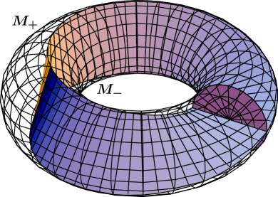
Figure 4: Decomposition in $M$

Lemma 3.10.

The sets $M_{+}$ and $M_{-}$ are open, arcwise connected, and simply connected.

Proof.

Obvious. ∎

Lemma 3.11.

The reflections $\varepsilon^{i}$ permute the sets $M_{\pm}$ as shown by Table 3.

$$\begin{array}[]{|c|c|c|}\hline\cr M_{\pm}&M_{+}&M_{-}\\ \hline\cr\varepsilon^{1}(M_{\pm})&M_{-}&M_{+}\\ \hline\cr\varepsilon^{2}(M_{\pm})&M_{-}&M_{+}\\ \hline\cr\varepsilon^{3}(M_{\pm})&M_{+}&M_{-}\\ \hline\cr\end{array}$$

Table 3: Action of $\varepsilon^{i}$ on $M_{\pm}$

Proof.

Action of reflections $\varepsilon^{i}$ in $M$ is given by formulas (9.10)–(9.12) [10], with appropriate choice of the branch of $\theta\in(0,2\pi)$:

$$\varepsilon^{1}\,:\,\left(\begin{array}[]{c}\theta\\ x\\ y\end{array}\right)\mapsto\left(\begin{array}[]{c}2\pi-\theta\\ x\cos\theta+y\sin\theta\\ -x\sin\theta+y\cos\theta\end{array}\right),$$ (3.18)

$$\varepsilon^{2}\,:\,\left(\begin{array}[]{c}\theta\\ x\\ y\end{array}\right)\mapsto\left(\begin{array}[]{c}\theta\\ x\cos\theta+y\sin\theta\\ x\sin\theta-y\cos\theta\end{array}\right),$$ (3.25)

$$\varepsilon^{3}\,:\,\left(\begin{array}[]{c}\theta\\ x\\ y\end{array}\right)\mapsto\left(\begin{array}[]{c}2\pi-\theta\\ x\\ -y\end{array}\right).$$ (3.32)

These formulas show that the reflections $\varepsilon^{i}$ preserve the restrictions $\theta\in(0,2\pi)$ and $x^{2}+y^{2}<1$, and imply the following transformation rules for the function $P$:

$$\varepsilon^{1}\,:\,P\mapsto-P,\qquad\varepsilon^{2}\,:\,P\mapsto-P,\qquad\varepsilon^{3}\,:\,P\mapsto P.$$

Then $\varepsilon^{1}(M_{\pm})=\varepsilon^{2}(M_{\pm})=M_{\mp}$ and $\varepsilon^{3}(M_{\pm})=M_{\pm}$, which gives Table 3. ∎

Lemma 3.12.

The mappings $\varepsilon^{i}\,:\,M\to M$, $i=1,2,3$, are diffeomorphisms.

Proof.

The reflections $\varepsilon^{i}$ are smooth by formulas (9.10)–(9.12) [10] and satisfy $\varepsilon^{i}\circ\varepsilon^{i}=\operatorname{Id}\nolimits$. ∎

Lemma 3.13.

The action of the exponential mapping on the sets $L_{i}$ is shown by Table 4.

$$\begin{array}[]{|c|c|c|c|c|}\hline\cr L_{i}&L_{1}&L_{2}&L_{3}&L_{4}\\ \hline\cr\operatorname{Exp}\nolimits(L_{i})&M_{+}&M_{-}&M_{+}&M_{-}\\ \hline\cr\end{array}$$

Table 4: Action of $\operatorname{Exp}\nolimits$ on $L_{i}$

Proof.

First we show that $\operatorname{Exp}\nolimits(L_{1})\subset M_{+}$.

Let $\lambda\in N_{1}$. It follows from the parameterisation of extremal trajectories obtained in [10] that

$$\sin\frac{\theta}{2}=\frac{2k\,{\operatorname{sn}\nolimits p}\,\,{\operatorname{dn}\nolimits p}\,\,{\operatorname{cn}\nolimits\tau}\,}{\Delta},\qquad\Delta=1-k^{2}\,{\operatorname{sn}\nolimits^{2}p}\,\,{\operatorname{sn}\nolimits^{2}\tau}\,,$$ (3.33)

$$P=\frac{4k\,{\operatorname{sn}\nolimits\tau}\,\,{\operatorname{dn}\nolimits\tau}\,f_{1}(p)}{\Delta}.$$ (3.34)

Let $\lambda\in L_{1}\cap N_{1}$. Then $\tau\in(0,K)$, thus $\,{\operatorname{sn}\nolimits\tau}\,>0$, $\,{\operatorname{dn}\nolimits\tau}\,>0$, $\,{\operatorname{cn}\nolimits\tau}\,>0$. Moreover, since $p\in(0,p_{1}(k))$, then $f_{1}(p)>0$ (see Lemma 3.1) and $\,{\operatorname{sn}\nolimits p}\,>0$, $\,{\operatorname{dn}\nolimits p}\,>0$. Thus $\sin\frac{\theta}{2}>0$, $P>0$, so $\operatorname{Exp}\nolimits(L_{1}\cap N_{1})\subset M_{+}$.

Let $\lambda\in N_{2}$. Then

$$\sin\frac{\theta}{2}=\frac{2\,{\operatorname{cn}\nolimits p}\,\,{\operatorname{sn}\nolimits p}\,\,{\operatorname{dn}\nolimits\tau}\,}{\Delta},$$ (3.35)

$$P=\frac{4k\,{\operatorname{sn}\nolimits\tau}\,\,{\operatorname{cn}\nolimits\tau}\,f_{2}(p)}{\sqrt{r}\Delta},$$ (3.36)

$$f_{2}(p)=(k^{2}\,{\operatorname{sn}\nolimits p}\,\,{\operatorname{cn}\nolimits p}\,+\,{\operatorname{dn}\nolimits p}\,((2-k^{2})p-2\operatorname{E}\nolimits(p)))/k.$$

Similarly to the case $\lambda\in L_{1}\cap N_{1}$, these formulas imply that $\operatorname{Exp}\nolimits(L_{1}\cap N_{2})\subset M_{+}$.

If $\lambda\in N_{3}$, then formulas $(\ref{sinth2N2})$, $(\ref{PN2})$ remain valid with $k=1$, and similarly to the case $\lambda\in L_{1}\cap N_{2}$ it follows that $\operatorname{Exp}\nolimits(L_{1}\cap N_{3})\subset M_{+}$.

Thus $\operatorname{Exp}\nolimits(L_{1})\subset M_{+}$.

We have $\varepsilon^{i}\circ\operatorname{Exp}\nolimits=\operatorname{Exp}\nolimits\circ\varepsilon^{i}$ on $N$ (see Propos. 9.2 [10]). Then by virtue of Lemmas 3.9 and 3.11 we get

$$\operatorname{Exp}\nolimits(L_{2})=\operatorname{Exp}\nolimits\circ\varepsilon^{1}(L_{1})=\varepsilon^{1}\circ\operatorname{Exp}\nolimits(L_{1})\subset\varepsilon^{1}(M_{+})=M_{-}.$$

Similarly it follows that $\operatorname{Exp}\nolimits(L_{3})\subset M_{+}$, $\operatorname{Exp}\nolimits(L_{4})\subset M_{-}$. ∎

4 Diffeomorphic properties
of exponential mapping

In this section we prove the main result of this work.

Theorem 4.1.

The following mappings are diffeomorphisms:

$$\operatorname{Exp}\nolimits\,:\,L_{1}\to M_{+},\quad\operatorname{Exp}\nolimits\,:\,L_{2}\to M_{+},\quad\operatorname{Exp}\nolimits\,:\,L_{3}\to M_{+},\quad\operatorname{Exp}\nolimits\,:\,L_{4}\to M_{-}.$$

By virtue of Lemmas 3.9, 3.12, 3.11, it is enough to prove the following statement.

Proposition 4.1.

The mapping $\operatorname{Exp}\nolimits\,:\,L_{1}\to M_{+}$ is a diffeomorphism.

We prove this statement by applying the following Hadamard’s global inverse function theorem.

Theorem 4.2 (Th. 6.2.8 [6]).

Let $X$, $Y$ be smooth manifolds and let $F\,:\,X\to Y$ be a smooth mapping such that:

1. $\dim X=\dim Y$,

2. $X$ and $Y$ are arcwise connected,

3. $Y$ is simply connected,

4. $F$ is nondegenerate,

5. $F$ is proper (i.e., preimage of a compact is a compact).

Then $F$ is a diffeomorphism.

Now we check hypotheses 4 and 5 of Th. 4.2 for the mapping $\operatorname{Exp}\nolimits\,:\,L_{1}\to M_{+}$.

Proposition 4.2.

The mapping $\operatorname{Exp}\nolimits\,:\,L_{1}\to M_{+}$ is nondegenerate.

Proof.

Theorem 5.1 [11] gives the following lower bound on the first conjugate time $t_{1}^{\operatorname{conj}}(\lambda)$ along extremal trajectory $\operatorname{Exp}\nolimits_{t}(\lambda)$:

$$\forall\lambda\in N\qquad t_{1}^{\operatorname{conj}}(\lambda)\geq\mathbf{t}(\lambda).$$

Let $\lambda\in L_{1}$, then $\mathbf{t}(\lambda)>1$, thus $t_{1}^{\operatorname{conj}}(\lambda)>1$. This means that the differential $\operatorname{Exp}\nolimits_{*\lambda}\,:\,T_{\lambda}N\to T_{q}M$, $q=\operatorname{Exp}\nolimits(\lambda)$, is nondegenerate. ∎

Proposition 4.3.

The mapping $\operatorname{Exp}\nolimits\,:\,L_{1}\to M_{+}$ is proper.

Proof.

Let $K\subset M_{+}$ be a compact. Denote the function $R(q)=x^{2}+y^{2}-1$. There exists $\varepsilon>0$ such that for any $q\in K$

$$\sin\frac{\theta}{2}\geq\varepsilon,\qquad P(q)\geq\varepsilon,\qquad-\varepsilon\geq R(q)\geq-1.$$ (4.1)

We prove that the preimage $S=\operatorname{Exp}\nolimits^{-1}(K)\subset L_{1}$ is compact, i.e., bounded and closed.

By contradiction, suppose first that $S$ is unbounded, then it contains a sequence $\lambda^{n}=(\tau^{n},p^{n},k^{n})\to\infty$.

If $k^{n}$ is separated from 1, then the sequences $\tau^{n}\in(0,K(k^{n}))$ and $p^{n}\in(0,2K(k^{n}))$ are bounded, thus $\lambda^{n}$ is bounded, a contradiction. Thus $k^{n}\to 1$ on a subsequence of $\lambda^{n}$ (we keep the notation $\lambda^{n}$ for this subsequence). Then $(\tau^{n},p^{n})\to\infty$.

1) Let $\lambda^{n}\in N_{1}$ for all $n\in{\mathbb{N}}$. Then we have decompositions $(\ref{sinth2N1})$, $(\ref{PN1})$ and obtain from parameterisation of extremal trajectories [10]

$$R=\frac{16\operatorname{E}\nolimits(p)(\operatorname{E}\nolimits(p)-p)}{r}+\frac{16k^{2}\,{\operatorname{sn}\nolimits p}\,\,{\operatorname{dn}\nolimits p}\,f_{1}(p)\,{\operatorname{sn}\nolimits^{2}\tau}\,}{r\Delta}.$$ (4.2)

1.1) Let $\tau^{n}\to\bar{\tau}\in[0,+\infty)$, $p^{n}\to\infty$, $k^{n}\to 1$. By Lemmas 3.3, 3.4, we have $\operatorname{am}\nolimits(p^{n},k^{n})\to\pi/2$, thus $\operatorname{sn}\nolimits(p^{n})\to 0$, $\operatorname{sn}\nolimits(\tau^{n})\to\operatorname{sn}\nolimits(\bar{\tau},1)=\tanh\bar{\tau}<1$, $\Delta\to 1-\tanh^{2}\bar{t}>0$, $\operatorname{dn}\nolimits(p^{n},k^{n})\to 1$. By virtue of $(\ref{sinth2N1})$, we have $\sin(\theta^{n}/2)\to 0$, which contradicts $(\ref{sinthPR})$.

1.2) The case $\tau^{n}\to+\infty$, $p^{n}\to\bar{p}\in[0,\infty)$ is considered similarly to the case 1.1).

1.3) Let $\tau^{n}\to+\infty$, $p^{n}\to+\infty$, $k^{n}\to 1$. Then $\operatorname{am}\nolimits(\tau^{n},k^{n})\to\pi/2$, $\operatorname{am}\nolimits(p^{n},k^{n})\to\pi/2$ by Lemmas 3.3, 3.4.

We have $\operatorname{E}\nolimits(p)=\operatorname{E}\nolimits(p^{n},k^{n})=E(\operatorname{am}\nolimits(p^{n},k^{n}),k^{n})\to E(\pi/2,1)=1$, thus
$\displaystyle\frac{\operatorname{E}\nolimits(p)(p-\operatorname{E}\nolimits(p))}{4p^{2}}\to 0$. By virtue of the inequalities $(\ref{sinthPR})$ for $R$, there exists a subsequence $\lambda^{n}$ on which $R(q^{n})\to-\varepsilon_{1}\leq-\varepsilon$. Then the second term in $(\ref{RN1})$ tends to $-\varepsilon_{1}<0$, which is impossible since this term is positive.

So the set $S\cap N_{1}$ does not contain sequences $\lambda^{n}\to\infty$, i.e., it is bounded.

2) Similarly it follows that the sets $S\cap N_{2}^{+}$ and $S\cap N_{3}^{+}$ are bounded. Thus the set $S\cap N_{2}^{+}$ is bounded.

3) The sets $S\cap N_{1}$, $S\cap N_{2}^{+}$, $S\cap N_{3}^{+}$ are bounded, thus $S$ is bounded as well.

Now we prove that $S$ is closed. Let $\lambda^{n}\in S$, $\lambda^{n}=(p^{n},\tau^{n},k^{n})\to(\bar{p},\bar{\tau},\bar{k})=\bar{\lambda}\in\operatorname{cl}\nolimits(L_{1})$. We show that $\bar{\lambda}\in S$.

1) Let $\lambda^{n}\in S\cap N_{1}$.

1.1) If $\bar{\lambda}\in L_{1}$, then $\bar{q}=\operatorname{Exp}\nolimits(\bar{\lambda})\in M_{+}$, on a subsequence $\operatorname{Exp}\nolimits(\lambda^{n})\to\bar{q}$, thus $\bar{q}\in K$ and $\bar{\lambda}\in S$.

1.2) Let $\bar{\lambda}\notin L_{1}$, thus

$$\bar{k}=0\quad\vee\quad\bar{k}=1\quad\vee\quad\bar{\tau}=0\quad\vee\quad\bar{\tau}=K\quad\vee\quad\bar{p}=0\quad\vee\quad\bar{p}=p_{1}.$$ (4.3)

Each of these conditions leads to a contradiction with inequalities $(\ref{sinthPR})$. For example, let $\bar{k}=0$. Then $k^{n}\to 0$, $p^{n}\to\bar{p}$, $\tau^{n}\to\bar{\tau}$, thus $\Delta\to 1$. By $(\ref{sinth2N1})$, $\sin(\theta/2)\to 0$, which contradicts $(\ref{sinthPR})$. All other cases in $(\ref{kbar=0})$ are considered similarly. Thus $\bar{\lambda}\in S$ in the case $\lambda^{n}\in S\cap N_{1}$.

2) Similarly, the inclusion $\bar{\lambda}\in S$ follows in the cases $\lambda^{n}\in S\cap N_{2}$ and $\lambda^{n}\in S\cap N_{3}$.

We proved that the set $S$ is closed. Since it is bounded as well, it is compact. Thus the mapping $\operatorname{Exp}\nolimits\,:\,L_{1}\to M_{+}$ is proper. ∎

Now we can prove Proposition 4.1.

Proof.

We check hypotheses of Th. 4.2 for the mapping $\operatorname{Exp}\nolimits\,:\,L_{1}\to M_{+}$. The sets $L_{1}$ and $M_{+}$ are open subsets in a 3-dimensional linear space (Lemmas 3.7 and 3.10). Moreover, we have:

1. $\dim L_{1}=\dim M_{+}=3$,

2. $L_{1}$ and $M_{+}$ are arcwise connected (Lemmas 3.8 and 3.10),

3. $M_{+}$ is simply connected (Lemma 3.10),

4. the mapping $\operatorname{Exp}\nolimits\,:\,L_{1}\to M_{+}$ is nondegenerate (Propos. 4.2),

5. the mapping $\operatorname{Exp}\nolimits\,:\,L_{1}\to M_{+}$ is proper (Propos. 4.3).

By Theorem 4.2, the mapping $\operatorname{Exp}\nolimits\,:\,L_{1}\to M_{+}$ is a diffeomorphism. ∎

By virtue of Lemmas 3.9, 3.12, 3.11, Theorem 4.1 follows. This theorem implies that

$$\operatorname{Exp}\nolimits(\widetilde{N})=\widetilde{M}.$$ (4.4)

5 Action of exponential mapping
on the boundary of diffeomorphic domains

Define the following subsets in the boundary of the set $\widetilde{M}$:

$$M_{P}=\{q\in\mathcal{A}\mid P(q)=0\},$$

$$M_{\theta}=\{q\in\mathcal{A}\mid\sin(\theta/2)=0\},$$

$$V=\{(x,y,\theta)=(1,0,0)\}.$$

Proposition 5.1.

We have

$$\operatorname{Exp}\nolimits(N^{\prime})=M^{\prime}.$$ (5.1)

Proof.

Recall decomposition $(\ref{N'})$ of the set $N^{\prime}$.

It follows from definitions $(\ref{N4})$–$(\ref{N7})$ and the parameterisation of extremal trajectories [10] that

$$\operatorname{Exp}\nolimits(N_{4})=\operatorname{Exp}\nolimits(N_{5})=\operatorname{Exp}\nolimits(N_{7})=V,$$ (5.2)

$$\operatorname{Exp}\nolimits(\widehat{N}_{6})\subset M_{P}\subset M^{\prime}.$$ (5.3)

Further, it follows from formulas $(\ref{sinth2N1})$–$(\ref{PN2})$ that

$$\operatorname{Exp}\nolimits(N_{1-3}^{\prime})\subset M_{\theta}\cup M_{P}\subset M^{\prime}.$$ (5.4)

Then we obtain from $(\ref{ExpN457})$–$(\ref{ExpMthMPM'})$ that $\operatorname{Exp}\nolimits(N^{\prime})\subset M^{\prime}$. But the mapping $\operatorname{Exp}\nolimits\,:\,\widehat{N}\to\mathcal{A}$ is surjective, then equalities $(\ref{NhatNtilde})$, $(\ref{AMtilde})$, $(\ref{ExpNtildeMtilde})$ imply equality $(\ref{ExpN'M'})$. ∎

6 Optimal elasticae
for various boundary conditions

In this section we describe optimal trajectories for various terminal points $q_{1}=(x_{1},y_{1},\theta_{1})\in\mathcal{A}$.

6.1 Generic boundary conditions

let $q_{1}\in M_{+}$, then by Th. 4.1 there exist a unique $\lambda_{1}\in L_{1}$ and a unique $\lambda_{3}\in L_{3}$ such that $\operatorname{Exp}\nolimits(\lambda_{1})=\operatorname{Exp}\nolimits(\lambda_{3})=q_{1}$. Since $\operatorname{Exp}\nolimits(L_{2})=\operatorname{Exp}\nolimits(L_{4})=M_{-}$ and $\operatorname{Exp}\nolimits(N^{\prime})=M^{\prime}$, the equation

$$\operatorname{Exp}\nolimits(\lambda)=q_{1},\qquad\lambda\in\widehat{N},$$ (6.1)

has only two solutions, $\lambda_{1}$ and $\lambda_{3}$. By virtue of existence of optimal trajectory connecting $q_{0}$ to $q_{1}$, it should be $q^{1}(t)=\operatorname{Exp}\nolimits_{t}(\lambda_{1})$ or $q^{3}(t)=\operatorname{Exp}\nolimits_{t}(\lambda_{3})$. In order to find the optimal trajectory, one should compare the costs $J[q^{i}]=\frac{1}{2}\int_{0}^{1}(c_{t}^{i})^{2}\,dt$, $i=1,3$, of the competing candidates $q^{1}(t)$ and $q^{3}(t)$ and choose the less one, see Fig. 5.

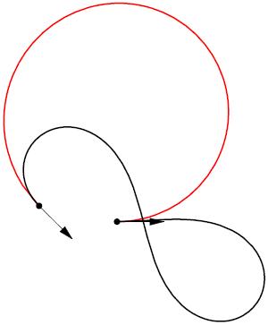
Figure 5: Competing elasticae with the same boundary conditions

If $J[q^{1}]\neq J[q^{3}]$, then the optimal trajectory is unique.

If $J[q^{1}]=J[q^{3}]$, then there are two optimal trajectories coming to the point $q_{1}$. (See example of the corresponding elasticae at Fig. 6). Such points $q_{1}$ are Maxwell points that arise due to some unclear reason different from the reflections $\varepsilon^{i}$.

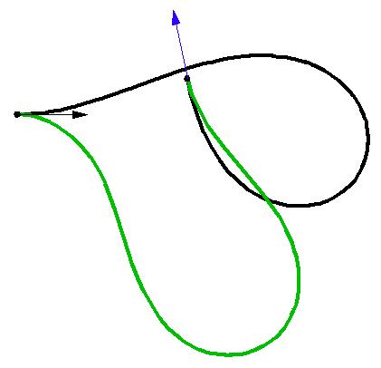
Figure 6: Two optimal non-symmetric elasticae with the same boundary conditions

If $q_{1}\in M_{-}$, then the analysis of optimal trajectories is similar to the case $q_{1}\in M_{+}$.

A. Ardentov designed a software in Mathematica [14] for numerical computation of optimal elasticae for $q_{1}\in\widetilde{M}$ by solving the equation $(\ref{Explamq1})$, the software and algorithm are described in [4]. An example of a sequence of optimal elasticae computed by this software for a given sequence of boundary conditions is given in Fig. 7.

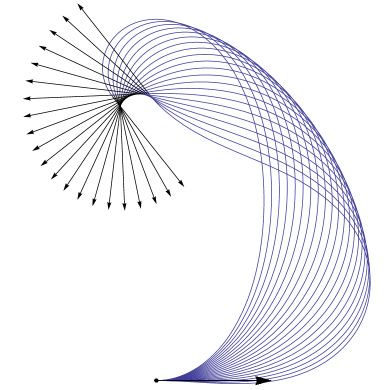
Figure 7: Sequence of optimal elasticae

6.2 The case $y_{1}=0$, $\theta_{1}=\pi$

6.2.1 The case $x_{1}>0$

We have $P(q_{1})=x_{1}>0$, thus $q_{1}\in M_{+}$. As shown in Subsec. 6.1, the equation $(\ref{Explamq1})$ has solutions $\lambda_{1}\in L_{1}$ and $\lambda_{3}\in L_{3}$. By $(\ref{eps3txy})$, $\varepsilon^{3}(q_{1})=q_{1}$, thus $\varepsilon^{3}(\lambda_{1})=\lambda_{3}$. Then the trajectories $q_{1}(t)=\operatorname{Exp}\nolimits_{t}(\lambda_{1})$ and $q_{3}(t)=\operatorname{Exp}\nolimits_{t}(\lambda_{3})$ have the same cost, thus they are both optimal. The corresponding optimal inflectional elasticae are symmetric w.r.t. the line $y=0$, see Fig. 9.

6.2.2 The case $x_{1}<0$

This case is similar to the case $x_{1}>0$, see Fig. 9.

6.2.3 The case $x_{1}=0$

It follows from results of Secs. 11.6–11.10 [10] that in the case $(x_{1},y_{1},\theta_{1})=(0,0,\pi)$ the equation $(\ref{Explamq1})$ has solutions $\lambda=(p,\tau,k)\in N_{1}$ with $\,{\operatorname{sn}\nolimits\tau}\,=0$, $1-2k^{2}\,{\operatorname{sn}\nolimits^{2}p}\,=0$, $2\operatorname{E}\nolimits(p)-p=0$. Then there exists a unique optimal elastica shown in Fig. 10.

Figure 8: Optimal elasticae for $(x_{1},y_{1},\theta_{1})=(x_{1},0,\pi)$, $x_{1}>0$

Figure 9: Optimal elasticae for $(x_{1},y_{1},\theta_{1})=(x_{1},0,0)$, $x_{1}<0$

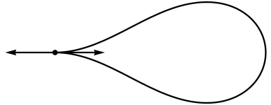
Figure 10: Optimal elastica for $(x_{1},y_{1},\theta_{1})=(0,0,\pi)$

6.3 The case $y_{1}=\theta_{1}=0$

6.3.1 The case $x_{1}=0$

This case was studied in [12], it was shown that there exist two optimal elasticae — circles symmetric w.r.t. the line $y=0$.

6.3.2 The case $x_{1}\neq 0$

One can show that in the case $x_{1}>0$ there are two or four optimal elasticae: there exists $x_{*}\in(0.4,0.5)$ such that

• if $x_{1}\in(0,x_{*})$, then there are two optimal non-inflectional elasticae, see Fig. 12,

• if $x_{1}=x_{*}$, then there are four optimal elasticae (two inflectional and two non-inflectional ones), see Fig. 13,

• if $x_{1}\in(x_{*},1)$, then there are two optimal inflectional elasticae, see Fig. 12.

Figure 11: Optimal elasticae for $(x_{1},y_{1},\theta_{1})=(x_{1},0,0)$, $0<x_{1}<x_{*}$

Figure 12: Optimal elasticae for $(x_{1},y_{1},\theta_{1})=(x_{1},0,0)$, $x_{*}<x_{1}<1$

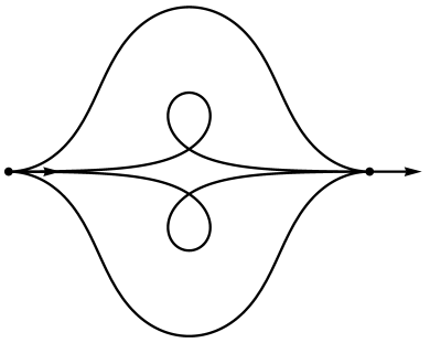
Figure 13: Optimal elasticae for $(x_{1},y_{1},\theta_{1})=(x_{*},0,0)$

In the case $x_{1}<0$ there are two optimal non-inflectional elasticae, see Fig. 14.

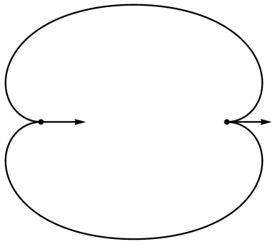
Figure 14: Optimal elasticae for $(x_{1},y_{1},\theta_{1})=(x_{1},0,0)$, $x_{1}<0$

6.4 The case $x_{1}=1$, $y_{1}=0$, $\theta_{1}=0$

In this case there exists a unique optimal elastica — the straight line.

7 Conclusion

This paper completes our planned study of Euler’s elastic problem via geometric control techniques [2]. The theoretical analysis describes the structure of optimal solutions and yields effective computation algorithms for numerical evaluation of these solutions for given boundary conditions. We believe that the approach developed in the study of Euler’s problem would be useful for other symmetric optimal control problems, e.g. invariant sub-Riemannian problems on 3-D Lie groups [1], nilpotent sub-Riemannian problems [3, 9], problems on rolling sphere [8], and others.

References

- [1] Agrachev A.A., Barilari D.: Sub-Riemannian structures on 3D Lie groups, J. Dynam. Control Systems 18 (2012), No. 1, 21–44.
- [2] A.A. Agrachev, Yu. L. Sachkov, Geometric control theory, Fizmatlit, Moscow 2004; English transl. Control Theory from the Geometric Viewpoint, Springer-Verlag, Berlin 2004.
- [3] A..A. Ardentov, Yu.L. Sachkov, Extremal trajectories in nilpotent sub-Riemannian problem on Engel group, Sbornik Mathematics, 202 (2011), No. 11, 31–54. English translation: Sbornik: Mathematics (2011), 202(11):1593–1616.
- [4] A.A. Ardentov, Yu.L. Sachkov, Solution of Euler’s elastic problem, Avtomatika i Telemekhanika, 2009, No. 4, 78–88. (in Russian, English translation in Automation and remote control.)
- [5] L.Euler, Methodus inveniendi lineas curvas maximi minimive proprietate gaudentes, sive Solutio problematis isoperimitrici latissimo sensu accepti, Lausanne, Geneva, 1744.
- [6] S. G. Krantz, H. R. Parks, The Implicit Function Theorem: History, Theory, and Applications, Birkauser, 2001.
- [7] A.E.H.Love, A Treatise on the Mathematical Theory of Elasticity, 4th ed., New York: Dover, 1927.
- [8] A. Mashtakov, Yu.L. Sachkov, Extremal trajectories and Maxwell points in the plate-ball problem, Sbornik Mathematics, 202 (2011), No. 9, 97–120.
- [9] Yu. L. Sachkov, Complete description of the Maxwell strata in the generalized Dido problem (in Russian), Matem. Sbornik, 197 (2006), 6: 111–160. English translation in: Sbornik: Mathematics, 197 (2006), 6: 901–950.
- [10] Yu. L. Sachkov, Maxwell strata in the Euler elastic problem. J. Dynam. Control Systems 14 (2008), No. 2, 169–234.
- [11] Yu.Sachkov, Conjugate points in Euler’s elastic problem, Journal of Dynamical and Control Systems, 2008 Vol. 14 (2008), No. 3 (July), 409–439.
- [12] Yu. L. Sachkov, Closed Euler elasticae, Proceedings of the Steklov Institute of Mathematics, 2012, vol. 278, pp. 218-–232.
- [13] E.T. Whittaker, G.N. Watson, A Course of Modern Analysis. An introduction to the general theory of infinite processes and of analytic functions; with an account of principal transcendental functions, Cambridge University Press, Cambridge 1996.
- [14] S. Wolfram, Mathematica: a system for doing mathematics by computer, Addison-Wesley, Reading, MA 1991.