Enhancing community detection using a network weighting strategy

Abstract

A community within a network is a group of vertices densely connected to each other but less connected to the vertices outside. The problem of detecting communities in large networks plays a key role in a wide range of research areas, e.g. Computer Science, Biology and Sociology.

Most of the existing algorithms to find communities count on the topological features of the network and often do not scale well on large, real-life instances.

In this article we propose a strategy to enhance existing community detection algorithms by adding a pre-processing step in which edges are weighted according to their centrality w.r.t. the network topology. In our approach, the centrality of an edge reflects its contribute to making arbitrary graph tranversals, i.e., spreading messages over the network, as short as possible. Our strategy is able to effectively complements information about network topology and it can be used as an additional tool to enhance community detection. The computation of edge centralities is carried out by performing multiple random walks of bounded length on the network. Our method makes the computation of edge centralities feasible also on large-scale networks. It has been tested in conjunction with three state-of-the-art community detection algorithms, namely the Louvain method, COPRA and OSLOM. Experimental results show that our method raises the accuracy of existing algorithms both on synthetic and real-life datasets.

1 Introduction

Networks are a powerful tool to model real-life complex systems in many research fields like Biology, Sociology, Economy and Computer Science [15, 12]. Due to their dynamics and sheer size, networks representing online social networks, e.g., Facebook, are a fascinating, and challenging, example of network models.

Most networks representing real-life systems show the so-called community structure feature [18]: vertices tend to organize themselves in groups (called communities or clusters) such that the number of edges linking vertices of the same group is much higher than the number of edges joining vertices belonging to different groups.

The ability to detect a community within a larger network plays a key role in understanding how systems are organized: communities, in fact, can be regarded as modules whose functions or properties are, to some extent, separable from other modules. The detection of communities is instrumental in understanding what are the main modules composing a real-life system, how these modules interact and, finally, how they evolve and impact the overall network and its functions. Concrete examples from the biological domain rise from the task of understanding the functioning of metabolic networks [27], gene regulatory networks [26] or other forms of interactions among proteins [49].

In Computer Science and Sociology, community detection algorithms are a powerful tool to understand how humans interact. There are, in fact, many reasons prompting users to join communities or to form new ones: people may decide to join a community because they share some interests with other community members [7] or because their attributes (like class or race) or cultural interests match well with those of the members of an already established community [39]. Finally, the Sociology literature shows that other factors (like ideologies, and attitudes of the members of a community) can prompt a user to join a community [32]. Understanding the processes leading a user to join a community can, therefore, have a deep practical impact: for instance, in the design of advertisement and business applications, it is crucial to understand whether or not communities in a social network consist of persons sharing the same needs and tastes. If such an hypothesis holds true it is possible to selectively disseminate commercial advertisements only to its members (who might be interested in those ads) rather than to the whole audience of the social network.

Due to its relevance, community detection has attracted the interest of many researchers and several, often interdisciplinary, approaches have been proposed. Most of the existing community detection approaches aim at finding pairwise disjoint communities, i.e., communities that do not share members (represented by vertices of the network). However, in the latest years, some researchers started studying the problem of finding overlapping communities, i.e., a relaxed version where a given vertex may belong to multiple communities [44, 25, 36].

A major avenue to finding communities relies on the so-called spectral clustering techniques [43, 50, 29]. Spectral clustering aims at partitioning a graph into subsets of vertices, called cuts. The problem of finding the optimal cuts is formulated as an optimization problem. The main limitation of spectral clustering is that one has to know, or fix, in advance the number and the size of communities in the network. Hence, this strategy is unfeasible when the purpose is to discover the unknown community structure of a network.

A further and relevant research line coincides with the introduction of a function called network modularity (usually denoted as $Q$) to quantitatively assess how structured in communities a given network is [23, 6, 13]. In brief, the network modularity of a given network $\mathcal{N}$ is defined as the fraction of all edges that lie within communities minus the expected value of the same quantity in a random graph $\mathcal{N}^{{}^{\prime}}$ so that: i) it has the same number of vertices of $\mathcal{N}$, ii) each vertex of $\mathcal{N}^{{}^{\prime}}$ has the same degree of its peer in $\mathcal{N}$ and iii) edges are placed randomly with uniform probability.

The introduction of the network modularity allows to turn the problem of finding communities into an optimization problem whose goal is to find a partitioning of the network capable of maximizing $Q$. Unfortunately, the maximization of $Q$ is an NP-hard problem [5] thus heuristics are required to find solutions (even near-optimal) and, at the same time, to guarantee reasonable computational costs/scalability.

Existing approaches based on modularity maximization suffer, however, from two major drawbacks. The first drawback is that methods that are actually able to achieve high values for $Q$ work only on networks of small/medium size. Consider, for instance, the first (and one of the most popular) algorithm to maximize modularity: the Girvan-Newman algorithm [23, 42]. It iteratively removes edges, with the goal of partitioning the network into increasingly-disjoint communities. Edges to be removed are selected according to their betwenness centrality: a measure of fraction of shortest paths between vertices that traverse that particular edge. Which in turn is a computationally-heavy measure, as it depends directly on the number of vertices. Hence, Girvan-Newman and similar methods are computationally expensive and do not scale well to the size of real-life networks consisting of, at least, millions of vertices and edges. Indeed, methods explicitly designed to handle large networks are based on optimization techniques like simulated annealing [28] or extremal optimization [13] and, therefore, the solution they produce may be sub-optimal. The second drawback is the so-called resolution limit [19]: communities consisting of a number of vertices smaller than a threshold (which in turn depends on the number of edges of the network) are not detected because the optimization procedure combines – with the goal of maximizing Q – small groups of vertices into larger ones.

Several procedures have been proposed to alleviate the resolution limit problem such as providing novel definition of modularity [38] or adding weights to the edges [34, 2]. To sum it up, despite the recent advances, community detection is still an open problem, even more so when we consider the growth, in sheer size and complexity, of online social networks.

In this article we propose a novel strategy to finding communities in networks which is based on the idea of introducing a measure of edge centrality and weighting edges according to their centrality. Our ultimate goal, therefore, is meta-algorithmic: not to introduce yet another community detection algorithm but to develop a pre-processing step devoted to weight the edges of the network. Once the weights have been computed, existing community detection algorithms will execute with better results.

The basis of our approach to the definition of edge weights, is the observation that in real-life social networks, a community can be intuitively depicted as a group of participants (vertices) which frequently interact with each other (or at least more frequently than they do with third parties). For instance, studies on online social networks like Facebook [16, 17] or Twitter [21] have shown that individuals belonging to the same community tend to frequently exchange messages with each other and seldom with people residing out of the community itself. This implies the existence of preferential pathways along which information flows easily. Hence, social links can be ranked according to their capacity to facilitate the process of information propagation.

In fact, we believe that our approach represents a breakthrough because the methods considered until now rely only on the knowledge of the network topology whereas our approach suggests to complement information related to the network topology with information assessing the tendency of each edge to transfer information.

A parameter similar to our edge weighting was proposed by Fortunato et al. in [20] and is called efficiency. The efficiency of a pair of vertices i and j is defined as the inverse of the length of the shortest path(s) connecting i to j. The efficiency measure was used in the same paper to design a greedy algorithm to find communities; experimental results were carried out over real and artificial small networks to provide an evidence of the effectiveness of this parameter.

Unfortunately, efficiency can not be generalized to large-scale networks like Facebook. In fact, to compute shortest paths, the whole network topology should be inspected and such an assumption does not hold true in real social networks. In any case, computing shortest paths in networks is costly, thus the computation of the network efficiency could be unfeasible over large networks.

Our approach is tailored to large networks and addresses those issues by means of the random walks technique to simulate message passing. Random walks have been successfully exploited to simulate message passing in networks with the goal of computing node centrality [41] and, in this article, we propose to extend them to the computation of edge weights.

We execute multiple random walks and assign to edges a weight that is equal to the cumulative frequency of selecting that edge in a simulated random walk. This choice is in keep with our previous considerations because, in our procedure, an edge has a high rank if it is frequently selected, i.e., if it is frequently exploited to convey messages. In addition, paths generated in our simulations have to satisfy two further requirements: (i) an edge can be selected only once in a random walk in order to avoid that the weight of an edge may be excessively inflated, and (ii) the random walks consist of up to $\kappa$ edges, $\kappa$ being a fixed integer. In such a way, we acknowledge Friedkin’s postulate [22] that the more distant two vertices, the less they influence each other. Moreover, the message propagation process is intended as a finite-steps process instead of a infinite one, which is reasonable in the context of real-life and online social networks where the spread of a given information sooner or later stops. The weight associated with each edge according to this strategy is called $\kappa$-path edge centrality. Its accuracy as an estimate of an edge’s importance depends, of course, on several factors, including the number of random walks attempted and possible biases. To the best of our knowledge, there are only two previous works concerning edge weighting in community detection, i.e., [34] and [2]. In those approaches the weight of a target edge is determined by computing some global network metrics like edge betwenness [34] or by considering cycles of fixed length k that include the target edge [2]. Inevitably, those approaches may not scale up well. Our approach differs from those previous works since it exploits random walks to compute edge weights and, therefore, it does not require to know in advance the whole network topology.

To sum it up, these are the main contributions of this article:

• We provide a formal definition of $\kappa$-path edge centrality and describe an approximate algorithm called WERW-Kpath (Weighted Edge Random Walk - $\kappa$ Path) to efficiently compute the $\kappa$-path edge centrality.

• We prove that our WERW-Kpath algorithm can approximate the actual value of centrality of an arbitrary edge with an error less than $\frac{1}{|E|}$, $|E|$ being the number of edges in the network, by performing $O(\kappa|E|)$ iterations. The WERW-Kpath algorithm is fast because its computational complexity is nearly-linear in the number of edges of the network but, at the same time, it yields precise results.

• We show how our edge weighting procedure can be combined with three existing, state-of-the-art algorithms for community detection, namely the Louvain method [3, 11], COPRA [25] and OSLOM [36].

• We report on the experimental assessment of our approach on both real and artificial network datasets. In particular, we considered 9 real-world network datasets and the largest, a sample from Facebook, consists of 613,497 vertices and 2,045,030 edges. Experiments on those networks show that combining WERW-Kpath with the algorithms mentioned above leads to an increase of network modularity up to 16%.

  Regarding the artificial networks, the experimental validation was conducted as follows: first, 72 artificial networks were generated, by exploiting the LFR benchmark [35]; in this way, we managed networks whose community structure was known in advance. Then, we compared communities found by our approach in conjunction with the three methods above by using the so-called Normalized Mutual Information measure from Information Theory. Experiments on these networks showed that our approach is able to alleviate the resolution limit problem. To make our research results reproducible, the prototype we implemented is freely available for download.

This article is organized as follows: in Section 2 we review existing approaches to finding communities in networks, whereas in Section 3 we describe in detail our approach. In Section 4 we discuss the WERW-Kpath algorithm; Section 5 describes our proposal of adopting the WERW-KPath algorithm in conjunction with community detection algorithms to enhance their performance. Section 6 is devoted to illustrate the experiments we carried out and to discuss the results. Section 7 covers some related literature and, finally, in Section 8, we draw our conclusions and discuss possible developments.

2 Background

Recently, a huge amount of research work has concerned the detection of community structures inside networks. In this section we describe some of the existing approaches to detecting communities; here and throughout this article we will use the terms network and graph interchangeably. Of course, the material presented in this section cannot be exhaustive and we refer the reader to comprehensive surveys like [45, 18].

Given a network represented by a graph $G=\langle V,E\rangle$, the community structure is a partition $P=\{C_{1},C_{2},\ldots,C_{r}\}$ of the vertices of $G$ such that, for each $C_{i}\in P$, the number of edges linking vertices in $C_{i}$ is high in comparison to the number of edges linking vertices on two distinct sets. Each set $C_{i}$ is called community.

Today, the most popular techniques to find communities are: (i) spectral clustering, and, (ii) network modularity maximization. In the following we shall discuss approaches belonging to each of these categories in detail.

2.1 Spectral Clustering techniques

Spectral Clustering techniques rely on the idea of partitioning a graph into subsets of vertices, called cuts. The number of cuts to be generated is fixed in such a way as to minimize a given objective function.

The maximization of this objective function, however, has been proved to be NP-hard. Therefore, different approximate techniques have been proposed. For instance, in [43], the authors suggest to use the Laplacian matrix $L$ of a graph $G$. We recall that the Laplacian matrix $L$ of $G=\langle V,E\rangle$ is a $|V|\times|V|$ matrix such that $L_{ij}=k_{i}\delta(i,j)-A_{ij}$, where $k_{i}$ is the degree of a vertex $i$, $\delta(i,j)$ is the Kronecker symbol (that is, $\delta(i,j)=1$ if and only if $i=j$ and 0 otherwise) and $A_{ij}$ is the adjacency matrix of $G$. Authors in [43] propose to compute the top-$k$ eigenvectors of $L$, i.e., the eigenvector of $L$ associated with the $k$ eigenvalues having the largest magnitude. The space of objects to cluster (source space) is then mapped onto the space generated by these eigenvectors (target space). Finally, the k-means clustering algorithm [30] is applied on the points in the target space (with $k$ dimensions).

Another approach relies on the strategy of ratio cut partitioning [50, 29]. This is a function that, if minimized, allows the identification of large clusters with a minimum number of outgoing interconnections. More recently, some authors [40] rely on the spectral decomposition of sparse matrices to find communities.

The main issue with spectral clustering techniques is that one has to know in advance the number and the size of communities comprised in the given network. This makes this strategy unfeasible if the purpose is to unveil the community structure of a network. Finally, Shah et al. [47] proved that this strategy could not work well if the given network contains densely-connected yet small-sized communities.

2.2 Network Modularity Maximization

Strategies based on network modularity define a measure, called modularity and usually denoted as Q, to assess the quality of a partitioning of a graph $G$ and aim at finding the partition of G that maximizes Q. Approaches based on network modularity rely on the idea that random graphs are not expected to exhibit a community structure. Therefore, given a graph $G$ and a subgraph $C\subseteq G$, the null model $G^{\prime}$ associated with $G$ is defined as a graph having the same number of vertices of $G$ and obtained by preserving some of the structural properties of $G$. For instance, $G^{\prime}$ could have the same number of edges of $G$ but these edges could be placed with a uniform probability among all pairs of nodes; in such a case $G^{\prime}$ is an example of a Bernoulli random graph [18].

Thanks to the null model, it is possible to decide whether a subgraph $C\subseteq G$ is a cluster or not. In fact, since $G$ and $G^{\prime}$ have the same vertices, we can consider the subgraph $C^{\prime}\subseteq G^{\prime}$ obtained by isolating, in $G^{\prime}$, the vertices forming $C$ in $G$. As claimed before, the null model is expected to exibit no community structure and, therefore, we expect that $C^{\prime}$ is not a community. Therefore, if the density of internal edges of $C$ is higher than that of $C^{\prime}$, we can conclude that $C$ is a community.

Accordingly, the network modularity function is defined as follows

$$Q=\frac{1}{2m}\sum_{i,j}\left(A_{ij}-P_{ij}\right)\delta(C_{i},C_{j}).$$

Here $m$ is the total number of edges in $G$, $A_{ij}$ is the adjacency matrix of $G$ (i.e., $A_{ij}=1$ if there is an edge from $i$ to $j$ and 0 otherwise, $P_{ij}$ is the expected number of edges between $i$ and $j$ in the null model. As usual, $\delta(\cdot,\cdot)$ is the Kronecker symbol.

Various null models are, in principle, allowed and, for each of them, we could derive a suitable expression for $P_{ij}$. The most common choice, however, is to assume that $P_{ij}$ is proportional to the product of the degrees $k_{i}$ and $k_{j}$ of $i$ and $j$ respectively. According to this choice, $Q$ can be rewritten as follows

$$Q=\frac{1}{2m}\sum_{i,j}\left(A_{ij}-\frac{k_{i}\cdot k_{j}}{2m}\right)\delta(C_{i},C_{j})$$ (1)

Equation 1 can be simplified by observing that only vertices belonging to the same community provide a non-zero contribution to the sum. In fact, if $i$ and $j$ would belong to different communities then $C_{i}\neq C_{j}$ and $\delta(C_{i},C_{j})=0$ by definition. As a result, we can rewrite the modularity function $Q$ as follows

$$Q=\sum_{c=1}^{n_{c}}\left[\frac{l_{c}}{m}-\left(\frac{d_{c}}{2m}\right)^{2}\right]$$ (2)

where $n_{c}$ is the number of communities, $l_{c}$ is the total number of edges joining vertices inside the community $c$ and $d_{c}$ is the sum of the degrees of the vertices composing $c$. In Equation (2), for a fixed community $c$, the first term, i.e., $\frac{l_{c}}{m}$ (called coverage) is the fraction of the edges of the graph inside $c$, whereas the second term $\left(\frac{d_{c}}{2m}\right)^{2}$ is the expected fraction of edges that would belong to $c$ in a random graph with the same degree distribution of $G$.

The problem of maximizing $Q$ has been proved to be NP-hard [5]. To this purpose, several heuristic strategies to maximize the network modularity $Q$ have been proposed as to date. Probably, the most popular one is known as the Girvan-Newman strategy [23, 42].

In this approach, edges are ranked by using a parameter known as edge betweenness centrality. The edge betweenness centrality $B(e)$ of a given edge $e\in E$ is defined as

$$B(e)=\sum_{v_{i}\in V}\sum_{v_{l}\in V}\frac{np_{e}(v_{i},v_{l})}{np(v_{i},v_{l})}$$ (3)

where $v_{i}$ and $v_{l}$ are vertices in $V$, $np(v_{i},v_{l})$ is the number of shortest paths connecting $v_{i}$ and $v_{l}$ and $np_{e}(v_{i},v_{l})$ is the number of the shortest paths between $v_{i}$ and $v_{l}$ containing $e$.

Given the definition of edge betweenness centrality, it is possible to maximize the network modularity by progressively deleting edges with the highest value of betweenness centrality, based on the consideration that they shall connect vertices belonging to different communities [42]. The process iterates until a significant increase of $Q$ is obtained. At each iteration, each connected component of $G$ identifies a community. Unfortunately, the computational cost of this strategy is $O(|V|^{3})$ and this makes it unsuitable for the analysis of large networks. The most time-expensive part of the Girvan-Newman strategy is the calculation of the betweenness centrality. Efficient algorithms have been designed to approximate the edge betweenness [4]; for real-life networks the computational costs still remains prohibitive, unfortunately.

Several variants of this strategy have been proposed during the years, such as the Fast Clustering Algorithm provided by Clauset, Newman and Moore [6], that runs in $O(|V|\log|V|)$ on sparse graphs. In [13], Duch and Arenas proposed the extremal optimization method based on a fast agglomerative approach whose worst-case time complexity is $O(|V|^{2}\log|V|)$.

An interesting network modularity maximization strategy is provided in the so-called Louvain method (LM) [3, 11]. LM has been tested in our experimental trials in conjunction with our approach to weighting edges; we present a detailed description of it in Section 5.

The approaches mentioned above use greedy strategies to maximize $Q$. In [27] the authors propose to use simulated annealing to maximize $Q$. This approach achieves a high accuracy but can as well be computationally very expensive. In general terms, the advantage of simulated annealing techniques is that they do not suffer of the problem of getting stuck in local optima, differently from greedy algorithms.

2.3 Finding Overlapping Communities

The algorithms presented above aim at finding disjoint partitions, i.e., partitions in which each vertex belongs to exactly one community. It is interesting, also for practical purposes, to consider the relaxed case where vertices may happen to belong to different communities. To clarify this concept, let us consider a network of researchers in Computer Science and observe that a researcher may belong to multiple communities like Database and Artificial Intelligence. Communities sharing one or more vertices are said to be overlapping and the task of finding overlapping communities in networks has become one of the most popular research topics in Complex Networks research areas [18].

To the best of our knowledge, one of the first attempts to discover overlapping communities is due to Palla et al. [44] who introduced CFinder; it detects communities by finding cliques of size $k$, where $k$ is a parameter provided by the user. Such approach is time-expensive because the computational complexity of the clique detection is exponential in the number of involved nodes. Experiments show that it scales well on real networks consisting up to $10^{5}$ nodes and, moreover, that it achieves a great accuracy.

Two other popular algorithms are COPRA (Community Overlap PRopagation Algorithm) [25] and OSLOM (Order Statistics Local Optimization Method) [36]. Both have been used in conjunction with our approach and, therefore, a detailed description of them will be presented in Section 5.

3 Overview of the Proposed Approach

In this section we discuss the technical and conceptual framework of our edge-weighting strategy.

We start by observing that in all approaches described in Section 2 consider the network topology as the privileged (and, often, the only) source of information for community detection. Such an approach, however, runs contrary to the intuition that, for example, in large online social networks like Twitter and Facebook communities should be identified as groups of users who frequently interact each other. Indeed, we expect that the volume of information exchanged among community members is significantly higher than that exchanged between community members and people outside the community itself.

In contrast, the network topology only tells whether two users are connected, and therefore, if two users are able to directly exchange messages or not; however, it does not provide any indication whether two users actually communicate and, more in general, it does not inform us about the existence of preferential pathways along which information flows. To better clarify this concept, consider again networks like Facebook or Twitter. In both of them, a single user may have a large number of contacts with whom she/he can exchange information (e.g., a wall post on Facebook or a tweet on Twitter). Recent studies indicate that, in Facebook, the average number of friends of a user is 120 but male users actively communicate with only 10 of them whereas women with 16.

This implies that social links in a network vary in their ability to diffuse information over the network itself. Ranking is useful to better understand how information flows among users.

We propose to complement information about network topology by weighting each edge: the weight should indicate the ability of the edge itself to transferring information. This supplementary source of knowledge will be later used (see Section 5) to find communities.

A concept similar to that introduced above has been already presented in Fortunato et al. [20]. The authors assume that information from a vertex $i$ to a vertex $j$ travels along the shortest paths connecting them. They define a parameter, called efficiency $\varepsilon_{ij}$ as the inverse of the length of the shortest path connecting $i$ and $j$ and used it to define a greedy algorithm to find communities. The algorithm identifies the edges that, if removed, are able to generate the largest disruption in the network’s ability to diffuse information among its vertices and progressively delete them with the goal of splitting the network up into communities.

In [20], the authors assume that information flows along shortest paths in networks. We guess that such an assumption could not hold true in real scenarios: for instance, Facebook users are agnostic about the whole network topology and, practically, she/he is not able to find shortest paths. In addition the computation of information centrality requires to calculate shortest paths and this activity can be prohibitively time-expensive in real networks.

To solve these drawbacks, we borrow some ideas that have been successfully applied in the past to compute node centrality. In particular, Newman’s suggestion to simulate message passing in networks by means of random walks. A similar approach has been more recently considered in [1].

We simulate multiple random walks and assign the rank of an edge coincides with the frequency of selecting the edge itself in all the simulations. This is compliant with our previous reasoning since, in our procedure, an edge gets a high rank if it is frequently selected, i.e., if it is frequently exploited to convey messages.

Our procedure has been designed to address the following requirements:

Simple Paths

We must avoid simulated random walks that pass more than once through an edge because this would disproportionately inflate the rank of some edges while penalizing other ones.

Bounded-Length Paths

As shown in [22], “distant” nodes in social networks (i.e., those nodes that are connected by long paths only) are unlikely to influence each other. We agree with this observation and figure that two nodes are considered to be distant if the path connecting them is longer than $\kappa$ hops, being $\kappa$ a fixed threshold. The impact of $\kappa$ on the performance of our approach will be extensively described in Section 6. In addition, random walks of bounded length well represent the finiteness of the process of information propagation over large social networks.

The weight associated with each edge will be called $\kappa$-path edge centrality. As a final comment, observe that our approach takes as input a graph $G=\langle V,E\rangle$ and maps it onto a weighted graph $G^{{}^{\prime}}=\langle V,E,W\rangle$ such that $W_{ij}$ is the weight of the edge connecting vertices $i$ and $j$. Our approach is, therefore, flexible in the sense that we can use it conjunction with any community detection algorithm. The community detection algorithm will run on $G^{{}^{\prime}}$ and, therefore, it can get a benefit from not only information about network topology but also on information on edge centralities.

4 Computation of edge weights

In this section we introduce an algorithm to assign weights to the edges of a network in compliance with the requirements illustrated in Section 3. We first formalize the concept of $\kappa$-path edge centrality (see Section 4.1). After that, we describe an approximate algorithm, called WERW-Kpath (see Section 4.2) for quickly computing $\kappa$-path edge centralities. Finally, in Section 4.3 we formally analyze the accuracy achieved by the WERW-Kpath algorithm.

4.1 The $\kappa$-Path Edge Centrality

The concept of $\kappa$-path edge centrality extends the concept of $\kappa$-path vertex centrality introduced for the first time in [1]. The $\kappa$-path vertex centrality relies on the concept of simple $\kappa$-path:

Definition 1.

(simple $\kappa$-path). Let $G=\langle V,E\rangle$ be a graph and let $\kappa>0$ be an integer. A simple $\kappa$-path is a simple path comprising at most $\kappa$ edges in $G$ and these edges are selected at random.

We are now able to formally introduce the notion of $\kappa$-path vertex centrality [1].

Definition 2.

($\kappa$-path vertex centrality). Let: (i) $G=\langle V,E\rangle$ be a graph, (ii) $\kappa>0$ be an integer and (iii) $v_{n}\in V$ be a vertex in $G$. The $\kappa$-path vertex centrality $C^{\kappa}(v_{n})$ of $v_{n}$ is the sum, over all possible source vertices $s$, of the probability with which a message originated from $s$ goes through $v_{n}$, assuming that the message traversals are only along simple $\kappa$-paths.

The concept of $\kappa$-path vertex centrality can be extended so that to assess the relevance of an edge in a network. Such a concept is formalized in Definition 3.

Definition 3.

($\kappa$-path edge centrality). Let: (i) $G=\langle V,E\rangle$ be a graph, (ii) $\kappa>0$ be an integer and (iii) $e\in E$ be an edge of $G$. The $\kappa$-path edge centrality $L^{\kappa}(e)$ of $e$ is the sum, over all possible source vertex $s$, of the probability with which a message originated from $s$ traverses $e$, assuming that the message traversals are only along random simple $\kappa$-paths.

In the following, we shall introduce an algorithm, called WERW-Kpath to efficiently compute $\kappa$-path edge centrality.

4.2 The WERW-Kpath algorithm

In this section we present the WERW-Kpath (Weighted Edge Random Walk - $\kappa$ Path), an approximate algorithm to efficiently compute the edge centrality.

The WERW-Kpath algorithm takes a graph $G=\langle V,E\rangle$ and an integer $\kappa$ as input and simulates $\rho$ simple random paths of at most $\kappa$ edges on $G$ such that the length of each random walk is no greater than $\kappa$. Here $\rho$ is a fixed integer whose tuning will be discussed later. At the beginning, a weight $\omega(e)=1$ is assigned to each edge $e\in E$. In each simulation, a source node $s$ is selected and $s$ is assumed to inject a message in $G$; after that, $s$ selects, according to some strategy, one of its neighboring vertices, say $w$, and forwards it the message. The weight of the edge connecting $s$ and $w$ is increased by 1 and the process restarts from $w$.

Owing to this informal discussion, it emerges that the key ingredients of the WERW-Kpath algorithm are the strategies exploited to select the starting node and the edges invoked to convey the message. These strategies define a message propagation model on $G$. In the WERW-Kpath algorithm we consider a model relying on two main assumptions.

The first assumption is that vertices are not all equally relevant to generate and spread messages. In detail, we decide to privilege vertices representing users with a high level of engagement in the social networks because we assume that the higher the number of connections of a user, the more marked her/his aptitude to generate and spread messages. To quantitatively encode this intuition we defined, for each vertex $v_{n}\in V$, the normalized degree $\delta(v_{n})$ of $v_{n}$ as follows

$$\delta(v_{n})=\frac{|I(v_{n})|}{|V|}$$

being $I(v_{n})$ the set of edges incident onto $v_{n}$.

The normalized degree $\delta(v_{n})$ correlates the degree of $v_{n}$ to the total number of vertices in the network. It ranges in the real interval $[0,1]$ and the higher $\delta(v_{n})$, the better $v_{n}$ is connected in the graph. We suggest that the probability of selecting $v_{n}$ as the source vertex is proportional to $\delta(v_{n})$.

The second assumption is that edges are not all equally relevant in conveying messages. This is compliant with the fact that, in real life, a user does not select totally at random the user to whom a message should be forwarded but she/he selects the addressee according to some criteria. These criteria may be formulated by assuming that edges in $G$ are weighted and requiring that a user selects an edge to convey a message on the basis of the edge weights. Unfortunately, weights on edges should be the output of the algorithm and not its input and, then, we do not have at our disposal weights allowing us to select edges.

We solved this issue by observing that, in the WERW-KPath algorithm, edge weights are initially uniformly assigned because all edges are deemed equally important in transferring messages; after that, the weight of an edges will be increased if that edge is selected to convey a message.

If we would stop the WERW-Kpath algorithm after $\ell$ iterations (with $\ell<\rho$), the weight currently associated with that edge would represent an approximation of its actual weight. Of course, the higher $\ell$, the better this approximation.

The weight assigned to each edge at the arbitrary, $\ell$-th iteration, is therefore an approximation of its centrality value obtained by stopping the simulation procedure after $\ell$-th iterations. Due to the definition of edge centrality, the WERW-Kpath algorithm has to select, in each iteration, the edge having the highest centrality value and, therefore, the highest weight.

More formally, in the $\ell$-th iteration, we propose that the probability $\Pr(e_{m})$ of selecting an edge $e_{m}$ is proportional to its current edge weight $\omega(e_{m})$

$${\Pr(e_{m})=\frac{\omega(e_{m})}{\sum_{e_{m}\in\hat{I}(v_{n})}\omega(e_{m})}}$$ (4)

being $\hat{I}(v_{n})=\{e_{k}\in I(v_{n})\ |\ T(e_{k})=0\}$ where $T(e_{k})$ is defined as follows

$$T(e_{m})=\left\{\begin{aligned} &1\quad\mbox{if $e_{m}$ has already been traversed}\\ &0\quad\mbox{otherwise.}\end{aligned}\right.$$ (5)

In this way, the weight already awarded to an edge $e$ is assumed to be an indicator of its tendency to transfer messages.

By putting together all these ideas we are able to provide a more formal description of the WERW-Kpath algorithm. It takes a graph $G=\langle V,E\rangle$ as input and, as previously pointed out, it assigns each edge $e_{m}\in E$ with a weight $\omega(e_{m})=1$.

After that, it iterates the following sub-steps a number of times equal to $\rho$, being $\rho$ a fixed value (we will study in Section 4.3 the impact of $\rho$ on the performance of the algorithm):

1. A vertex $v_{n}\in V$ is selected at random with a probability $\Pr(v_{n})$ proportional to $\delta(v_{n})$.

2. All the edges in $E$ are marked as not traversed.

3. The procedure MessagePropagation is invoked. It generates a simple random walk starting from $v_{n}$ whose length is not greater than $\kappa$.

Let us describe the procedure MessagePropagation. For the purpose of readability, the pseudo-code of the MessagePropagation procedure is reported in Algorithm 1.

Algorithm 1 MessagePropagation($v_{n}$: a Vertex , $N$: an integer, $\kappa$: an integer, $\mathbf{\omega}$: an array of weights )

1:  while $N<\kappa$ and $\left[|I(v_{n})|>\sum_{e_{k}\in I(v_{n})}{T(e_{k})}\right]$ do

2:     $e_{m}\leftarrow$ $e_{m}\in\{I(v_{n})\ |\ T(e_{m})=0\}$, chosen with probability given by Equation (4).

3:     Let $v_{n+1}$ be the vertex reached by $v_{n}$ through $e_{m}$

4:     $\omega(e_{m})\leftarrow\omega(e_{m})+1$

5:     $T(e_{m})\leftarrow 1$

6:     $v_{n}\leftarrow v_{n+1}$

7:     $N\leftarrow N+1$

This procedure carries out a loop until both the following conditions hold true:

1. The length of the path currently generated is no greater than $\kappa$. This is managed through a length counter $N$.

2. Assuming that the walk has reached the vertex $v_{n}$, the loop continues if there exists at least one edge incident on $v_{n}$ which has not been already traversed.

   Since $I(v_{n})$ is the set of edges incident on $v_{n}$, the following condition must be true:

   $$|I(v_{n})|>\sum_{e_{k}\in I(v_{n})}{T(e_{k})}$$ (6)

The former condition allows us to consider only paths up to length $\kappa$. The latter avoids that the message passes more than once through an edge.

If the conditions above are satisfied, the MessagePropagation procedure selects an edge $e_{m}$ at random, with a probability $\Pr(e_{m})$ given by Equation (4).

Let $e_{m}$ be the selected edge and let $v_{n+1}$ be the vertex reached from $v_{n}$ by means of $e_{m}$. The MessagePropagation procedure increases $\omega(e_{m})$ by 1, sets $T(e_{m})=1$ and increases the counter $N$ by 1. The message propagation re-starts from $v_{n+1}$.

At the end, for each edge $e_{m}\in E$, the WERW-Kpath algorithm sets $\hat{L}^{\kappa}(e)\leftarrow\frac{\omega(e_{m})}{\rho}$. This value will be adopted as the centrality of $e_{m}$.

The pseudocode describing the WERW-Kpath algorithm is reported in Algorithm 2.

Algorithm 2 WERW-Kpath($G=\langle V,E\rangle$: a Graph, $\kappa$: an integer, $\rho$: an integer)

1:  For each $e_{m}\in E$ set $\omega(e_{m})\leftarrow 1$

2:  for $i=1$ to $\rho$ do

3:     $N\leftarrow 0$ a counter to check the length of the $\kappa$-path

4:     $v_{n}\leftarrow$ a node chosen uniformly at random

5:     MessagePropagation($v_{n}$, $N$, $\kappa$, $\mathbf{\omega}$)

6:  For each $e_{m}\in E$ set $\hat{L}^{\kappa}(e_{m})\leftarrow\frac{\omega(e_{m})}{\rho}$

4.3 Formal Analysis

In this section we investigate to what extent the value $\hat{L}^{\kappa}(e)$ returned by the WERW-Kpath algorithm is a “good” approximation of the actual centrality value of an edge provided in Definition 3. In detail, we will show that if we perform $\rho=O(|V|\log|V|$) iterations then the error we make by replacing $L^{\kappa}(e)$ with $\hat{L}^{\kappa}(e)$ is no greater than $\frac{1}{|V|}$.

To prove this result we need the following, preliminary Theorem, known as Hoeffding inequality:

Theorem 4.1.

(Hoeffding inequality) Let $X_{1},\ldots,X_{n}$ be independent random variables. Assume that, for each $i$ such that $1\leq i\leq n$, the random variable $X_{i}$ ranges in the real interval $\left[a_{i},b_{i}\right]$. Let $\overline{X}=(X_{1}+\cdots+X_{n})/n$. For any $t\geq 0$ we have:

$$\Pr(|\overline{X}-\mathrm{E}[\overline{X}]|\geq t)\leq 2\exp\left(-\frac{2t^{2}n^{2}}{\sum_{i=1}^{n}(b_{i}-a_{i})^{2}}\right)$$ (7)

Proof. See [31]

$\Box$

.

As a special case, let that all the random variable $X_{i}$ can only assume the values 0 and 1. In such a case, Equation (7) simplifies to

$$\Pr(|\overline{X}-\mathrm{E}[\overline{X}]|\geq t)\leq 2\exp\left(-2t^{2}n\right)$$ (8)

We are now able to prove our claims.

Theorem 4.2.

Let $G=\langle V,E\rangle$ be a network and $\xi>0$. Assume to run the WERW-Kpath algorithm on $G$. The following conditions hold true:

1. If we set $\rho=\frac{1}{2}\xi^{-2}$, then there exists a constant $\overline{C}$ such that $\Pr\left(\left|\hat{L}^{\kappa}(e)-L^{\kappa}(e)\right|\geq\xi\right)\leq\overline{C}$.

2. There exist two constants $\alpha>0$ and $\beta>0$ such that, if we fix $\rho=\frac{\alpha}{2}|V|^{\beta}\log|V|$ and $\xi=|V|^{-\frac{\beta}{2}}$, for each edge $e\in E$ we have:

   $$\Pr\left(\left|\hat{L}^{\kappa}(e)-L^{\kappa}(e)\right|\geq\xi\right)\leq\frac{2}{|V|^{\alpha}}$$

Proof. By Definition 3, the edge centrality $L^{\kappa}(e)$ of an edge $e$ is defined as follows

$$L^{\kappa}(e)=\sum_{s\in V}\Pr(e,s)$$ (9)

being $\Pr(e,s)$ the probability of selecting the edge $e$ starting from the source node $s$.

By the definition of conditional probability we can write

$$L^{\kappa}(e)=\sum_{s\in V}\Pr(e|s)\Pr(s)$$ (10)

being $\Pr(s)$ the probability that $s$ is the source vertex. Let us now analyze the output generated by the WERW-Kpath algorithm.

Since the WERW-Kpath algorithm performs $\rho$ iterations, we will first focus on the result produced in a given iteration, say the $\ell$-th iteration with $1\leq\ell\leq\rho$.

During the $\ell$-th iteration, a simple random walk of at most $\kappa$ edges is generated. The edges composing the random walk are selected one-by-one and we will say that we are in the $i$-th trial if $i-1$ edges have been already selected.

Let us define the random variable $X_{is}(e)$ as follows

$$X_{is}(e)=\left\{\begin{aligned} &1\quad\mbox{if $e$ has been selected at the $i$-th trial {\em and} $s$ is the source vertex}\\ &0\quad\mbox{otherwise.}\end{aligned}\right.$$

Define now the random variable $Y(e)$ as follows

$$Y(e)=\sum_{i=1}^{\kappa}\sum_{s\in V}X_{is}(e)$$

The variable $Y(e)$ is equal to 1 if $e$ has been selected and 0 otherwise. In fact, independently of the starting vertex $s$, an edge $e$ can be selected at most one time in all trials (otherwise the path would pass through it more than once).

By taking the expectation of $Y(e)$ we get

$$E[Y(e)]=E[\sum_{i=1}^{\kappa}\sum_{s\in V}X_{is}(e)]=\sum_{i=1}^{\kappa}\sum_{s\in V}E[X_{is}(e)]$$

Since $X_{is}(e)$ is an indicator variable, we have that $E[X_{is}(e)]=\Pr(X_{is}(e)=1)$ (see [8] for further details), and therefore

$$E[Y(e)]=\sum_{i=1}^{\kappa}\sum_{s\in V}\Pr(X_{is}(e)=1)$$

Let us denote as $\Pr(e,i,s)=\Pr(X_{is}(e)=1)$ and, by Bayes’ rule, we have that $\Pr(e,i,s)=\Pr(e,i|s)\Pr(s)$. We obtain

$$E[Y(e)]=\sum_{i=1}^{\kappa}\sum_{s\in V}\Pr(e,i,s)=\sum_{i=1}^{\kappa}\sum_{s\in V}\Pr(e,i|s)\Pr(s)$$

In the WERW-Kpath algorithm, we have that $\Pr(s)$ is equal to $\delta(s)$. By changing the order of the double sum we get

$$E[Y(e)]=\sum_{s\in V}\left(\sum_{i=1}^{\kappa}\Pr(e,i|s)\right)\Pr(s)$$

Let us focus on the term $\sum_{i=1}^{\kappa}\Pr(e,i|s)$. The WERW-Kpath algorithm generates a simple random walk, and, therefore, if $e$ is selected in a trial, say $i_{1}$, it can not be selected in another trial $i_{2}$ such that $i_{1}\neq i_{2}$. By summing over all indices $i=1\ldots\kappa$, we obtain that $\sum_{i=1}^{\kappa}\Pr(e,i|s)$ is the probability of selecting $e$ starting from $s$ as the source vertex in an arbitrary trial. As a consequence, $\sum_{i=1}^{\kappa}\Pr(e,i|s)=\Pr(e|s)$. We can then rewrite $E[Y(e)]$ as

$$E[Y(e)]=\sum_{s\in V}\Pr(e|s)\Pr(s)$$

By Equation (10), $\sum_{s\in V}\Pr(e|s)\Pr(s)$ is equal to $L^{\kappa}(e)$, and, therefore $L^{\kappa}(e)=E[Y(e)]$.

This means that, in a single run of the WERW-Kpath algorithm, the weight associated with $e$ is a random variable distributed as $Y(e)$ and whose expectation coincide with $L^{\kappa}(e)$. This reasoning, of course, holds for any run $\ell$ such that $1\leq\ell\leq\rho$. Therefroe, the weight associated with $e$ in the $\ell$-th iteration is a random variable $Y_{\ell}(e)$.

After completing $\rho$ iterations the algorithm returns, for each edge $e$, the value $\hat{L}^{\kappa}(e)=\frac{1}{\rho}\sum_{\ell=1}^{\rho}Y_{\ell}(e)$. Here $\hat{L}^{\kappa}(e)$ is a random variable whose expectation is equal to $L^{\kappa}(e)$ because $E[\hat{L}^{\kappa}(e)]=E[\frac{1}{\rho}\sum_{\ell=1}^{\rho}Y_{\ell}(e)]=\frac{1}{\rho}\sum_{\ell=1}^{\rho}E[Y_{\ell}(e)]=\frac{1}{\rho}\sum_{\ell=1}^{\rho}L^{\kappa}(e)=\frac{1}{\rho}\rho L^{\kappa}(e)=L^{\kappa}(e)$.

In order to compute how much $\hat{L}^{\kappa}(e)$ differs from its expectation we can apply the Hoeffding inequality as in Equation (8)

$$\Pr\left(\left|\hat{L}^{\kappa}(e)-L^{\kappa}(e)\right|\geq\xi\right)\leq 2\exp(-2\rho\xi^{2})$$

If we set $\rho=\frac{1}{2}\xi^{-2}$, the previous equation simplifies to

$$\Pr\left(\left|\hat{L}^{\kappa}(e)-L^{\kappa}(e)\right|\geq\xi\right)\leq 2\exp(-2\frac{1}{2}\xi^{-2}\xi^{2})=2\exp(-1)$$

By setting $\overline{C}=2\exp(-1)$ we get the proof for the Part (1) of Theorem 4.2.

As for Part (2), if we fix $\xi=|V|^{-\frac{\beta}{2}}$ and $\rho=\frac{\alpha}{2}|V|^{\beta}\log|V|$ we get

$$2\exp(-2\rho\xi^{2})=2\exp(-2\frac{\alpha}{2}|V|^{\beta}\log|V||V|^{-\beta})=2\exp(-\alpha\log|V|)=2\frac{1}{|V|^{\alpha}}$$

and this ends the proof.

$\Box$

We can use Theorem 4.2 to relate the number of iterations WERW-Kpath has to carry out with the approximation error it incurs. This is encoded in the following corollary:

Corollary 4.3.

Let $G=\langle V,E\rangle$ be a network. According to the notation introduced in Theorem 4.2, if we set $\alpha\simeq 1$ and $\beta\simeq 1$, we need to perform $\rho\simeq|V|\log|V|$ iterations in order to have

$$\Pr\left(\left|\hat{L}^{\kappa}(e)-L^{\kappa}(e)\right|\geq\frac{1}{\sqrt{|V|}}\right)\leq\frac{2}{|V|}$$

Proof. The proof is straightforward by applying Theorem 4.2-Part (2), with $\alpha\simeq 1$ and $\beta\simeq 1$.

$\Box$

Corollary 4.3 provides us a nice result: in fact, if we perform a number of iterations in the order of magnitude of $O(|V|\log|V|)$ then the possibility that $\hat{L}^{\kappa}(e)$ differs from the actual value $L^{\kappa}(e)$ more than $\frac{1}{\sqrt{|V|}}$ is less than $\frac{2}{|V|}$. In real networks $|V|$ is quite large (often in the order of millions). For example, in a network constituted by one million nodes, the probability that edge centrality values returned by the WERW-Kpath algorithm deviate from the actual ones more than $10^{-3}$ is less than $10^{-6}$. The consequence is that our algorithm provides a good trade-off between accuracy and scalability and, therefore, it is fully applicable in real life scenarios.

To make computation more robust, however, in our experiments we set $\rho=O(|E|)$ and, then, the worst-case time complexity of the WERW-Kpath algorithm amounts to $O(\kappa|E|)$.

5 Applying $\kappa$-path edge centrality to find communities

In this section we describe how to use the weights produced by the WERW-Kpath algorithm find communities in networks. We point out that, in principle, our algorithm can be used in conjunction with any existing community detection algorithm. However, due to space limitation, we focus on three algorithms, namely the Louvain method (LM) [3], COPRA [25] and OSLOM [36].

We focused on these algorithms because they show many interesting properties. In detail, the Louvain method is perhaps one of the best algorithms in terms of accuracy and computational costs. COPRA is able to find both overlapping and non-overlapping communities and finally, OSLOM is able to provide a high level of flexibility in the sense that it allows to manage both directed and undirected graphs, to find overlapping and non-overlapping communities and, finally, to generate a hierarchy of communities.

In the following we shall describe each of these algorithms in detail.

5.1 Louvain Method - LM

The Louvain method (LM) has been proposed in 2008 by Blondel et al. [3] and it is perhaps one of the most popular algorithms in the field of community detection. This popularity derives by the fact that LM provides excellent performance even if the networks to process are very large. LM consists of two stages which are iteratively repeated. The input of the algorithm is a weighted network $G=\langle V,E,W\rangle$ being $W$ the weights associated with each edge. The modularity is defined as in Equation (1), in which $A_{ij}$ is the weight of the edge linking $i$ and $j$ and $k_{i}$ (resp., $k_{j}$) is the sum of the edges incident onto $i$ (resp., $j$).

Initially, each vertex $i$ will form a community and therefore, there are as many communities as the vertices in $V$. After that, for each vertex $i$, LM considers the neighbors of $i$; for each neighboring vertex $j$, LM computes the gain of modularity that would take place by removing $i$ from its community and placing it in the community of $j$. The vertex $i$ is placed in the community for which this gain achieves its maximum value. If it is not possible to achieve a positive gain, the vertex $i$ will remain in its original community. This process is applied repeatedly and sequentially for all the vertices until no further improvement can be achieved. This ends the first phase.

The second step of LM generates a new weighted network $G^{{}^{\prime}}$ whose vertices coincide with the communities identified during the first step. The weight of the edge linking two vertices $i^{{}^{\prime}}$ and $j^{{}^{\prime}}$ in $G^{{}^{\prime}}$ is equal to the sum of the weights of the edges between the vertices in the communities of $G$ corresponding to $i^{{}^{\prime}}$ and $j^{{}^{\prime}}$. Once the second step has been performed, the algorithm re-applies the first step. The two steps are repeated until there are no changes in the obtained community structure.

LM has three nice properties: (i) It is a multi-level algorithm, i.e., it generates a hierarchy of communities and the $k$-th level of the hierarchy corresponds to the set of communities found after $k$ iterations of the algorithm. (ii) The most time expensive component of the algorithm is the first step and, in particular, the evaluation of the gain the algorithm could attain by moving a vertex from a community to another one. However, an efficient formula to quickly compute such a gain has been provided by the authors. (iii) In the first stage, the algorithm sequentially scans all the vertices and, for each vertex $i$ it computes the gain achieved by moving $i$ from its current community to one of the communities of its neighboring vertices. Therefore, LM is non deterministic because, depending on the ordering of vertices, LM could produce different results. Experimental trials show that the vertex ordering has no effects on the values of modularity. However, different vertex orderings could impact on the computational costs of the algorithm.

5.2 COPRA

The COPRA (Community Overlap PRopagation Algorithm) algorithm relies on a label propagation strategy proposed for the first time by Raghavan, Albert and Kumara in [46]. COPRA works in three stages: (i) Initially, each vertex $v$ is labeled with a set of pairs $\langle c,b\rangle$, being $c$ a community identifier and $b$ (belonging coefficient) a coefficient indicating the strength of the membership of $v$ to the community $c$; belonging coefficients are also normalized so that the sum of all the belonging coefficients associated with $v$ is equal to 1. Initially, the community associated with a vertex coincide with the vertex itself and the belonging coefficient is 1. (ii) Then, repeatedly, $v$ updates its label so that the set of community identifiers associated with $v$ is put equal to the union of the community identifiers associated with the neighbors of $v$; after that, the belonging coefficients are updated according to the following formula

$$b_{i}(c,v)=\frac{\sum_{w\in N(v)}b_{i-1}(c,v)}{|N(v)|}$$

being $N(v)$ the set of neighbors of $v$ and $b_{i}(c,v)$ the belonging coefficient associated with $v$ at the $i$-th iteration. At each iteration, all the pairs in the label of $v$ having a belonging coefficient less than a threshold are filtered out; in such a case the membership of $v$ to one of the deleted communities is considered not strong enough. It is possible that all the pairs in a vertex label have a belonging coefficient less than the threshold. In such a case, COPRA retains only the pair that has the greatest belonging coefficient and deletes all the others. Finally, if more than one pair has the same maximum belonging coefficient, below the threshold, COPRA selects at random one of them and this makes the algorithm non-deterministic. After deleting pairs from the vertex label, the belonging coefficients of each remaining pair are re-normalized so that they sum to 1. A stopping criterium ensures COPRA ends after a finite number of steps. In such a case, the set of community identifiers associated with $v$ identify the communities to which $v$ belongs to.

5.3 OSLOM

OSLOM (Order Statistics Local Optimization Method) is a multi-purpose technique that aims at managing directed and undirected graphs as well as weighted and unweighted graphs. OSLOM is also able to detect overlapping communities and to build hierarchies of clusters.

The strategy to discover clusters in a graph $G$ is as follows: at the beginning a vertex $i$ is selected at random and it forms the first cluster $C=\{i\}$. After that, the $q$ most statistically significant vertices in $G$ are identified and added to $C$. Here $q$ is a random number and the significance of a vertex $v$ is a parameter indicating the likelihood that $v$ can be inserted in $C$. To formally define the statistical significance, OSLOM considers a random null model, i.e., a class of networks without community structure. A network $G^{{}^{\prime}}$ in the random null model is generated by first copying all the vertices of $G$ in $G^{{}^{\prime}}$. After that, multiple pair of edges in $G^{{}^{\prime}}$ are selected at random and an edge is drawn between them. Due to this procedure, given a vertex $v$ in $G$, there will exist a vertex $v^{{}^{\prime}}$ in $G^{{}^{\prime}}$ corresponding to $w$. Analogously, given a subgraph $C$ in $G$, there will be a subgraph $C^{{}^{\prime}}$ in $G^{{}^{\prime}}$ corresponding to $C$ such that each vertex in $C^{{}^{\prime}}$ corresponds to a vertex in $C$. The null model is expected not to have a community structure and, therefore, it can be used as a benchmark to understand if a subgraph $C$ in $G$ is a community and to define the statistical significance of a vertex $v$ to $C$. In particular, we count the number $l_{1}$ of vertices linking $v$ with vertices in $G$; after that, we consider the vertex $v^{{}^{\prime}}$ corresponding to $v$ in $G^{{}^{\prime}}$ and we count the number $l_{2}$ of edges linking $v^{{}^{\prime}}$ with vertices residing in $C^{{}^{\prime}}$. If $l_{1}>l_{2}$ we guess that $v$ is significant to $C$ (and can be included in it).

A community $C$ can be associated with a score representing its quality; the score of a cluster $C$ indicates to what extent $C$ contains vertices which have a high statistical significance with it. The main idea of OSLOM is to progressively add and remove vertices within $C$ so that to improve its score; this procedure is called clean-up.

The whole process introduced above is repeated several times starting from different nodes in order to explore different regions of $G$. This yields a final set of clusters that may overlap.

6 Experimental Results

In this section we describe the experiments we carried out to assess the performance of the WERW-Kpath algorithm and whether its usage is beneficial to raise the quality of a community detection algorithm.

The WERW-Kpath algorithm has been implemented in Java 1.6 and the prototype is freely available at the following URL. To perform our tests, we considered 9 datasets whose features are reported in Table 1.

Dataset 1 is a directed network depicting the voting system of Wikipedia for the elections of January 2008. Datasets 2–5 represent the undirected networks of Arxiv papers in the field of, respectively, High Energy Physics (Theory), High Energy Physics (Phenomenology), Astro Physics and Condensed Matter Physics, as of April 2003. Dataset 6 represents a directed network of scientific citations among papers belonging to the Arxiv High Energy Physics (Theory) field. Dataset 7 represents the directed email communication network of the Enron organization as of 2004, originally made public by the Federal Energy Regulatory Commission during its investigation. Dataset 8 describes a small sample of the Facebook network, representing its directed friendship graph. Finally, Dataset 9 depicts a large fragment of the Facebook undirected social graph (mutual friendship relations) as of 2010.

N.	Network	No. nodes	No. edges	Directed	Type	Ref.
1	Wiki-Vote	7,115	103,689	Yes	Elections	[37]
2	CA-HepTh	9,877	51,971	No	Co-authors	[37]
3	CA-HepPh	12,008	237,010	No	Co-authors	[37]
4	CA-AstroPh	18,772	396,160	No	Co-authors	[37]
5	CA-CondMat	23,133	186,932	No	Co-authors	[37]
6	Cit-HepTh	27,770	352,807	Yes	Citations	[37]
7	Email-Enron	36,692	377,662	Yes	Communications	[37]
8	Facebook	63,731	1,545,684	Yes	Online Social Network	[48]
9	SocialGraph	613,497	2,045,030	No	Online Social Network	[24]

Table 1: Datasets exploited in our tests.

Our experiments aim at answering three main research questions:

• How much does $\kappa$ impact on the performance of the WERW-Kpath algorithm? From Theorem 4.2, we showed that the WERW-Kpath algorithm is convergent, i.e., if the number of iterations $\rho$ we carry out grows, then the values returned by the algorithm tend to the correct edge centrality values. However, we wonder if wrong choice in $\kappa$ may lead to significantly different values of edge centralities. This question will be examined in Section 6.1.

• Is our approach actually capable of improving the modularity of the partitioning identified by a community detection algorithm? To answer this question we executed the Louvain method, COPRA and OSLOM on the datasets specified above in two configurations: in the former we directly applied these algorithms and computed the modularity $Q$ they achieved. In the latter, we pre-processed each of these datasets by running our WERW-Kpath algorithm. After that, we re-applied LM, COPRA and OSLOM on the modified datasets and re-computed the modularity values. The obtained results are discussed in Section 6.2.

• How good are the communities identified by combining the Louvain method, COPRA and OSLOM with our algorithms? This task is hard because we should know in advance the actual community structure of a network and compare it with that generated by each of these algorithms. Unfortunately, such an information is not usually available for real-life networks. Therefore, we used the LFR benchmark [35], a software tool proposed to generate artificial networks whose structural features (and in particular the communities composing it) can be controlled. We applied the three algorithms with and without the pre-processing step by means of WERW-Kpath and, in each configuration, we compared the community structure detected by each algorithm with the actual one. To perform such a comparison we used a parameter derived from Information Theory known as Normalized Mutual Information. The corresponding results are presented in Section 6.3.

6.1 Analysis of the WERW-Kpath algorithm

In this section we study the distribution of edge centrality values computed by the WERW-Kpath algorithm. In detail, we present the results of two experiments.

In the first experiment we executed our algorithm four times. In addition, we varied the value of $\kappa=5,10,20$. We averaged the $\kappa$-path centrality values at each iteration and we plotted, in Figure 1, the edge centrality distribution; on the horizontal axis we reported the identifier of each edge. Due to space limitation, we report only the results we obtained for four networks of Table 1: a small network (“Wiki-Vote”), two medium-sized networks (“Cit-HepTh” and “Facebook”) and a large-scale network (“SocialGraph”). Figure 1 exploits a logarithmic scale.

The usage of a logarithmic scale highlights a heavy-tailed distribution for the centrality values. This means that few edges (which are actually the most central edges in a social network) are frequently selected by the WERW-KPath algorithm and, therefore, their centrality index is frequently updated. By contrast, many edges are seldom selected and, therefore, their centrality index is rarely increased. Heavy-tailed distributions of classic centrality measures, such as the edge betweeness centrality, have been observed in different real-world networks [23].

A further and important result emerging from Figure 1 is that $\kappa$-path edge centrality, when $\kappa$ is fixed, follows the same trend for all the considered datasets. This means that the size of the input dataset does not influence the output of the WERW-Kpath algorithm.

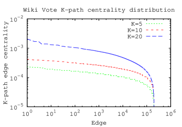
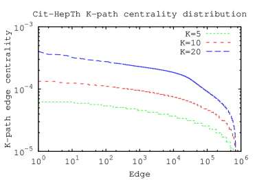
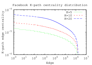
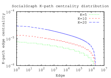
Figure 1: $\kappa$-paths centrality values distribution on different networks.

In the second experiment, we studied how the value of $\kappa$ impacted on edge centrality. In detail, we considered the datasets separately and applied the WERW-Kpath algorithm with $\kappa=5,10,20$. After that, for a fixed value of $\kappa$-path edge centrality $\overline{L}$, we computed the probability $P(\overline{L})$ of finding an edge with such a centrality value. The corresponding results are plotted in Figure 2 for the same datasets. As in the previous case, for each plot we adopted a log-log scale.

The analysis of this figure highlights some relevant facts. First of all, the heavy-tailed distribution in edge centrality emerges in presence of different values of $\kappa$. In other words, if we use different values of $\kappa$ the centrality indexes may change (see below); however, as emerges from Figure 1, for each considered dataset, the curves representing $\kappa$-path centrality values resemble straight and parallel lines with the exception of the latest part. This implies that, for a fixed value of $\kappa$, say $\kappa=5$, an edge $\overline{e}$ will have a particular centrality score. If $\kappa$ grows from 5 to 10 and, then, from 10 to 20, the centrality of $\overline{e}$ will be increased by a constant factor.

This leads us to hypothesize that a form of correlation should exist between the values of $L^{\kappa}(e)$ for different values of $\kappa$. To check whether this hypothesis were true, we performed a further experiment. In detail, we considered the above mentioned datasets and applied twice our algorithm on each of these datasets with two different values of $\kappa$, say $\kappa_{X}$ and $\kappa_{Y}$. Let us denote as $D_{X}$ (resp., $D_{Y}$) the distribution of edge centralities computed when $\kappa=\kappa_{X}$ (resp., $\kappa=\kappa_{Y}$). We compared $D_{X}$ and $D_{Y}$ and, to this purpose, we computed the Pearson Correlation coefficient $r_{\kappa_{X},\kappa_{Y}}$ of $D_{X}$ and $D_{Y}$. The Pearson Correlation Coefficient assumes that a linear relationship exists between $D_{X}$ and $D_{Y}$; such an assumption may be false because, in our scenario, we do not know if a linear relationship between $D_{X}$ and $D_{Y}$ exists and this could make the process of comparing $D_{X}$ and $D_{Y}$ unreliable. For instance, if $D_{X}$ and $D_{Y}$ were strongly correlated but both $D_{X}$ and $D_{Y}$ would contain some outliers, this would lead to significantly low values of $r_{\kappa_{X},\kappa_{Y}}$ and, in such a case, we should erroneously conclude that $D_{X}$ and $D_{Y}$ are weakly correlated. Due to these reasons, to make our analysis more robust, we computed two further metrics: the Spearman’s rank correlation coefficient $\rho_{\kappa_{X},\kappa_{Y}}$ and Kendall’s tau rank correlation coefficient $\tau_{\kappa_{X},\kappa_{Y}}$. Both these parameters are useful to determine whether two variables (in our case $D_{X}$ and $D_{Y}$) are related by a monotonic function, i.e., they are useful to identify to what extent when the former variable tend to increase the latter tends to increase too or to decrease.

The Spearman’s rank correlation coefficient is computed by converting the edge centralities into rank values (in such a way as to the edge with the highest centrality is ranked as first); subsequently, the Pearson Correlation Coefficient is computed on the rank values. The Spearman’s rank correlation coefficient ranges in $[-1,1]$.

The definition of the Kendall’s tau rank correlation coefficient is slightly complex; to this purpose, let us consider a pair of edges $e_{i}$ and $e_{j}$ and let us denote as $L^{\kappa_{X}}(e_{i})$ (resp., $L^{\kappa_{X}}(e_{j})$) and $L^{\kappa_{Y}}(e_{i})$ (resp., $L^{\kappa_{Y}}(e_{j})$) their centralities computed when $\kappa=\kappa_{X}$ and $\kappa=\kappa_{Y}$. The pairs $\langle L^{\kappa_{X}}(e_{i}),L^{\kappa_{X}}(e_{j})\rangle$ and $\langle L^{\kappa_{Y}}(e_{i}),L^{\kappa_{Y}}(e_{j})\rangle$ are said concordant if both $L^{\kappa_{X}}(e_{i})>L^{\kappa_{Y}}(e_{i})$ and $L^{\kappa_{X}}(e_{j})>L^{\kappa_{Y}}(e_{j})$ or $L^{\kappa_{X}}(e_{i})<L^{\kappa_{Y}}(e_{i})$ and $L^{\kappa_{X}}(e_{j})<L^{\kappa_{Y}}(e_{j})$. The same pairs are said discordant if both $L^{\kappa_{X}}(e_{i})>L^{\kappa_{Y}}(e_{i})$ and $L^{\kappa_{X}}(e_{j})<L^{\kappa_{Y}}(e_{j})$ or $L^{\kappa_{X}}(e_{i})<L^{\kappa_{Y}}(e_{i})$ and $L^{\kappa_{X}}(e_{j})>L^{\kappa_{Y}}(e_{j})$. The Kendall’s tau coefficient is equal to the ratio of the difference between the number of concordant and discordant pairs to the total number of pairs in distributions $D_{X}$ and $D_{Y}$ and it ranges in the real interval $[-1,1]$.

In Table 2 we report the outcomes of our experiment. Due to space limitations, we report four out of the nine datasets reported in Table 1 – the same of the previous experiment, namely “Wiki-vote”, “Cit-HepTh”, “Facebook” and “SocialGraph”. From Table 2, it emerges a strong agreement among the values returned by $r_{\kappa_{X},\kappa_{Y}}$, $\rho_{\kappa_{X},\kappa_{Y}}$ and $\tau_{\kappa_{X},\kappa_{Y}}$. In detail, all the metrics introduced above clearly indicate that there is a strong and positive correlation between $D_{X}$ and $D_{Y}$ for all datasets and for any pair of values $\kappa_{X}$ and $\kappa_{Y}$. Such a result highlights a nice property of our algorithm: the agreement between the two rankings produced for different values $\kappa_{X}$ and $\kappa_{Y}$ is the same; as a consequence, the edge having the highest centrality value when $\kappa=\kappa_{X}$ will be also the edge with the highest centrality value when $\kappa=\kappa_{Y}$. Therefore, our algorithm is robust against variations in the value of $\kappa$ and we can safely conclude that different values of $\kappa$ do not alter the distribution of edge centralities.

As previously observed, if $\kappa$ increases, the centrality index of an edge increases too (or, at least, it does not decrease). This has an intuitive explanation: if $\kappa$ increases, the WERW-KPath algorithm manages longer paths and, therefore, the chance that an edge is selected multiple times increases too. Each time an edge is selected, WERW-Kpath increases its weight by 1 and this increases the edge centrality values. Figure 1 show that if we augment $\kappa$, the distance between the highest and the lowest centrality value increase too. Therefore, in presence of low values of $\kappa$, edge centrality indexes tend to edge flatten in a small interval and it is harder to distinguish high centrality edges from low centrality ones. Vice versa, in presence of high values of $\kappa$, we are able to better discriminate edges with high centrality from edges with low centrality.

As a consequence, on one hand, it would be fine to fix $\kappa$ as high as possible. On the other hand, since the complexity of our algorithm is $O(\kappa|E|)$, large values of $\kappa$ negatively impact on the performance of our algorithm.

A good trade-off (suggested by the experiments showed in this section) is to fix $\kappa=20$.

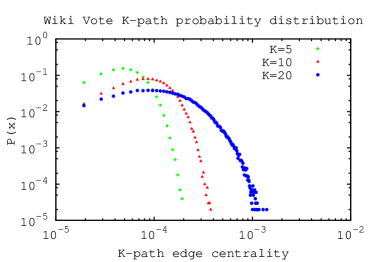
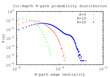
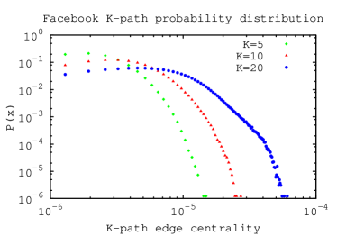
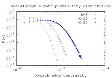
Figure 2: Effect of different $\kappa=5,10,20$ on networks described in Table 1.

Network	$\kappa_{X}$	$\kappa_{Y}$	$r_{\kappa_{X},\kappa_{Y}}$	$\rho_{\kappa_{X},\kappa_{Y}}$	$\tau_{\kappa_{X},\kappa_{Y}}$
Wiki-vote	5	10	0.9916	0.9897	0.9569
	10	20	0.9765	0.9976	0.9792
	20	5	0.9701	0.9925	0.9531
Cit-HepTh	5	10	0.9896	0.9907	0.9611
	10	20	0.9861	0.9971	0.9781
	20	5	0.9664	0.9924	0.9924
Facebook	5	10	0.9874	0.9810	0.9436
	10	20	0.9931	0.9952	0.9714
	20	5	0.9848	0.9858	0.9379
SocialGraph	5	10	0.9803	0.9772	0.9366
	10	20	0.9924	0.9910	0.9608
	20	5	0.9834	0.9811	0.9288

Table 2: Pearson ($r_{\kappa_{X},\kappa_{Y}}$), Spearman ($\rho_{\kappa_{X},\kappa_{Y}}$) and Kendall tau ($\tau_{\kappa_{X},\kappa_{Y}}$) rank correlation coefficients for pairs of distributions in Figure 2 (the p-value for all values is less than $10^{-10}$).

6.2 Assessing the Modularity

In this section we analyze the modularity of the partitions achieved by Louvain method, COPRA and OSLOM with and without the support of the WERW-Kpath algorithm.

The experiment has been carried out as follows: in a first stage we considered the original datasets (which can be regarded as unweighted graphs) and applied the Louvain method, COPRA and OSLOM on them. We computed the modularity achieved by each algorithm on each of these datasets. To make the notation simple we shall use the labels LM UW, CP UW and OS UW to denote, respectively, the Louvain method, COPRA and OSLOM applied on the unweighted, original, datasets.

In the second stage we pre-processed each of the 9 datasets reported in Table 1 by applying the WERW-Kpath algorithm with $\kappa=20$. Therefore, each graph was transformed into a weighted graph in which the weight of an edge was equal to its edge centrality. We applied again the three algorithms on the aforementioned datasets after adopting our strategy and we computed the achieved modularity. Similarly to previous case, we shall use the label LM W, CP W and OS W to denote, respectively, the Louvain method, COPRA and OSLOM applied on weighted, pre-processed, datasets.

The corresponding results are reported in Table 3. From the analysis of this table we conclude that:

1. As for LM, the usage of the WERW-Kpath algorithm always yields better results than using the original LM alone. In particular, the improvement of modularity is up 17.3%. It is interesting to observe that in the large-scale dataset (i.e., “SocialGraph”) a very high value of modularity was achieved by applying LM alone ($Q=0.891$). Neverthless, the WERW-KPath algorithm gives room for a further improvement ($Q=0.912$). This result is interesting because WERW-Kpath can yield relevant improvements also on large datasets for which the optimization of modularity becomes increasingly hard.

2. As for COPRA, there are two datasets (namely “CA-HepTh” and “CA-CondMat”) in which the performance of the community detection algorithm in conjunction with the WERW-Kpath algorithm produce a worse modularity than that achieved by COPRA alone. In all other cases, we report an increase of $Q$ ranging from 1.37% (“Facebook” dataset) to 9.02% (“Cit-HepTh” dataset). The combination of COPRA with the WERW-Kpath algorithm seems favorable for networks of medium size but it deteriorates for small and large networks. For instance, the increase of $Q$ is around 1.73% for the dataset called “Wiki-Vote” (7,115 vertices and 103,689 edges) and, as previously pointed out, 1.37% for the “Facebook” dataset (63,731 vertices and 1,545,684 edges). Such an improvement is better for “SocialGraph” because we pass from $Q=0.197$ achieved by COPRA alone to $Q=0.203$ with a gain of 3.04%. In such a case, however, the modularity achieved by COPRA is quite low in comparison with that of Louvain method and OSLOM and, therefore, such an improvement is not particularly relevant.

3. As for OSLOM, the improvements associated with the adoption of our method is less evident. In fact, we can observe that for 6 datasets out of 9 the joint usage of the WERW-KPath algorithm with OSLOM produce better results than those we would achieve if we would apply OSLOM alone. The improvement of $Q$ ranges from 2.8% to 7% (excluding the exceptional +17.4% for the dataset “Wiki-Vote”). To explain these results we can observe that OSLOM does not target at maximizing the network modularity but it relies on the idea that vertices can be ranked according to their likelihood of belonging to a community. Therefore, it is not surprising that the network modularity achieved by OSLOM is significantly less than that achieved by the Louvain method. However, it is worth observing that the gain in modularity deriving from the usage of the WERW-Kpath algorithm is almost uniform: for instance, the increase of $Q$ due to the coupling of WERW-Kpath with OSLOM is 7% for the dataset called “CA-AstroPh”, 6.21% for the dataset called “CA-CondMat”, 6.66% for the dataset called “Cit-HepTh” and 4.82% for the dataset called “SocialGraph”. This implies that the joint usage of WERW-KPath is not influenced (or at least is weakly influenced) by the size of the input dataset.

Network	LM UW	LM W	CP UW	CP W	OS UW	OS W
Wiki-Vote	0.423	0.445 [+5.2%]	0.693	0.705 [+1.7%]	0.316	0.371 [+17.4%]
CA-HepTh	0.772	0.806 [+4.4%]	0.768	0.649 [-18.4%]	0.653	0.632 [-3.3%]
CA-HepPh	0.656	0.760 [+15.8%]	0.754	0.777 [+3.1%]	0.675	0.669 [-0.01%]
CA-AstroPh	0.627	0.663 [+5.7%]	0.577	0.614 [+6.4%]	0.596	0.638 [+7.0%]
CA-CondMat	0.731	0.768 [+5.1%]	0.616	0.515 [-19.6%]	0.692	0.735 [+6.2%]
Cit-HepTh	0.642	0.644 [+0.1%]	0.665	0.725 [+9.0%]	0.433	0.462 [+6.7%]
Email-Enron	0.602	0.706 [+17.3%]	0.768	0.799 [+4.0%]	0.449	0.432 [-4.0%]
Facebook	0.626	0.664 [+6.1%]	0.799	0.810 [+1.4%]	0.391	0.402 [+2.8%]
SocialGraph	0.891	0.912 [+2.4%]	0.197	0.203 [+3.0%]	0.456	0.478 [+4.8%]

Table 3: Network Modularity of Louvain method, COPRA and OSLOM with and without our approach ($\kappa=20$). Improved values are highlighted in bold, reduced values are emphasized and the improvement/loss is reported in brackets.

The results reported in this section indicates that some community detection methods (like LM) significantly benefit from our edge weighting strategies; for COPRA and OSLOM our method brings some advantage but the improvement in modularity is less evident than in LM. Such a behavior can be explained in terms of the properties and behavior of the LM, COPRA and OSLOM algorithms.

As emerges from Section 5.1, LM tries to optimize in a greedy fashion the modularity function $Q$ defined in Equation 1. The $Q$ function is the sum of terms of the form $\Delta_{ij}=\left(A_{ij}-\frac{k_{i}\cdot k_{j}}{2m}\right)\delta(C_{i},C_{j})$. Let us consider a pair of vertices $i$ and $j$ and assume that an edge linking them exists. By exploiting LM in conjunction with our WERW-Kpath algorithm, $A_{ij}$ is a real number in [0,1]; if the WERW-Kpath algorithm is not applied, $A_{ij}\in{0,1}$ and it equals 1 if and only if there is an edge linking $i$ and $j$. In such a case the term $\Delta_{ij}$ reads $\hat{\Delta_{ij}}=\left(1-\frac{k_{i}\cdot k_{j}}{2m}\right)\delta(C_{i},C_{j})$. Therefore, the less $k_{i}$ (resp., $k_{j}$) the higher $\hat{\Delta_{ij}}$: this implies that LM tends to put in the same community vertices at low degree even if such a choice could be not optimal at the global level. By contrast, the usage of non-binary weights on edges provides a higher level of flexibility to the algorithm and this ultimately explains the improvements in the values of $Q$.

As for COPRA and OSLOM, the discussion proposed in Sections 5.2 and 5.3 explains that these algorithms deeply differ each other. Despite these deep differences, they share a relevant similarity: in both of them, a vertex $v$ is assigned to a community depending on the fact that a large part of the neighboring vertices of $v$ belong or not to that community. So, for instance, in COPRA we compute the belonging coefficient of $v$ to a community $C$ depending on the belonging coefficient to $C$ of its neighboring vertices. In OSLOM, we compute the number of links joining $v$ with vertices located inside $C$ and if such a number is higher than that we would expect, we decide to put $v$ in $C$. In both COPRA and OSLOM, the criterium to decide if a vertex has to be included in a community depends on the number of its neighboring vertices belonging to that community and, ultimately, on the number of edges linking $v$ with vertices located in $C$. Therefore, weights on edges have a small (or negligible) influence in deciding to assign a vertex to a community.

6.3 Quality Assessment

In this section we analyze the quality of the communities detected by our approach in conjunction with LM, COPRA and OSLOM.

To assess the quality of the results, we adopted a measure called Normalized Mutual Information - NMI proposed by Danon et al. in 2005 [9] which is rooted in Information Theory. Such a measure assumes that, given a graph $G$, a ground truth is available to verify what are the communities (said real communities) in $G$ and what are their features. Let us denote as $A$ the true community structure of $G$ and suppose that $G$ consist of $c_{A}$ communities. Let us consider a community detection algorithm $\cal A$. Let us run $\cal A$ on $G$ and assume that it identifies a community structure $B$ consisting of $c_{B}$ communities. We define a $c_{A}\times c_{B}$ matrix – said confusion matrix – $CM$ such that each row of $CM$ corresponds to a community in $A$ whereas each column of $CM$ is associated with a community in $B$. The generic element $CM_{ij}$ is equal to the number of elements of the real $i$-th community which are also present in the $j$-th community found by the algorithm. Starting by this definition, the normalized mutual information is defined as

$$NMI(A,B)=\frac{-2\sum_{i=1}^{c_{A}}\sum_{j=1}^{c_{B}}N_{ij}\log\left(\frac{N_{ij}N}{N_{i\cdot}N_{\cdot j}}\right)}{\sum_{i=1}^{c_{A}}N_{i\cdot}\log\left(\frac{N_{i\cdot}}{N}\right)+\sum_{j=1}^{c_{B}}N_{\cdot j}\log\left(\frac{N_{\cdot j}}{N}\right)}$$ (11)

being $N_{i\cdot}$ (resp., $N_{\cdot j}$) the sum of the elements in the $i$-th row (resp., $j$-th column) of the confusion matrix. If the algorithm $\cal A$ would work perfectly, then for each found community $j$, it would exist a real community $i$ exactly coinciding with $j$. In such a case, it is possible to show that $NMI(A,B)$ is exactly equal to 1 [9]. By contrast, if the communities detected by $\cal A$ are totally independent of the real communities (e.g. if we assume to put all the nodes of the network into a single community) then it is possible to show that the NMI is equal to 0. The NMI, therefore, ranges from 0 to 1 and the higher the value, the better the algorithm works.

The computation of NMI is however challenging for real-life networks because no ground truth is usually available to assess what are the communities in $G$ and what are their features. Therefore, to perform our tests, we need to consider a set of artificially generated networks whose structural properties are compliant with those existing in real networks.

A tool for generating artificial networks resembling real ones has been proposed in [35] and it has been exploited in our tests. The user is required to provide the following parameters to generate artificial networks: (i) Number of Vertices and Average Vertex Degree. The user is allowed to specify the number $N$ of vertices in the network as well as the average degree $\langle k\rangle$ of each vertex. (ii) Power Law exponent in vertex degree distribution. The user specifies a parameter $\gamma$ such that the vertex degree distribution follows a power law such as $P(k)\propto k^{-\gamma}$. In addition, the average degree of a vertex is fixed to be equal to $\langle k\rangle$. (iii) Power Law exponent in community size distribution. The user specifies a parameter $\beta$ and communities are generated so that the size of each community (i.e., the number of vertices composing it) follows a power law defined as $f(x)\propto x^{-\beta}$. The sum of the sizes of all the communities is constrained to be equal to $N$. In addition, the procedure for generating communities ensures that any node is included in at least a community, independently of its degree. (iv) Mixing parameter. The user specifies a parameter $\mu\in(0,1)$ such that each vertex shares a fraction $1-\mu$ of its edges with vertices outside its community and $\mu$ edges with vertices residing in its community. The parameter $\mu$ is called mixing parameter. Note that the mixing parameter assignment $\mu=0.5$ represents the tipping point beyond which the communities are no longer defined in the strong sense, that is that each vertex has more neighbors in the community to which it is assigned, rather than outside.

In our tests we adopted the same configuration reported in [35], i.e.,: (i) $N=1000$ vertices; (ii) four pair of values for $\gamma$ and $\beta$ were considered, namely: $(\gamma,\beta)$ = (2,1), (2,2), (3,1), (3,2); (iii) three values of average degree were considered, namely $\langle k\rangle=15,20,25$; (iv) six values of $\mu$ were considered, namely $\mu=0.1,\dots,0.6$. This allowed us to generate an overall number of $4\cdot 3\cdot 6=72$ artificial test networks.

We computed the NMI achieved by applying LM, COPRA and OSLOM, on the unweighted networks as they were generated by the benchmark, averaging obtained results over 10 runs of each algorithm. Therefore, we applied the same algorithms to the weighted networks after the adoption of our network weighting strategy, once again averaging results over 10 runs. As suggested in Section 6.2, we fixed $\kappa=20$ to compute edge centralities.

The achieved results are reported in Table 4 for $\langle k\rangle=20$. We also considered other values for average degree, namely $\langle k\rangle=15$ and $\langle k\rangle=25$ and the results we obtained were quite similar each other and inline with those obtained when $\langle k\rangle=20$; therefore, due to space limitation, we report in Table 4 only the NMI values obtained when $\langle k\rangle=20$.

Method	$\mu=0.1$	$0.2$	$0.3$	$0.4$	$0.5$	$0.6$
$\gamma=2,\beta=1$
LM UW	0.917	0.853	0.769	0.732	0.591	0.486
LM W	0.931	0.882	0.817	0.789	0.599	0.444
CP UW	0.868	0.901	0.841	0.868	0.691	0.021
CP W	0.879	0.900	0.905	0.856	0.846	0.021
OS UW	0.699	0.703	0.705	0.694	0.658	0.438
OS W	0.700	0.704	0.707	0.695	0.668	0.501
$\gamma=2,\beta=2$
LM UW	0.815	0.633	0.664	0.428	0.503	0.334
LM W	0.886	0.704	0.632	0.519	0.444	0.377
CP UW	0.849	0.893	0.838	0.809	0.726	0.028
CP W	0.904	0.852	0.886	0.759	0.738	0.028
OS UW	0.669	0.637	0.629	0.633	0.583	0.462
OS W	0.669	0.637	0.637	0.629	0.602	0.505
$\gamma=3,\beta=1$
LM UW	0.973	0.867	0.800	0.773	0.677	0.527
LM W	0.978	0.872	0.806	0.739	0.712	0.404
CP UW	0.917	0.888	0.876	0.875	0.727	0.018
CP W	0.927	0.892	0.892	0.913	0.786	0.018
OS UW	0.741	0.711	0.700	0.712	0.708	0.299
OS W	0.741	0.712	0.700	0.712	0.711	0.415
$\gamma=3,\beta=2$
LM UW	0.936	0.788	0.692	0.563	0.532	0.411
LM W	0.947	0.745	0.749	0.633	0.584	0.405
CP UW	0.881	0.892	0.900	0.885	0.844	0.023
CP W	0.911	0.875	0.899	0.889	0.770	0.023
OS UW	0.697	0.672	0.665	0.671	0.652	0.397
OS W	0.697	0.672	0.665	0.672	0.652	0.538

Table 4: Louvain method (LM), COPRA (CP) and OSLOM (OS) NMI performance for artificial networks with average degree $\langle k\rangle=20$. Statistically significant improvements (p-value $<0.001$) are highlighted in bold.

From the analysis of this table, we can draw the following conclusions:

1. If $\mu$ is low (i.e., $\mu=0.1$ or $\mu=0.2$), all the three approaches achieve a high NMI both with and without our weighting strategy. By contrast, for large values of $\mu$ (for example $\mu=0.6$), the NMI deteriorates (especially for COPRA). In particular, if $\mu>0.5$ a vertex has more neighbors outside the community to which it is assigned than in the community itself. Among the three methods, COPRA suffers the increase of $\mu$ more than Louvain method and OSLOM. In fact, if $\mu$ is around 0.1-0.2, the NMI achieved by COPRA is in line with that of Louvain method and in general it is quite high (between 0.849 and 0.917) but if $\mu$ tends to 0.6 its NMI decreases of about 90% (and its values are around 0.018-0.023). This depends on the features of COPRA: in fact, a vertex $v$ is assigned to a community $C$ if most of its neighbors already belong to $C$. Of course, such an assignment is problematic for large values of $\mu$ because, as already observed, the neighbors of $v$ could be equally split across multiple communities.

2. It is worth observing that coupling Louvain method, COPRA and OSLOM with our strategy generally provides also an increase of NMI. To assess if the improvement provided by our method is significant or not, we carried out a t-test. We considered a p-value lesser than 0.001 to determine, over 10 runs of each algorithm ($df=9$), if the obtained increment was statistically significant or not. According to this test, significant increments are reported in bold in Table 4. It emerges that the increase of NMI is generally extremely significant pairing the Louvain method with our weighting strategy (in particular, for $\gamma=2$ this choice is able to guarantee significant improvements with low values of $\mu$, while for $\gamma=3$ the increment is obtained also for high values of $\mu$.) Regarding the choice of COPRA paired with our strategy, we also obtain statistically significant improvements of NMI with all assignements of $\gamma$ and $\beta$, in particular with medium/high values of $\mu$. Differently, by considering OSLOM, the only extremely significant improvement in NMI is obtained while considering $\mu=0.6$, but this increase is neat and appears in all possible configurations of $\gamma$ and $\beta$.

3. For a fixed value of $\gamma$ and $\mu$, we observe that the NMI achieved by the Louvain method decreases if $\beta$ ranges from 1 to 2. If $\beta$ gets larger, there are few communities containing a large number of vertices and a large number of communities which have roughly the same size because they contain few vertices. These communities are hard to find due to the so-called resolution limit [19]: in particular, it is possible to show that community detection algorithms based on the principle of modularity maximization may fail to find communities containing less than $\sqrt{|E|/2}$ edges, being $|E|$ the number of edges in the entire network.

   However, a big result emerges from Table 4: if we couple LM with the WERW-Kpath algorithm then the decay in NMI is softened. This depends on the different definition of the modularity function that the Louvain method attempts to optimize: in the case of weighted network, in fact, the term $A_{ij}$ is no longer 0 or 1 depending if an edge links the vertices $i$ and $j$ but it is a real number in [0,1] defining the strength of their links. The definition of the $Q$ function, therefore, is more precise and this allows higher values of $Q$ to be achieved.

7 Related Works

In this section we describe some works related to our research.

First of all, we point out that an early version of the WERW-Kpath algorithm discussed appeared in [10]. We brought in some little modifications to the original WERW-KPath algorithm to achieve more solid results from a theoretical standpoint on the behavior of the algorithms itself. In detail, in the algorithm presented in [10] the weight $\omega(e)$ of $e$ is proportional to the number of times $e$ is selected by the algorithm. This weight is interpreted as the edge centrality of $e$, i.e., we set $\hat{L}_{k}(e)=\omega(e)$: therefore, $\hat{L}_{k}(e)$ represents the frequency of selecting $e$ by means of random simple paths consisting of at most $\kappa$ edges. By contrast, in this paper, the weight $\omega(e)$ of $e$ counts how many times $e$ is selected and the edge centrality $\hat{L}_{k}(e)$ returned by the algorithm is equal to $\omega(e)$ divided by the number of trials $\rho$ performed by the algorithm. In this case, $\hat{L}_{k}(e)$ represents the probability of selecting $e$. This has relevant practical consequences. In fact, in [10], we were able to prove that the edge $\omega(e)$ lies in a closed interval of the form $[\xi_{1}L_{\kappa}(e),\xi_{2}L_{\kappa}(e)]$, being $\xi_{1}$ and $\xi_{2}$ two real constants. However, we were not able to provide an estimation of $\xi_{1}$ and $\xi_{2}$, and, then, to quantify the approximation error associated with the estimation of $L_{\kappa}(e)$. In addition, we were not able to relate the number $\rho$ of trials carried out by the algorithm to the accuracy of the algorithm in approximating the actual edge centrality values. Some design considerations (later supported by experimental trials) suggested us to set $\rho=|E|-1$. Both these limitations have been addressed in the current version of the algorithm by means of Theorem 4.2 and Corollary 4.3. In fact, by means of Theorem 4.2, we provide tight bounds on the probability that $|\hat{L}_{\kappa}(e)-L_{\kappa}(e)|$ exceeds a given threshold and, by means of Corollary 4.3 and the subsequent reasoning we showed that, in case of real networks, a number of iterations equal to the number of vertices in the network was enough to provide accurate results.

However, the main novelty introduced in this paper is that we showed how to apply the WERW-Kpath algorithm to a non-trivial problem, i.e., the task of finding communities in networks. To the best of our knowledge, there are few works proposing to weight edges in a network to improve the quality of the community detection process.

One of the first approach to weighting edges was proposed in [33]. In that paper, the authors propose a modified version of the Girvan-Newman algorithm called Newman Fast. In particular, given an unweighted, undirected graph $G$, each edge $e_{ij}$ connecting a pair of vertices $i$ and $j$ is weighted. The weight of $e_{ij}$ is the normalized product of two terms: the former is the inverse of the edge betweenness associated with $e_{ij}$ whereas the latter (called common neighbor ratio) is the normalized number of vertices which are linked to both $i$ and $j$. After that weighting step has been carried out, the Newman Fast algorithm attempts to minimize the function $\tilde{Q}$ defined as

$$\tilde{Q}=\sum_{l}(e_{ll}-a_{l}^{2})$$

The authors define $e_{lp}$ equal to half of the sum of the weights of the edges that start from vertices in community $l$ and end in vertices located in community $p$ over the sum of the weights of all the edges in the network. Therefore, $e_{ll}$ is the sum of the weights of the edges contained within the community $l$. The parameter $a_{l}$ is defined as $a_{l}=\sum_{k}e_{lk}$. The algorithm proceeds adopting a greedy strategy to maximize $\tilde{Q}$: initially, each vertex forms a community and communities are merged so that to increase the value of $\tilde{Q}$. The process stops when no further improvement of $\tilde{Q}$ can be achieved or all the vertices have been inserted into a single community.

An improvement of the approach of [33] was presented, by the same authors, in [34]. In that paper the authors suggested a slightly different weighting schema in which the contributions of edge betweenness and common neighbor ratio are combined through two weights $\alpha$ and $\beta$. The authors suggest to tune $\alpha$ and $\beta$ so that to maximize the variance in edge distribution.

There are some differences between our approach and that of [33]. In detail, in the approach of [33], the edge weight is the product of two terms: the former is the edge betweenness, which is a global parameter (i.e., its computation requires to know the whole network topology) and the common neighbor ratio, which is a local parameter (i.e., it can be computed by knowing only the neighbors of two vertices). Our $\kappa$-path centrality, instead, lies between local and global measures because it can be computed by considering random paths of length at most $\kappa$. Therefore, if $\kappa$ is kept low (resp., high) the edge centrality configure itself as a local (resp., global) measure. As a further difference, the edge weighting procedure outlined in [33, 34] has been used to design a modified version of $Q$ and a greedy algorithm to optimize it. By contrast, in our approach we do not focus on any specific community detection algorithm and, therefore, our approach can be used also with algorithms like COPRA or OSLOM which do not attempt at maximizing modularity. In general, our strategy can be paired up with any community detection algorithm handling weighted networks.

A further, interesting study, is presented in [2]. In that paper the authors studied the aforementioned problem of resolution limit [19]. In [19], the authors showed that the size of the smallest community which can be detected is $\sqrt{|E|/2}$, being $|E|$ the number of edges in the network. In [2] the authors pointed out that by weighting a network the resolution limit amounts to $\sqrt{W\varepsilon/2}$, being $W$ the sum of the weights in the network and $\varepsilon$ the maximum weight of an edge connecting vertices located in two different communities. Therefore, a wise choice of weights can significantly lower the resolution limit. The authors suggested a weighting schema in which the weight of an edge depends on the number of cycles of length $k$ containing that edge, being $k$ a fixed integer. The authors provides a modified version of the Clauset, Newman and Moore algorithm [6] capable of taking into account edge weights.

Our approach differs from that proposed in [2]. In fact, we leverage on random walks to compute edge weight whereas the approach of [2] relies on the identification of cycles of length $k$. Unfortunately, the identification of these cycles can be very time expensive as soon as $k$ gets large. On the contrary, we proved both theoretically and experimentally that our strategy scales very well also if applied to large networks.

8 Conclusions

In this paper we discussed an algorithm, called WERW-Kpath, to compute edge centralities in networks and we showed that the strategy of weighting edges can generate a significant improvement in the process of discovering communities. The WERW-Kpath algorithm exploits random walks of bounded length to compute edge centralities. We provided a theoretical analysis of the behavior of the WERW-Kpath algorithm and we showed how to use it in conjunction with already existing community detection algorithm. We studied the merits and weaknesses of the WERW-Kpath algorithm by coupling it with three state-of-the-art algorithms, namely Louvain Method, COPRA and OSLOM. Experiments carried out on real networks show that our approach is able to improve the modularity of the community structure detected by the algorithms mentioned above and the improvement up to 17.3%. We carried out also experiments on artificial networks: experiments showed that coupling Louvain method, COPRA and OSLOM with our strategy generally provides an increase of the Normalized Mutual Information.

As for future work, we plan to implement a multi-threaded version of the WERW-Kpath algorithm so that we can simulate multiple random walks on the network in parallel. We plan to experimentally study the computational improvements deriving from this choice. A further research direction includes the creation of a friendship recommender system which suggests new possible connections to the users of a very large-scale online social network, based on the communities they belong to.

References

- [1] T. Alahakoon, R. Tripathi, N. Kourtellis, R. Simha, and A. Iamnitchi. K-path centrality: A new centrality measure in social networks. In Proc. of 4th Workshop on Social Network Systems, pages 1–6, 2011.
- [2] J. Berry, B. Hendrickson, R. LaViolette, and C. Phillips. Tolerating the community detection resolution limit with edge weighting. Physical Review E, 83(5):056119, 2011.
- [3] V. Blondel, J. Guillaume, R. Lambiotte, and E. Lefebvre. Fast unfolding of communities in large networks. Journal of Statistical Mechanics: Theory and Experiment, page P10008, 2008.
- [4] U. Brandes. A faster algorithm for betweenness centrality. Journal of Mathematical Sociology, 25(2):163–177, 2001.
- [5] U. Brandes, D. Delling, M. Gaertler, R. Görke, M. Hoefer, Z. Nikoloski, and D. Wagner. On finding graph clusterings with maximum modularity. In Graph-Theoretic Concepts in Computer Science, pages 121–132, 2007.
- [6] A. Clauset, M. Newman, and C. Moore. Finding community structure in very large networks. Physical Review E, 70(6):66111, 2004.
- [7] V. Chua, J. Madej, and B. Wellmann. Personal Communities: The World According To Me. The SAGE Handbook of Social Network Analysis, Sage Publications Ltd, California, 2005.
- [8] T. Cormen, C. Leiserson, R. Rivest, and C. Stein. Introduction to Algorithms. The MIT Press, 2001.
- [9] L. Danon, A. Diaz-Guilera, J. Duch, and A. Arenas. Comparing community structure identification. Journal of Statistical Mechanics: Theory and Experiment, page P09008, 2005.
- [10] P. De Meo, E. Ferrara, G. Fiumara, and A. Ricciardello. A Novel Measure of Edge Centrality in Social Networks. Knowledge-based Systems, 30:136–150, 2012.
- [11] P. De Meo, E. Ferrara, G. Fiumara, A. Provetti. Generalized louvain method for community detection in large networks. In Proc. 11th International Conference on Intelligent Systems Design and Applications, pages 88–93, 2011.
- [12] P. De Meo, A. Nocera, G. Terracina, and D. Ursino. Recommendation of similar users, resources and social networks in a social internetworking scenario. Information Sciences, 181(7):1285–1305, 2011.
- [13] J. Duch and A. Arenas. Community detection in complex networks using extremal optimization. Physical Review E, 72(2):27104, 2005.
- [14] R. I. M. Dunbar. Neocortex size as a constraint on group size in primates. Journal of Human Evolution, 22(6):469–493, 1992.
- [15] C. Durugbo, W. Hutabarat, A. Tiwari, and J. Alcock. Modelling collaboration using complex networks. Information Sciences, 181(15):3143–3161, 2011.
- [16] E. Ferrara. A large-scale community structure analysis in Facebook. Arxiv preprint arXiv:1106.2503v4, 2012.
- [17] E. Ferrara. Community Structure Discovery in Facebook. International Journal of Social Network Mining, 1:67–90, 2012.
- [18] S. Fortunato. Community detection in graphs. Physics Reports, 486(3-5):75–174, 2010.
- [19] S. Fortunato and M. Barthélemy. Resolution limit in community detection. Proceedings of the National Academy of Sciences, 104(1):36, 2007.
- [20] S. Fortunato, V. Latora, and M. Marchiori. Method to find community structures based on information centrality. Physical Review E, 70(5):056104, 2004.
- [21] Grabowicz P, Ramasco J, Moro E, Pujol J, Eguiluz V. Social features of online networks: The strength of intermediary ties in online social media. PloS one 2012, 7:e29358.
- [22] N. Friedkin. Horizons of observability and limits of informal control in organizations. Social Forces, 62(1):55–77, 1983.
- [23] M. Girvan and M. Newman. Community structure in social and biological networks. Proceedings of the National Academy of Sciences, 99(12):7821, 2002.
- [24] M. Gjoka, M. Kurant, C. Butts, and A. Markopoulou. Walking in Facebook: A case study of unbiased sampling of osns. In INFOCOM, 2010 Proceedings IEEE, pages 1–9. Ieee, 2010.
- [25] S. Gregory. An algorithm to find overlapping community structure in networks. Knowledge Discovery in Databases: PKDD 2007, pages 91–102, 2007.
- [26] S. Grunwald, A. Speer, J. Ackermann, and I. Koch. Petri net modelling of gene regulation of the duchenne muscular dystrophy. Biosystems, 92(2):189–205, 2008.
- [27] R. Guimera and L. N. Amaral. Functional cartography of complex metabolic networks. Nature, 433(7028):895–900, 2005.
- [28] R. Guimera, M. Sales-Pardo, and L. Amaral. Modularity from fluctuations in random graphs and complex networks. Physical Review E, 70(2):025101, 2004.
- [29] L. Hagen and A. Kahng. New spectral methods for ratio cut partitioning and clustering. Computer-Aided Design of Integrated Circuits and Systems, IEEE Transactions on, 11(9):1074–1085, 2002.
- [30] J. Han and M. Kamber. Data Mining: Concepts and Techniques - Second Edition. Morgan Kaufmann Publishers, 2006.
- [31] W. Hoeffding. Probability inequalities for sums of bounded random variables. Journal of the American Statistical Association, pages 13–30, 1963.
- [32] R. Johnston, and P. Charles. Social Networks, Geography and Neighbourhood Effects. The SAGE Handbook of Social Network Analysis, SAGE Publications, California, 2005.
- [33] A. Khadivi, A. Rad, and M. Hasler. Community detection enhancement in networks using proper weighting and partial synchronization. In Circuits and Systems (ISCAS), Proceedings of 2010 IEEE International Symposium on, pages 3777–3780. IEEE, 2010.
- [34] A. Khadivi, A. Rad, and M. Hasler. Network community-detection enhancement by proper weighting. Physical Review E, 83(4):046104, 2011.
- [35] A. Lancichinetti and F. Radicchi. Benchmark graphs for testing community detection algorithms. Physical Review E, 78(4):046110, 2008.
- [36] A. Lancichinetti, F. Radicchi, J. Ramasco, and S. Fortunato. Finding statistically significant communities in networks. PloS one, 6(4):e18961, 2011.
- [37] J. Leskovec and C. Faloutsos. Sampling from large graphs. In Proc. 12th ACM SIGKDD international conference on Knowledge discovery and data mining, pages 631–636, 2006.
- [38] Z. Li, S. Zhang, R. Wang, X. Zhang, and L. Chen. Quantitative function for community detection. Physical Review E, 77(3):036109, 2008.
- [39] N. Lin, and M. Dumin. Access to occupations through social ties. Social Networks, 8(4):365–385, 1986.
- [40] B. Mirkin and S. Nascimento. Additive spectral method for fuzzy cluster analysis of similarity data including community structure and affinity matrices. Information Sciences, 183(1):16–34, 2012.
- [41] M. Newman. A measure of betweenness centrality based on random walks. Social networks, 27(1):39–54, 2005.
- [42] M. Newman and M. Girvan. Finding and evaluating community structure in networks. Physical Review E, 69(2):26113, 2004.
- [43] A. Ng, M. Jordan, and Y. Weiss. On Spectral Clustering: Analysis and an algorithm. In Advances in Neural Information Processing Systems 14, 2001.
- [44] G. Palla, I. Derenyi, I. Farkas, and T. Vicsek. Uncovering the overlapping community structure of complex networks in nature and society. Nature, 435(7043):814–818, 2005.
- [45] M. Porter, J. Onnela, and P. Mucha. Communities in networks. Notices of the American Mathematical Society, 56(9):1082–1097, 2009.
- [46] U. Raghavan, R. Albert, and S. Kumara. Near linear time algorithm to detect community structures in large-scale networks. Physical Review E, 76(3):036106, 2007.
- [47] D. Shah and T. Zaman. Community detection in networks: The leader-follower algorithm. In Proc. Workshop on Networks Across Disciplines: Theory and Applications, pages 1–8, 2010.
- [48] B. Viswanath, A. Mislove, M. Cha, and K. P. Gummadi. On the evolution of user interaction in Facebook. In Proc. 2nd ACM SIGCOMM Workshop on Social Networks, 2009.
- [49] C. Von Mering, E. Zdobnov, S. Tsoka, F. Ciccarelli, J. Pereira-Leal, C. Ouzounis, and P. Bork. Genome evolution reveals biochemical networks and functional modules. Proceedings of the National Academy of Sciences, 100(26):15428, 2003.
- [50] Y. Wei and C. Cheng. Towards efficient hierarchical designs by ratio cut partitioning. In Proc. IEEE International Conference on Computer-Aided Design, pages 298–301, 1989.