The coupling between internal waves and shear-induced turbulence in stellar radiation zones: the critical layers

Abstract

Context. Internal gravity waves (hereafter IGW) are known as one of the candidates for explaining the angular velocity profile in the Sun and in solar-type main-sequence and evolved stars, due to their role in the transport of angular momentum. Our bringing concerns critical layers, a process poorly explored in stellar physics, defined as the location where the local relative frequency of a given wave to the rotational frequency of the fluid tends to zero (i. e. that corresponds to co-rotation resonances).

Aims. IGW propagate through stably-stratified radiative regions, where they extract or deposit angular momentum through two processes: radiative and viscous dampings and critical layers. Our goal is to obtain a complete picture of the effects of this latters.

Methods. First, we expose a mathematical resolution of the equation of propagation for IGWs in adiabatic and non-adiabatic cases near critical layers. Then, the use of a dynamical stellar evolution code, which treats the secular transport of angular momentum, allows us to apply these results to the case of a solar-like star.

Results. The analysis reveals two cases depending on the value of the Richardson number at critical layers: a stable one, where IGWs are attenuated as they pass through a critical level, and an unstable turbulent case where they can be reflected/transmitted by the critical level with a coefficient larger than one. Such over-reflection/transmission can have strong implications on our vision of angular momentum transport in stellar interiors.

Conclusions. This paper highlights the existence of two regimes defining the interaction between an IGW and a critical layer. An application exposes the effect of the first regime, showing a strengthening of the damping of the wave. Moreover, this work opens new ways concerning the coupling between IGWs and shear instabilities in stellar interiors.

1 Introduction

Thanks to helio- and asteroseismology, we are able to extract a huge amount of informations about solar and stellar structures and compositions (e.g. Turck-Chièze & Couvidat (2011); Aerts et al. (2010)) and their internal differential rotation profile (Garcia et al., 2007; Beck et al., 2012; Deheuvels et al., 2012). We know that internal rotation modifies the stellar structure since it generates flows, instabilities and chemical elements mixing, which modify stars evolution, for example their lifetime and their nucleosynthetic properties (e.g. Maeder, 2009, and references therein). Moreover, in order to understand the obtained solar/stellar rotation profiles and the related rotational history, it is essential to develop a complete theory incorporating the different angular momentum transport mechanisms occuring in stellar interiors (e.g. Mathis, 2010, and references therein). In this context, one legitimely asks the question about the origin of the internal rotation profiles. Four main processes are responsible, in different ways, for the secular angular momentum transport in radiative interiors. First, a large-scale meridional circulation is driven by structural adjustments of stars, external applied torques and internal stresses (e.g. Zahn, 1992; Mathis & Zahn, 2004; Decressin et al., 2009). Next, rotation profiles may be subject to different hydrodynamical shear and baroclinic instabilities and turbulence (e.g. Knobloch & Spruit, 1982; Talon & Zahn, 1997; Maeder, 2003; Mathis et al., 2004). Then, fossil magnetic fields, trapped during early-phases of stellar evolution once radiation zones have been formed (Braithwaite & Spruit, 2004; Duez & Mathis, 2010), can transport angular momentum through large-scale torques and Maxwell stresses (e.g. Gough & McIntyre, 1998; Mathis & Zahn, 2005; Garaud & Garaud, 2008; Strugarek et al., 2011). Finally, IGWs excited at the convection/radiation boundaries constitute the fourth mechanism able to transport angular momentum over large distances in stellar radiation zones (e.g. Press, 1981; Goldreich & Nicholson, 1989; Schatzman, 1993; Zahn et al., 1997; Talon & Charbonnel, 2005; Mathis & de Brye, 2012). Note that all these processes are not necessarily present at the same time everywhere in the H.-R. diagram. Moreover, they act on various characteristic timescales in stars of different masses and ages.

The object of this paper is the propagation of IGWs and the way they interact with the shear (i.e. the differential rotation) of the surrounding fluid. They are common in the terrestrial atmosphere and oceans (Eckart, 1961; Chapman & Lindzen, 1970), that is why they are pretty well known in Geophysics. We will use this advantage for their study in the stellar case. We here draw attention to the mechanism whereby IGWs exchange energy with the mean flow, independently from other dissipative processes such as thermal and viscous diffusion. Indeed, when the frequency of excited waves is of the same order as the angular velocity of the fluid (we will see the accurate definition later), a phenomenon of resonance occurs, which affects the properties of both the wave and the shear of the surrounding fluid. This phenomenon is called a critical layer. Under the assumption of a perfect fluid (neither heat conductor nor viscous), Booker & Bretherton (1967) and Lindzen & Barker (1985) have provided first results about critical layers in the geophysical case. They have shown that, depending on the value of the Richardson number of the fluid, which compares the relative strength of the shear and of the stable stratification (see Eq. 3), the waves might be either attenuated or reflected by the critical layer. This reflection may even be an over-reflection together with an over-transmission (see also Sutherland & Yewchuk (2004) for a laboratory evidence). In the same time, Koppel (1964); Hazel (1967); Baldwin & Roberts (1970); Van Duin & Kelder (1986) have completed this work in taking into account the conduction of heat and the viscosity of the fluid. Surprinsingly, their conclusions about the role of critical layers are identical. However, all these authors have produced their study in cartesian coordinates, assuming that the stiffness of the domain was thin enough to neglect its curvature. In the case of stellar radiation zones where critical layers may play an important role (e.g. Barker & Ogilvie, 2010; Barker, 2011; Rogers et al., 2012), these equations should thus be generalized to the case of spherical coordinates to be able to treat deep spherical shells.

Therefore, after exposing our notations and assumptions (§2.), we present a complete mathematical study of critical layers in the case of a perfect fluid (§3.) and of a non-perfect fluid (§4.) in spherical geometry. Then, we determine the related mean vertical flux of angular momentum transported by IGWs (§5.). Next, we implement our theoretical results in the dynamical stellar evolution code STAREVOL and we apply our formalism to the evolution of a one solar-mass star (§6.). Finally, we present the conclusion and perspectives of this work (§7.).

2 Definition, notations and hypotheses

The star we consider is composed (at least) with a convective and a radiative region. IGWs are excited at the boundary between these two regions. They propagate in the radiative zone and are evanescent in the convective zone (e.g. Press, 1981). As explained in the introduction, in Geophysics, the study of IGWs is usually made in cartesian coordinates, justified by a local approach. In the stellar case however, a global approach using the spherical coordinates ($r$,$\theta$,$\varphi$) is necessary.

In the frame of Zahn (1992), we choose a shelular angular velocity for the studied star’s radiation zone: $\Omega(r,\theta)=\overline{\Omega}(r)$, considering that, because of the strong stable stratification, the shear instability decreases the horizontal gradient of the angular velocity (e.g. Talon & Zahn, 1997; Maeder, 2003; Mathis et al., 2004), which consequently can be considered as only dependent of radius. For the moment, we neglect the action of Coriolis and centrifugal accelerations while the Doppler shift due to differential rotation is retained. We also neglect the action of a potential magnetic field.

Now, we need to introduce some quantities to describe the properties of the fluid in the studied radiative zone. Each scalar field $X$ is written as

$$X\left(r,\theta,\varphi,t\right)={\overline{X}}\left(r\right)+X^{\prime}\left(r,\theta,\varphi,t\right),$$ (1)

where we have introduced its horizontal average on an isobar, $\overline{X}$, and its associated fluctuation $X^{\prime}$. The thermodynamic variables employed are the density $\rho$, the pressure $p$, the temperature $T$ and the specific entropy $S$. Next, the stratification is described in terms of the Brunt-Vaïsälä frequency

$$N^{2}=-\bar{g}\left(\frac{1}{\bar{\rho}}\frac{\partial\bar{\rho}}{\partial r}-\frac{1}{\Gamma_{1}\bar{p}}\frac{\partial\bar{p}}{\partial r}\right)\hbox{,}$$ (2)

where $\bar{g}(r)$ is the mean gravity in the Cowling approximation where fluctuations of the gravific potential are neglected (see Cowling, 1941), and $\Gamma_{1}=\left(\displaystyle\frac{\partial\ln\bar{p}}{\partial\ln{\bar{\rho}}}\right)$ the adiabatic exponent. The relative importance of the stable stratification restoring force and the shear destabilizing effects is quantified thanks to the Richardson number

$$\mathrm{Ri}=\frac{N^{2}}{\left(r\displaystyle\frac{\mathrm{d}\overline{\Omega}}{\mathrm{d}r}\right)^{2}}\hbox{.}$$ (3)

When $\mathrm{Ri}$ is small, the velocity shear overcomes the stabilizing buoyancy and turbulence and mixing occur (e.g. Talon & Zahn, 1997). On the contrary, when $\mathrm{Ri}$ is large, the fluid remains stable. Finally, for the case of a non-perfect fluid (§4.), we introduce the viscosity $\nu$ of the fluid and the coefficient of thermal conductivity $\kappa$. These notations will be recall at the proper moment.

IGWs themselves are characterized with their relative frequency

$$\sigma(r)=\sigma_{w}+m\Delta\Omega(r)\hbox{,}$$ (4)

where $\sigma_{w}$ is their excitation frequency (from the base of the convective zone in low-mass stars or the top of the convective core in intermediate and high mass stars). $m$ corresponds to a Fourier expansion along the longitudinal direction (c.f. Eq 3.1) and $\Delta\Omega(r)=\overline{\Omega}(r)-\Omega_{CZ}$ is the difference between the angular velocity at the level $r$ and at the border with the convective zone. The introduction of $m$ leads to define two classes of waves. Prograde (respectively retrograde) waves correspond to negative (respectively positive) values of $m$.

Finally, all these notations allow us to define properly a critical layer. It arises for a wave whose relative frequency $\sigma(r)$ becomes zero. The coherence with the qualitative definition given in the introduction is respected since $\sigma(r_{c})=0$ means that the excitation frequency of the wave equals $-m$ times the angular velocity of the fluid. It corresponds to a corotation resonance. It is important to highlight that the position of the critical layer depends on both wave caracteristics ($m$ and $\sigma_{w}$) and shear properties ($\Delta\Omega(r)$). In our approximation, $\sigma(r_{c})=0$ means that $\overline{\Omega}(r_{c})$ is constant so the critical levels are isobaric surfaces of the star.

3 Case of the perfect fluid

In this first approach, we treat the hydrodynamic equations assuming that the fluid is neither viscous nor heat conductor.

3.1 Equation of propagation of IGW near a critical layer

Our aim is to calculate the Eulerian velocity field of a fluid particle. We introduce the time $t$ and the unit vectors ($\@vec{\hat{e}}_{r},\@vec{\hat{e}}_{\theta},\@vec{\hat{e}}_{\varphi}$), associated with the classical spherical coordinates ($r$,$\theta$,$\varphi$). The velocity field is

$$\@vec{V}(r,\theta,\varphi,t)=r\sin\theta\bar{\Omega}(r)\@vec{\hat{e}}_{\varphi}+\@vec{u}(r,\theta,\varphi,t)\hbox{,}$$ (5)

where $\@vec{u}$ is the velocity associated with the wave and $V_{\varphi}^{\Omega}=r\sin\theta\bar{\Omega}(r)$ the azimuthal velocity field of the differential rotation. Note that we have neglected all other large scale velocities such as meridionnal circulation. Then, we give the linearized equations of hydrodynamics governing IGWs dynamics in an inertial frame, i.e. the momentum, continuity and energy equations:

$$\left\{\begin{array}[]{ll}D_{t}\@vec{u}=-\displaystyle\frac{\@vec{\nabla}p^{\prime}}{\bar{\rho}}+\displaystyle\frac{\rho^{\prime}}{\bar{\rho}}\@vec{g}\hbox{,}\\ D_{t}\rho^{\prime}+\@vec{\nabla}.(\bar{\rho}\@vec{u})=0\hbox{,}\\ D_{t}\left(\displaystyle\frac{\rho^{\prime}}{\bar{\rho}}-\frac{1}{\Gamma_{1}}\displaystyle\frac{p^{\prime}}{\bar{p}}\right)-\displaystyle\frac{N^{2}}{\bar{g}}u_{r}=0\,\hbox{,}\end{array}\right.$$ (6)

where $D_{t}=\partial_{t}+\Delta\Omega\partial_{\varphi}$. The equation of energy conservation is obtained using the linearized equation of state

$$\frac{\rho^{\prime}}{\bar{\rho}}=\frac{p^{\prime}}{\bar{p}}-\frac{T^{\prime}}{\bar{T}}=\frac{p^{\prime}}{\Gamma_{1}\bar{p}}-\frac{S^{\prime}}{c_{P}}\hbox{,}$$ (7)

and assuming the ideal gaz law

$$\bar{p}=\mathcal{R}\bar{\rho}\bar{T}\hbox{,}$$ (8)

where $\mathcal{R}$ is the gaz constant and $c_{P}$ the specific heat per unit mass at constant pressure.

We define the Lagrangien displacement $\@vec{\xi}$ as $\@vec{u}=D_{t}\@vec{\xi}$ and following Rieutord (1986), we expand it on the vectorial spherical harmonics basis ($\@vec{R}_{l}^{m},\@vec{S}_{l}^{m},\@vec{T}_{l}^{m}$) defined by:

$$\left\{\begin{array}[]{l}\@vec{R}_{l}^{m}\left(\theta,\varphi\right)=Y_{l}^{m}\left(\theta,\varphi\right)\@vec{\hat{e}}_{r}\hbox{,}\\ \@vec{S}_{l}^{m}\left(\theta,\varphi\right)=\@vec{\nabla}_{\bot}Y_{l}^{m}=\partial_{\theta}Y_{l}^{m}\@vec{\hat{e}}_{\theta}+\displaystyle\frac{1}{\sin\theta}\partial_{\varphi}Y_{l}^{m}\@vec{\hat{e}}_{\varphi}\hbox{,}\\ \@vec{T}_{l}^{m}\left(\theta,\varphi\right)=\@vec{\nabla}_{\bot}\times\@vec{R}_{l}^{m}=\displaystyle\frac{1}{\sin\theta}\partial_{\varphi}Y_{l}^{m}\@vec{\hat{e}}_{\theta}-\partial_{\theta}Y_{l}^{m}\@vec{\hat{e}}_{\varphi}\hbox{,}\end{array}\right.$$ (9)

where $Y_{l}^{m}$ are the spherical harmonics with $l\in\mathbb{N}$ and $m\in\llbracket-l,l\rrbracket$. Thus:

$$\@vec{\xi}(r,\theta,\varphi,t)= \sum_{l=0}^{\infty}\sum_{m=-l}^{l}\left\{\hat{\xi}_{r;l,m}(r)\@vec{R}_{l}^{m}(\theta,\varphi)+\right.$$

$${\left.\hat{\xi}_{H;l,m}(r)\@vec{S}_{l}^{m}(\theta,\varphi)+\hat{\xi}_{T;l,m}(r)\@vec{T}_{l}^{m}(\theta,\varphi)\right\}}e^{i\sigma_{w}t}\hbox{.}$$

Then, we decompose $\rho^{\prime}$ and $p^{\prime}$ using spherical harmonics:

$$\rho^{\prime}(r,\theta,\varphi,t)=\displaystyle\sum_{l=0}^{\infty}\sum_{m=-l}^{l}\left\{\hat{\rho}^{\prime}_{l,m}(r)Y_{l,m}(\theta,\varphi)\right\}e^{i\sigma_{w}t}\hbox{,}$$ (11)

$$p^{\prime}(r,\theta,\varphi,t)=\displaystyle\sum_{l=0}^{\infty}\sum_{m=-l}^{l}\left\{\hat{p}^{\prime}_{l,m}(r)Y_{l,m}(\theta,\varphi)\right\}e^{i\sigma_{w}t}\hbox{,}$$ (12)

and we obtain a new system made up of radial equations of momentum

$$\left\{\begin{array}[]{l}\bar{\rho}\sigma^{2}\hat{\xi}_{r;l,m}=\displaystyle\frac{\mathrm{d}\hat{p}^{\prime}_{l,m}}{dr}+\hat{\rho}^{\prime}_{l,m}\bar{g}\hbox{,}\\ \bar{\rho}\sigma^{2}\hat{\xi}_{H;l,m}=\displaystyle\frac{\hat{p}^{\prime}_{l,m}}{r}\hbox{,}\\ \bar{\rho}\sigma^{2}\hat{\xi}_{T;l,m}=0\hbox{,}\end{array}\right.$$

of mass conservation

$$\hat{\rho}^{\prime}_{l,m}+\frac{1}{r^{2}}\frac{\partial}{\partial r}(r^{2}\bar{\rho}\hat{\xi}_{r;l,m})-\displaystyle\frac{l(l+1)}{r}\bar{\rho}\hat{\xi}_{H,l,m}=0\hbox{,}$$ (13)

and of energy in the adiabatic limit

$$\frac{\hat{\rho}^{\prime}_{l,m}}{\bar{\rho}}=\frac{1}{\Gamma_{1}}\frac{\hat{p}^{\prime}_{l,m}}{\bar{p}}+\frac{N^{2}}{\bar{g}}\hat{\xi}_{r;l,m}\hbox{.}$$ (14)

The combination of these relations leads to the system presented by Press (1981):

$$\left\{\begin{array}[]{l}\displaystyle\frac{\mathrm{d}y_{l,m}}{\mathrm{d}r}=\left(\sigma^{2}-N^{2}\right)\hat{\xi}_{r;l,m}+\frac{N^{2}}{\bar{g}}y_{l,m}\hbox{,}\\ \displaystyle\frac{\mathrm{d}}{\mathrm{d}r}\left(r^{2}\hat{\xi}_{r;l,m}\right)+\displaystyle\frac{1}{\Gamma_{1}}\frac{\mathrm{d}\ln\bar{p}}{\mathrm{d}r}\left(r^{2}\hat{\xi}_{r;l,m}\right)=\left[\displaystyle\frac{l(l+1)}{\sigma^{2}}-\frac{\bar{\rho}}{\Gamma_{1}\bar{p}}r^{2}\right]y_{l,m}\hbox{,}\end{array}\right.$$ (15)

where $y_{l,m}(r)=\hat{p}^{\prime}_{l,m}/\bar{\rho}$.

In stellar radiative regions, the transport of angular momentum is dominated by low-frequency IGWs with $\sigma\ll N$, where $N$ is the Brunt-Vaïsälä frequency defined in Eq. (2). It allows us to apply the anelastic approximation (Press, 1981) where acoustic waves are filtered out. Introducing

$$\Psi_{l,m}(r)=\bar{\rho}^{\frac{1}{2}}r^{2}\hat{\xi}_{r;l,m}\hbox{,}$$ (16)

we obtain the following equation of propagation:

$$\frac{\mathrm{d}^{2}\Psi_{l,m}}{\mathrm{d}r^{2}} + \left(\frac{N^{2}}{\sigma^{2}}-1\right)\frac{l(l+1)}{r^{2}}\Psi_{l,m}$$

$$= \left[\frac{1}{4}\left(\frac{\mathrm{d}\ln\bar{\rho}}{\mathrm{d}r}\right)^{2}+\frac{1}{2}\frac{\mathrm{d}^{2}\ln\bar{\rho}}{\mathrm{d}r^{2}}-\frac{1}{\Gamma_{1}}\frac{\mathrm{d}^{2}\ln\bar{p}}{\mathrm{d}r^{2}}\right]\Psi_{l,m}\hbox{.}$$

As the right-hand side of Eq. (3.1) is of order $1/H_{\mathrm{P}}^{2}$ with $H_{\mathrm{P}}$ the characteristic pressure or density height scale, it can be neglected if

$$\left(\frac{N^{2}}{\sigma^{2}}-1\right)\frac{l(l+1)}{r^{2}}\gg\frac{1}{H_{\mathrm{P}}^{2}}\hbox{,}$$ (18)

which is the case here. Finally, we obtain the equation of propagation of IGWs in a perfect fluid :

$$\frac{\mathrm{d}^{2}\Psi_{l,m}}{\mathrm{d}r^{2}}+k_{V}^{2}(r)\Psi_{l,m}=0\hbox{,}$$ (19)

with

$$k_{V}^{2}(r)=\left(\frac{N^{2}}{\sigma^{2}}-1\right)\frac{l(l+1)}{r^{2}}\hbox{.}$$ (20)

In cartesian coordinates, this equation is called the Taylor, Goldstein and Synge equation (TGS). We observe that the value $r=r_{c}$, where $\sigma(r_{c})=0$, is a singular point for this equation. Thus, we now focus onto the study of the behavior of this equation around such a critical point. Then for $r\approx r_{c}$, the equation of propagation becomes

$$\frac{\mathrm{d}^{2}\Psi_{l,m}}{\mathrm{d}r^{2}}+\left[\frac{l(l+1)}{m^{2}}\frac{\mathrm{Ri}_{c}}{(r-r_{c})^{2}}-k_{Hc}^{2}\right]\Psi_{l,m}=0\hbox{,}$$ (21)

where

$$\mathrm{Ri}_{c}=\left(\frac{N^{2}}{\left(r\displaystyle\frac{\mathrm{d}\bar{\Omega}}{\mathrm{d}r}\right)^{2}}\right)_{r=r_{c}}\hbox{,}$$ (22)

is the value of the Richardson number at the critical level, and

$$k_{Hc}=\displaystyle\frac{\sqrt{l(l+1)}}{r_{c}}\hbox{,}$$ (23)

the horizontal wavenumber at the critical layer. We saw in the introduction (Eq. (3)) that the Richardson number is relevant to distinguish between the relative importance of shear and stratification. We describe this divergence of cases from a quantitave point of view in the following part.

3.2 Mathematical resolution with the method of Frobenius

The Frobenius method offers an infinite series solution for a second-order ordinary differential equation of the form

$$u^{\prime\prime}+p(z)u^{\prime}+q(z)u=0\hbox{,}$$

$$\hbox{where }p(z)=\frac{1}{z}\sum_{j=0}^{\infty}p_{j}z^{j}\hbox{and }q(z)=\frac{1}{z^{2}}\sum_{j=0}^{\infty}q_{j}z^{j}$$

in the vicinity of the singular point $z_{0}$=0. For more details, a mathematical description of this method can be found in Teschl (2011).
In our case, $p(r)=0$ and $q(r)=\frac{l(l+1)}{m^{2}}\frac{\mathrm{Ri}_{c}}{(r-r_{c})^{2}}-k_{Hc}^{2}$ and the theory brings out two cases depending on the value of $l$, $m$ and $\mathrm{Ri}_{c}$:

• Case 1: $\displaystyle\frac{l(l+1)}{m^{2}}\mathrm{Ri}_{c}=\displaystyle\frac{1}{4}$
  The solution is

  $$\Psi_{l,m}^{\rm Fro}(r)=A_{1}(r-r_{c})^{1/2}+B_{1}(r-r_{c})^{1/2}\log(|r-r_{c}|)\hbox{,}$$ (24)

  where $A_{1}$ and $B_{1}$ are constants representing the wave amplitude.
  

• Case 2: $\displaystyle\frac{l(l+1)}{m^{2}}\mathrm{Ri}_{c}\neq\displaystyle\frac{1}{4}$
  We define the complex parameter

  $$\eta_{l,m}=\sqrt{\frac{1}{4}-\frac{l(l+1)}{m^{2}}\mathrm{Ri}_{c}}\hbox{,}$$ (25)

  and the solution is given by

  $$\Psi_{l,m}^{\rm Fro}(r)=A_{2}(r-r_{c})^{1/2+\eta_{l,m}}+B_{2}(r-r_{c})^{1/2-\eta_{l,m}}\hbox{,}$$ (26)

  where $A_{2}$ and $B_{2}$ are constants.

We exclude this special value of $\mathrm{Ri}_{c}$ and choose to consider only two different cases for the rest of the paper: $\frac{l(l+1)}{m^{2}}\mathrm{Ri}_{c}>\frac{1}{4}$ and $\frac{l(l+1)}{m^{2}}\mathrm{Ri}_{c}<\frac{1}{4}$. The results can then be extended to the case $\frac{l(l+1)}{m^{2}}\mathrm{Ri}_{c}=\frac{1}{4}$ without recourse to the logarithmic solution (Van Duin & Kelder, 1986).

Let us now discuss the hydrodynamical behavior corresponding to the situations where $\mathrm{Ri}_{c}>\frac{1}{4}\frac{m^{2}}{l\left(l+1\right)}$ and $\mathrm{Ri}_{c}<\frac{1}{4}\frac{m^{2}}{l\left(l+1\right)}$. Applying the classical method exposed in Drazin & Reid (2004) to the generalized spherical Taylor-Goldstein-Synge equation (Eq. 21), we can identify that the first regime corresponds to the case where the fluid stays stable with respect to the vertical shear instability at the critical layer. In the other case, these instability and thus turbulence can develop. This clearly shows how this is necessary to go beyond the current used formalisms for stellar evolution where IGWs and vertical shear instability are considered as uncoupled. Indeed, if a fluid becomes shear unstable, mixing occurs that modify the local stratification and thus IGWs propagation (see e.g. Brown & Sutherland, 2007; Nault & Sutherland, 2007). Thus, we will now distinguish the case of critical layers when the fluid is stable from the one when it is unstable.

3.3 The case of stable critical layers: $\mathrm{Ri}_{c}>\frac{1}{4}\frac{m^{2}}{l(l+1)}$

It is now time to understand the physical behaviour of the solutions given above. First of all, we propose to cut the physical domain into two parts: above and below the critical layer. As $\frac{l(l+1)}{m^{2}}\mathrm{Ri}_{c}>\frac{1}{4}$, $\eta_{l,m}$ defined by (25) is a purely imaginary number. In order to clearly distinguish between real and imaginary parts, we introduce

$$\alpha_{l,m}=\sqrt{\frac{l(l+1)}{m^{2}}\mathrm{Ri}_{c}-\frac{1}{4}}=i\eta_{l,m}\hbox{.}$$ (27)

The two solutions can be written as

$$\left\{\begin{array}[]{l}\Psi^{\rm Fro}_{l,m+}(r)=A_{+}(r-r_{c})^{1/2+i\alpha_{l,m}}+B_{+}(r-r_{c})^{1/2-i\alpha_{l,m}}\hbox{,}\\ \Psi^{\rm Fro}_{l,m-}(r)=A_{-}(r-r_{c})^{1/2+i\alpha_{l,m}}+B_{-}(r-r_{c})^{1/2-i\alpha_{l,m}}\hbox{,}\end{array}\right.$$ (28)

where $\Psi^{\rm Fro}_{l,m+}(r)$ (resp. $\Psi^{\rm Fro}_{l,m-}(r)$) is available when $r>r_{c}$ (resp. $r<r_{c}$). Booker & Bretherton (1967) and Ringot (1998) both explain a way to connect these solutions, considering that the term $(r-r_{c})^{1/2+i\alpha_{l,m}}$ can be compared to an upward propagative wave of the form $e^{ikr}$ and respectively that $(r-r_{c})^{1/2-i\alpha_{l,m}}$ can be compared to a downward propagative wave of the form $e^{-ikr}$. We obtain the following identification :

$$\Psi^{\rm Fro}_{l,m\pm}=(r-r_{c})^{1/2} \left(\underbrace{A_{\pm}(r-r_{c})^{+i\alpha_{l,m}}}_{\hbox{upward propagating wave}}\right.$$ (29)

$$+ \left.\underbrace{B_{\pm}(r-r_{c})^{-i\alpha_{l,m}}}_{\hbox{downward propagating wave}}\right)\hbox{.}$$ (30)

In order to connect the solutions, let us observe the comportement of $(r-r_{c})$ above and bellow the critical level. As $r-r_{c}$ decreases from positive to negative values, its complex argument changes continuously from 0 to $-\pi$ (Ringot, 1998). Mathematicaly, we get :

$$\hbox{if }r>r_{c}\hbox{: } \left(r-r_{c}\right)^{1/2\pm i\alpha_{l,m}}=|r-r_{c}|^{1/2\pm i\alpha_{l,m}}\hbox{,}$$ (31)

$$\hbox{if }r<r_{c}\hbox{: } \left(r-r_{c}\right)^{1/2\pm i\alpha_{l,m}}=|r-r_{c}|^{1/2\pm i\alpha_{l,m}}e^{-i\pi/2}e^{\pm\pi\alpha_{l,m}}\hbox{.}$$ (32)

It follows that the solutions above and below the critical layer can be written as

$$\left\{\begin{array}[]{l}\Psi^{\rm Fro}_{l,m+}(r)=A|r-r_{c}|^{1/2+i\alpha_{l,m}}+B|r-r_{c}|^{1/2-i\alpha_{l,m}}\hbox{,}\\ \Psi^{\rm Fro}_{l,m-}(r)=-iAe^{\alpha_{l,m}\pi}|r-r_{c}|^{1/2+i\alpha_{l,m}}-iBe^{-\alpha_{l,m}\pi}|r-r_{c}|^{1/2-i\alpha_{l,m}}\hbox{.}\end{array}\right.$$ (33)

Physically, these equations can be explained this way. Starting from above the critical layer, the downward propagating wave passes through the critical layer and is attenuated by a factor equals to $e^{-\alpha_{l,m}\pi}$. At the same time, starting from below the critical layer, the upward propagating wave is attenuated by the same factor and its amplitude becomes equal to A. We also underline that both waves take a phase difference when they cross the critical layer. In Fig. 1, we represent the attenuation rate of different waves defined by the numbers $l$ and $m$ passing through a critical layer. Greater is the ratio $\frac{l(l+1)}{m^{2}}$ stronger is the attenuation Att=$e^{-\pi\sqrt{\frac{l(l+1)}{m^{2}}\mathrm{Ri}_{c}-\frac{1}{4}}}$ for the same value of $\mathrm{Ri}_{c}$. The axis scale depends on $l$ and $m$ because the condition of validity of this result is $\mathrm{Ri}_{c}>\frac{1}{4}\frac{m^{2}}{l\left(l+1\right)}$. We so deduce that waves of high ratio $\frac{l(l+1)}{m^{2}}$ (which not necessary corresponds to high order) are strongly attenuated, if they reach their critical layer.

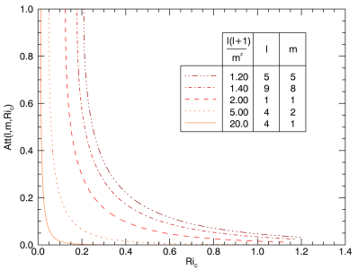
Figure 1: Attenuation rate Att=$e^{-\pi\sqrt{\frac{l(l+1)}{m^{2}}\mathrm{Ri}_{c}-\frac{1}{4}}}$ of the wave passing through a critical layer as a function of the Richardson number. We observe that Att increases with $\displaystyle\frac{l(l+1)}{m^{2}}$.

We have not yet discussed a latter point: the choice of the method of resolution. Most of the publications concerning IGWs use another process to solve the equation of propagation (Press, 1981; Zahn et al., 1997; Mathis, 2009). In fact, the WKBJ theory is particularly adapted to the resolution of this equation. However, it is not convenient in our case because it imposes a condition on the value of the Richardson number as demonstrated in appendix A. It is shown that the WKBJ approximation is available only if $\mathrm{Ri}_{c}\gg\frac{1}{4}\frac{m^{2}}{l(l+1)}$. Despite this restriction, let us write the solution. By separating the domain into two parts, we obtain

$$\Psi^{\rm WKBJ}_{l,m\pm}=\frac{1}{\sqrt{k_{V}(r)}}(C_{\pm}e^{i\int{k_{V}(r)dr}}+D_{\pm}e^{-i\int{k_{V}(r)dr}})\hbox{.}$$ (34)

As

$$k_{V}\underset{\mathrm{Ri}_{c}\gg\frac{1}{4}\frac{m^{2}}{l(l+1)}}{\longrightarrow}\frac{1}{r-r_{c}}\sqrt{\frac{l(l+1)}{m^{2}}\mathrm{Ri}_{c}}\hbox{,}$$ (35)

it comes :

$$\Psi^{\rm WKBJ}_{l,m\pm}=\frac{m}{\sqrt{l(l+1)}\mathrm{Ri}_{c}}(r-r_{c})^{1/2}\left(C_{\pm}(r-r_{c})^{+i\sqrt{\frac{l(l+1)}{m^{2}}\mathrm{Ri}_{c}}}\right.$$ (36)

$$\left.+D_{\pm}(r-r_{c})^{-i\sqrt{\frac{l(l+1)}{m^{2}}\mathrm{Ri}_{c}}}\right)\hbox{.}$$ (37)

It is comforting to see that both methods (Frobenius and WKBJ) give the same solution, to a multiplicative constant, when the Richardson number become high:

$$\Psi^{\rm Fro}_{l,m}\underset{\mathrm{Ri}_{c}\gg\frac{1}{4}\frac{m^{2}}{l(l+1)}}{\longrightarrow}\Psi^{\rm WKBJ}_{l,m}\hbox{.}$$ (38)

3.4 The unstable case: $\mathrm{Ri}_{c}<\frac{1}{4}\frac{m^{2}}{l(l+1)}$

In the unstable regime, the Frobenius method also gives a solution but we are not able to indentify upward and downward propagating waves because of shear-induced instability and turbulence. As a consequence we can not connect the solutions at the critical layer. In order to avoid this difficulty, we here propose to solve Eq. (21) following the method developped by Lindzen & Barker (1985). They applied it in the case of cartesian coordinates and our bringing is to generalize it to spherical coordinates. The parameter $\eta_{l,m}$ defined in Eq. (25) is real in this case and we introduce

$$X=k_{Hc}(r-r_{c})\hbox{.}$$ (39)

Equation (21) becomes:

$$\frac{\mathrm{d}^{2}\Psi_{l,m}(X)}{\mathrm{d}X^{2}}+\left(\frac{\frac{1}{4}-\eta_{l,m}^{2}}{X^{2}}-1\right)\Psi_{l,m}(X)=0\hbox{.}$$ (40)

We are seeking solutions of the form $\Psi_{l,m}(X)=X^{\frac{1}{2}}\Phi_{l,m}(X)$, where $\Phi_{l,m}$ is the solution to the Bessel equation

$$X^{2}\frac{\mathrm{d}^{2}}{\mathrm{d}X^{2}}\Phi_{l,m}+X\frac{\mathrm{d}}{\mathrm{d}X}\Phi_{l,m}-(\eta_{l,m}^{2}+X^{2})\Phi_{l,m}=0\hbox{.}$$ (41)

Consequently, $\Phi_{l,m}$ is a combination of the Bessel’s modified functions $I_{\eta_{l,m}}(X)$ and $I_{-\eta_{l,m}}(X)$:

$$\Phi_{l,m}=K_{1}I_{\eta_{l,m}}(X)+K_{2}I_{-\eta_{l,m}}(X)\hbox{.}$$ (42)

The final solution is given by:

$$\Psi_{l,m}(X)=X^{\frac{1}{2}}\left(K_{1}I_{\eta_{l,m}}(X)+K_{2}I_{-\eta_{l,m}}(X)\right)\hbox{.}$$ (43)

We would like to calculate the reflection and transmission coefficients of the wave passing through the unstable critical layer. We assume that the fluid has the profile described in Fig. 2. We decompose the studied region into three zones defined by the value of the quantity $\frac{l(l+1)}{m^{2}}\mathrm{Ri}_{c}$. In zones I and III, the Richardson number is high enough to allow us to apply the WKBJ method described in the previous part. In unstable zone II around the studied critical layer however, we must use the solution with the modified Bessel functions. Moreover, we assume here that the thickness $2\delta$ of this latter is small in comparison with the characteristic length of the problem. Then, we can consider that the wavenumber $k_{V}$ is constant as

$$k_{Vc}^{2}=\frac{l(l+1)}{m^{2}}\frac{\mathrm{Ri}_{c}}{\delta^{2}}-\frac{l(l+1)}{r_{c}^{2}}\hbox{.}$$ (44)

Let us consider a wave coming from the overside of the critical layer (zone I). It is partly transmitted toward zone III and partly reflected backward zone I. We so write the solutions corresponding to the three zones:

$$\left\{\begin{array}[]{l}\Psi_{I}(r)=e^{-ik_{V}(r-r_{c})}+Re^{ik_{V}(r-r_{c})}\hbox{,}\\ \Psi_{II}(r)=(r-r_{c})^{1/2}\left[AI_{\eta_{l,m}}(k_{Hc}(r-r_{c}))+BI_{-\eta_{l,m}}(k_{Hc}(r-r_{c}))\right]\hbox{,}\\ \Psi_{III}(r)=Te^{ik_{V}(r-r_{c})}\hbox{,}\end{array}\right.$$ (45)

where $\Psi_{I}(r)$ is available if $(r-r_{c})>\delta$, $\Psi_{II}(r)$ if $-\delta<(r-r_{c})<\delta$ and $\Psi_{III}(r)$ if $(r-r_{c})>-\delta$. The coefficients $A$, $B$, $T$ and $R$ are calculated thanks to the following four continuity equations:

$$\left\{\begin{array}[]{l}\Psi_{I}(r_{c}+\delta)=\Psi_{II}(r_{c}+\delta)\hbox{,}\\ \displaystyle\frac{\mathrm{d}\Psi_{I}}{\mathrm{d}r}(r_{c}+\delta)=\displaystyle\frac{\mathrm{d}\Psi_{II}}{\mathrm{d}r}(r_{c}+\delta)\hbox{,}\\ \Psi_{III}(r_{c}-\delta)=\Psi_{II}(r_{c}-\delta)\hbox{,}\\ \displaystyle\frac{\mathrm{d}\Psi_{III}}{\mathrm{d}r}(r_{c}-\delta)=\displaystyle\frac{\mathrm{d}\Psi_{II}}{\mathrm{d}r}(r_{c}-\delta)\hbox{.}\end{array}\right.$$ (46)

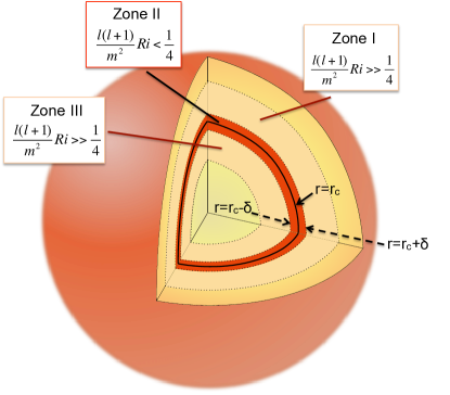
Figure 2: Assumed neighbourhood of an unstable critical layer for the calculation of the IGWs’ reflection and transmission coefficients. We assume that the unstable region around the critical layer (in red) has a thickness given by $2\delta$ (Zone II). The surrounding regions where IGWs are propagative are in beige (Zones I and III).

They correspond to the continuity of the solution and of its first derivative, which physically means that both displacement and mechanical stresses are continuous. After some algebra, we obtain the coefficients $R$ and $T$ of reflection and transmission, depending on the stiffness $\delta$, on the vertical and horizontal wavenumbers $k_{Vc}$ and $k_{Hc}$ (see Eq. (44) and (23)) , and on the variable $\eta_{l,m}$ (Eq. (25)). In order to lighten the formula, we note $I_{\pm\eta_{l,m}}$ instead of $I_{\pm\eta_{l,m}}(k_{Hc}\delta)$. Then, we obtain

$$R=\frac{R_{\mathrm{num}}}{R_{\mathrm{denom1}}+R_{\mathrm{denom2}}}\hbox{,}$$ (47)

with

$$R_{\mathrm{num}}\!=\!\left[k_{Hc}I_{\eta_{l,m}}^{\prime}+\left(\frac{1}{2\delta}-ik_{Vc}\right)I_{\eta_{l,m}}\right]\!\left[k_{Hc}I_{-\eta_{l,m}}^{\prime}+\left(\frac{1}{2\delta}-ik_{Vc}\right)I_{-\eta_{l,m}}\right]\!\hbox{,}$$

$$R_{\mathrm{denom1}}=k_{Hc}^{2}I_{-\eta_{l,m}}^{\prime}I_{-\eta_{l,m}}+\left(\frac{1}{4\delta^{2}}+k_{Vc}^{2}\right)I_{-\eta_{l,m}}I_{\eta_{l,m}}\hbox{,}$$

$$R_{\mathrm{denom2}}=-\frac{2k_{Vc}}{\pi\delta}\cos\left(\eta_{l,m}\pi\right)+\frac{k_{Hc}}{2\delta}\left(I_{\eta_{l,m}}I_{-\eta_{l,m}}^{\prime}+I_{-\eta_{l,m}}I_{\eta_{l,m}}^{\prime}\right)$$

and

$$T=\frac{T_{\mathrm{num}}}{T_{\mathrm{denom}}}\hbox{,}$$ (48)

with

$$T_{\mathrm{num}}=\frac{2ik_{Vc}}{\delta\pi}\hbox{,}$$

$$T_{\mathrm{denom}}=R_{\mathrm{denom1}}+R_{\mathrm{denom2}}\hbox{.}$$

We have now calculated the transmission and reflection coefficients of an IGW, under some assumption, through an unstable region around a given critical layer where $\mathrm{Ri}_{c}<\frac{1}{4}\frac{m^{2}}{l(l+1)}$. We represent the level lines of $|R|$ and $|T|$ in Fig. 3 for $l=4$ and $m=\pm 3$. They are plotted as function of the Richardson number at the critical layer $\mathrm{Ri}_{c}$, growing from 0 to its maximum value defined by $\frac{l(l+1)}{m^{2}}{\mathrm{Ri}_{c}}_{max}=\frac{1}{4}$. For instance, in Fig. 3, ${\mathrm{Ri}_{c}}_{max}=\frac{1}{4}\frac{3^{2}}{4(4+1)}\approx 0.11$. The other variable is the half-thickness $\delta$ of the unstable layer (zone II), arbitrarily choosen, that points the non-local character of unstable turbulent layers. Let us underline the main result: both coefficients are greater than 1 when $\frac{l(l+1)}{m^{2}}\mathrm{Ri}_{c}$ is small enough. Consequently, for a low Richardson number at the critical layer, the wave can be over-reflected and over-transmitted at the same time. It means that on the contrary of the first stable case, the wave take potential energy from the unstable fluid and convert it into kinetic energy. In other words, the turbulent layer acts as an excitation region. If $|R|<1$ and $|T|<1$, we speak about IGWs ”tunneling” (Sutherland & Yewchuk, 2004; Brown & Sutherland, 2007; Nault & Sutherland, 2007). Another remark concerns de dependency of $|R|$ and $|T|$ with $m$. We denote that the sign of $m$ does not matter since only its square appears in the expressions. Physically, it shows that the critical layer’s action is the same on prograde and retrograde waves. This point is of importance because we know that other dissipative processes occuring during the propagation of IGW discriminate between both types of waves.

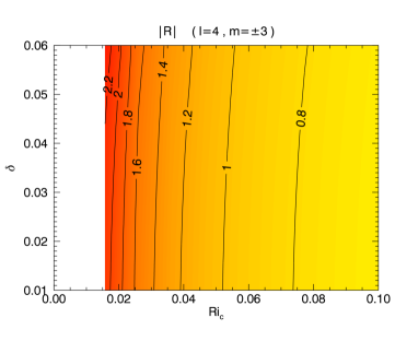
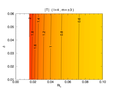
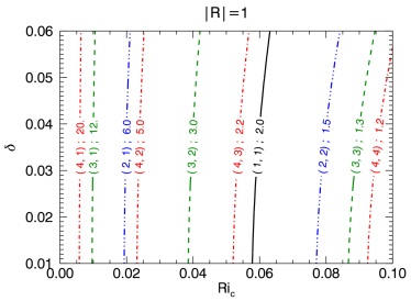
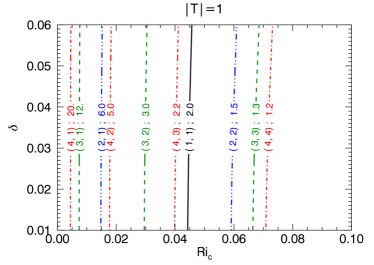
Figure 3: Level lines of reflection $|R|$ and transmission $|T|$ coefficients of an IGW at a critical layer as a function of the Richardson number $\mathrm{Ri}_{c}$ and of the thickness $\delta$ of the critical layer (zone II in Fig. 2). The top panels represent the level lines for an arbitrary choosen value of $(l,m)=(4,\pm 3)$, while the bottom panels show levels lines $|R|=1$ and $|T|=1$ for different couples $(l,m)$.

In order to visualize the action of the critical layer on differents waves, Fig. 2 shows the level lines $|R|=1$ for $1\leq l\leq 5$ and $1\leq m\leq l$. We previously said that it is useless to consider negative values of $m$ since $|R|$ depends only on $m^{2}$. The pair ($l$,$m$) is indicated on each ligne, followed by the value of $\frac{l(l+1)}{m^{2}}$. Lines in the same color correspond to the same value of $l$. These lines mark out the limit to observe over-reflection, for a chosen wave. We observe that higher is the value of $\frac{l(l+1)}{m^{2}}$, stronger is the condition on $\mathrm{Ri}_{c}$ to observe an over-reflection.

3.5 Choice of the method

We have decided to apply different methods to solve the stable and unstable cases. However, it could be legitimate to wonder if both methods are equivalent from a mathematical point of view. In this part, we present a short comparison between the solutions obtained with the method of Frobenius and the one with Bessel functions. The modified Bessel function $I_{\eta_{l,m}}(X)$ can be computed using

$$I_{\eta_{l,m}}(X)=\left(\frac{1}{2}X\right)^{\eta_{l,m}}\sum\limits_{k=0}^{\infty}\frac{\left(\frac{1}{2}X\right)^{2k}}{k!\Gamma(\eta_{l,m}+k+1)}\hbox{.}$$ (49)

At the neighbourhood of the critical layer, X tends to $0$ and the first-order expression is

$$I_{\eta_{l,m}}(X)=\left(\frac{1}{2}X\right)^{\eta_{l,m}}\left(\frac{1}{\Gamma(\eta_{l,m}+1)}+O(X^{2})\right)\hbox{.}$$ (50)

Close to the critical layer, the global solution given in Eq. (43) is then

$$\Psi_{l,m}^{\rm Bessel}(X)=\left(\Delta_{1}\frac{X^{\frac{1}{2}+\eta_{l,m}}}{\Gamma(\eta_{l,m}+1)}+\Delta_{2}\frac{X^{\frac{1}{2}-\eta_{l,m}}}{\Gamma(1-\eta_{l,m})}+O(X^{2})\right)\hbox{.}$$ (51)

Now, let us remind the expression of the solution given by the method of Frobenius (Eq. (26)), rewritten with the previous notations

$$\Psi_{l,m}^{\rm Fro}(r)=A_{2}|r-r_{c}|^{1/2+\eta_{l,m}}+B_{2}|r-r_{c}|^{1/2-\eta_{l,m}}.$$

In conclusion, for a fixed couple $(l,m)$, $\Psi_{l,m}^{\rm Fro}(r)$ and $\Psi_{l,m}^{\rm Bessel}(X)$ vary in the same way as function of $r-r_{c}$.

4 Case of the non-perfect fluid

From now, we have studied the role of the critical layers assuming that the fluid was perfect. In order to make the problem more realistic we include in the second part the viscosity $\nu$ of the fluid and the coefficient of thermal conductivity $\kappa$ (e.g. Koppel, 1964; Hazel, 1967; Baldwin & Roberts, 1970; Van Duin & Kelder, 1986).

4.1 Equation of propagation of IGW near a critical layer

The linearized equations of hydrodynamics in Eq. (6) become:

$$\left\{\begin{array}[]{l}D_{t}\@vec{u}=-\frac{\@vec{\nabla}p^{\prime}}{\bar{\rho}}+\frac{\rho^{\prime}}{\bar{\rho}}\@vec{g}+\nu\Delta\@vec{u}\hbox{,}\\ D_{t}\rho^{\prime}+\@vec{\nabla}.(\bar{\rho}\@vec{u})=0\hbox{,}\\ D_{t}\left(\frac{\rho^{\prime}}{\bar{\rho}}-\frac{1}{\Gamma_{1}}\frac{p^{\prime}}{\bar{p}}\right)-\frac{N^{2}}{g}u_{r}=\frac{\kappa}{\bar{\rho}}\Delta\rho^{\prime}\hbox{.}\end{array}\right.$$ (52)

The following method for the building of the propagation equation is adapted from the work of Baldwin & Roberts (1970). We assume that the mean density $\bar{\rho}$ of the fluid nearly takes a constant value, that is to say that $\frac{1}{\bar{\rho}}\frac{\mathrm{d}\bar{\rho}}{\mathrm{d}r}$ is small compared with others characteristic lenghts. First, we project Eq. (52) onto $\hat{e}_{r}$ and apply the operator $\@vec{\nabla}^{2}$. Then we apply $D_{t}-\kappa\@vec{\nabla}^{2}$. After combination with the two other equations, we obtain :

$$(D_{t}-\kappa\@vec{\nabla}^{2})\left[(D_{t}-\nu\@vec{\nabla}^{2})(\@vec{\nabla}^{2}u_{r}+(\Omega^{\prime\prime}+\frac{2}{r}\Omega^{\prime})\partial_{\varphi}u_{r}\right]=N^{2}\@vec{\nabla}_{\perp}^{2}u_{r}\hbox{.}$$ (53)

As done in the previous part, we decompose the radial velocity on the basis of spherical harmonics

$$u_{r}(r,\theta,\varphi,t) = \sum\limits_{l,m}\hat{u}_{r;l,m}(r)Y_{l,m}(\theta,\varphi)e^{i\sigma_{w}t}\hbox{,}$$ (54)

where $\sigma=\sigma_{w}+m\Delta\Omega(r)$. Moreover, it is easier to work with dimensionless numbers. For this reason, we introduce the notations detailed in Tab. 1.

Table 1: Dimensionless numbers used for the resolution of Eq. (53). $L$ and $V$ are respectively the length and velocity scales.

$P_{\mathrm{r}}$	$\nu/\kappa$	Prandtl number
$R_{\mathrm{e}}$	$VL/\nu$	Reynolds number
$\mathrm{Ri}$	$\left(LN/V\right)^{2}$	Richardson number

Then, Eq. 53 becomes for each pair ($l$,$m$) such as $l\in\mathbb{N}$ and $m\in\llbracket-l,l\rrbracket$ :

$$\left(\Delta_{l}-k_{H}^{2}-i\sigma R_{\mathrm{e}}P_{\mathrm{r}}\right)\left(\Delta_{l}-k_{H}^{2}-i\sigma R_{\mathrm{e}}\right)\left(\Delta_{l}-k_{H}^{2}\right)\hat{u}_{r;l,m}$$

$$=-k_{H}^{2}R_{\mathrm{e}}^{2}P_{\mathrm{r}}N^{2}\hat{u}_{r;l,m}\hbox{,}$$ (55)

where $\Delta_{l}$ is the scalar spherical Laplacian operator :

$$\Delta_{l}=\partial_{rr}^{2}+\frac{2}{r}\partial_{r}-\frac{l(l+1)}{r^{2}}\hbox{.}$$ (56)

Lastly, we introduce $\eta=(im\Omega_{c}^{\prime}R_{\mathrm{e}})^{1/3}(r-r_{c})$ and thanks to a developpement close to the critical layer we obtain the sixth-order equation:

$$\frac{1}{P_{\mathrm{r}}}\frac{\partial^{6}\chi_{l,m}}{\partial\eta^{6}}-\eta\left(1+\frac{1}{P_{\mathrm{r}}}\right)\frac{\partial^{4}\chi_{l,m}}{\partial\eta^{4}}-\frac{2}{P_{\mathrm{r}}}\frac{\partial^{3}\chi_{l,m}}{\partial\eta^{3}}$$ (57)

$$+ \eta^{2}\frac{\partial^{2}\chi_{l,m}}{\partial\eta^{2}}+\frac{l(l+1)}{m^{2}}\mathrm{Ri}_{c}\chi_{l,m}=0\hbox{,}$$

where now $\chi_{l,m}=\bar{\rho}^{1/2}\eta\hat{u}_{\eta;l,m}$. Equation (57) can be compared with the one obtained by Press (1981) who has neglected the viscosity $\nu$. Moreover, we can see that if we take $\nu=\kappa=0$, and without forgetting that $P_{r}$ depends on $\nu$ too, Eq. (57) is identical to Eq. (21) for the perfect fluid.

4.2 Mathematical resolution

The resolution of Eq. (57) requests several substitutions and is quite complex. The detailed calculation can be found in appendix B and we give here only the main steps. We draw our inspiration from Hazel (1967); Baldwin & Roberts (1970); Koppel (1964); Van Duin & Kelder (1986) who solve the same equation in cartesian coordinates. However, the resolution in spherical coordinates has some differences. The aim is here to rewrite the equation under a known form: the Whittaker differential equation; then, after some algebra, we can show that Eq. (57) can be written in the following form

$$\frac{\mathrm{d}^{2}V}{\mathrm{d}s^{2}}+\left(\frac{\frac{1}{4}-M_{l,m}^{2}}{s^{2}}+\frac{\Lambda}{s}-\frac{1}{4}\right)V=0\hbox{.}$$ (58)

The solutions of Eq. (58) are thus the Whittaker functions (Abramowitz & Stegun, 1965):

$$V_{\Lambda,M_{l,m}}(s)=e^{-\frac{s}{2}}s^{\frac{1}{2}+M_{l,m}}{{}_{1}F_{1}}\left(\frac{1}{2}+M_{l,m}+\Lambda;1+2M_{l,m};s\right)\hbox{,}$$ (59)

where ${}_{1}F_{1}$ is the confluent hypergeometric function of Kummer

$${}_{1}F_{1}(a;b;z)=\sum\limits_{n=0}^{\infty}\frac{(a)_{n}}{(b)_{n}}\frac{z^{n}}{n!}$$ (60)

with $(k)_{n}=\prod\limits_{i=0}^{n-1}(k+i)=\frac{\Gamma\left(k+n\right)}{\Gamma\left(k\right)}$ and $(k)_{0}=1$, $\Gamma\left(z\right)$ being the usual Gamma function,

$$M_{l,m}^{2}=\frac{1}{4}-\frac{2+\frac{l(l+1)}{m^{2}}\mathrm{Ri}_{c}}{9}\hbox{,}$$ (61)

and

$$\Lambda=-\frac{1}{3}\hbox{.}$$ (62)

Thanks to this solution, we obtain the expression of the radial displacement of the wave:

$$\bar{\rho}^{1/2}\eta^{2}\hbox to0.0pt{$\displaystyle\hat{\xi}_{\eta;l,m}\!\propto\!$\hss}$$

$$f(\kappa,P_{\rm r}) \int_{a}^{b} {e^{\eta t-t^{3}/3}t^{3M_{l,m}-3/2}{{}_{1}F_{1}}\left(\frac{1}{6}+M_{l,m};1+2M_{l,m};t\right)dt}\,\hbox{;}$$

we will clarify the function $f(\kappa,P_{\rm r})$ of the thermal diffusivity coefficient later.

There is still the last step to get over. We must find a curve along which we integrate the solution, that is to say, we determine $a$ and $b$. During the calculation detailed in the appendix B, Eq. (104):

$$\left[-\left(1+\frac{1}{P_{\mathrm{r}}}\right)t^{4}ve^{\eta t}-\frac{\mathrm{d}}{\mathrm{d}t}\left(t^{2}v\right)e^{\eta t}+zt^{2}ve^{\eta t}\right]_{a}^{b}=0$$ (64)

has not been used yet. A sufficient condition to make this egality true is $\frac{-t^{3}}{3}\underset{|t|\to+\infty}{\longrightarrow}\infty$. Considering that $t^{3}=|t|^{3}e^{3i\theta_{t}}$ ($\theta_{t}$ being the complex argument of $t$), we have

$$\frac{-t^{3}}{3}\underset{|t|\to+\infty}{\longrightarrow}\infty\hbox{ }\Leftrightarrow\hbox{ }\theta_{t}\equiv 0\left[\frac{2\pi}{3}\right]\hbox{.}$$ (65)

There are several possibilities for the choice of the curves. Koppel (1964) propose to build a basis of six solutions using the curves ($\mathcal{C}_{1}$,$\mathcal{C}_{2}$,$\mathcal{C}_{3}$) represented in Fig. 6 (left). Therefore, the solutions of the sixth order equation (Eq. (57)) are linear combinations of

$$U_{i}(\eta)=f(\kappa,P_{\rm r})$$ (66)

$$\times\int_{\mathcal{C}_{i}}{e^{\eta t-t^{3}/3}t^{3M_{l,m}-3/2}{{}_{1}F_{1}}\left(\frac{1}{6}M_{l,m};1+2M_{l,m};t\right)}\,\mathrm{d}t$$

and $V_{i}(\eta)$ with $i\in\{1,2,3\}$, where $V_{i}(\eta)$ corresponds to $U_{i}(\eta)$ with the opposite sign for $M_{l,m}$.

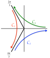
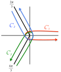
Figure 4: Left: curves ($\mathcal{C}_{1}$,$\mathcal{C}_{2}$,$\mathcal{C}_{3}$) defining the basis ($U_{1},U_{2},U_{3},V_{1},V_{2},V_{3}$). Right: curves ($\mathcal{C}^{\prime}_{1}$,$\mathcal{C}^{\prime}_{2}$,$\mathcal{C}^{\prime}_{3}$) defining the basis ($u_{1},u_{2},u_{3},v_{1},v_{2},v_{3}$).

4.3 Application to IGWs

It is now time to apply these mathematical results to IGWs. With this aim in view, let us remind the solution for the perfect fluid obtained in the first part. For the moment, it is not necessary to distinguish between the stable regime, i.e. $\frac{l(l+1)}{m^{2}}\mathrm{Ri}_{c}>\frac{1}{4}$, and the unstable one, i.e. $\frac{l(l+1)}{m^{2}}\mathrm{Ri}_{c}<\frac{1}{4}$. The Frobenius solution is available everywhere if we take $\eta_{l,m}=\sqrt{\frac{1}{4}-\frac{l(l+1)}{m^{2}}\mathrm{Ri}_{c}}$ as a complex number. Remembering that $\Psi_{l,m}(r)=\bar{\rho}^{\frac{1}{2}}r^{2}\hat{\xi}_{r;l,m}(r)$, the radial Lagrangian displacement is

$$\left\{\begin{array}[]{l}\hat{\xi}_{\mathrm{P}+}=\frac{1}{\bar{\rho}^{1/2}r^{2}}\left(A|r-r_{c}|^{1/2+i\alpha_{l,m}}+B|r-r_{c}|^{1/2-i\alpha_{l,m}}\right)\\ \hat{\xi}_{\mathrm{P}-}=\frac{1}{\bar{\rho}^{1/2}r^{2}}\left(-iAe^{\alpha_{l,m}\pi}|r-r_{c}|^{1/2+i\alpha_{l,m}}-iBe^{-\alpha_{l,m}\pi}|r-r_{c}|^{1/2-i\alpha_{l,m}}\right)\hbox{.}\end{array}\right.$$ (67)

In order to make the reading easier, we have removed the indices $r;l,m$. Indice $P$ designates the solution for the perfect fluid.

Concerning the solution for non-perfect fluids, Hazel (1967) proposes to use another basis of the solutions of Eq. (57). The curves ($\mathcal{C}^{\prime}_{1}$,$\mathcal{C}^{\prime}_{2}$,$\mathcal{C}^{\prime}_{3}$) are represented in Fig. 6. The new basis ($u_{1},u_{2},u_{3},v_{1},v_{2},v_{3}$) is defined by:

• $u_{1}=U_{1}+U_{2}+U_{3}$ and $v_{1}=V_{1}+V_{2}+V_{3}$,

• $u_{2}=U_{1}+U_{2}+U^{*}_{3}$ and $v_{2}=V_{1}+V_{2}+V^{*}_{3}$,

• $u_{3}=U_{1}+U^{*}_{2}+U_{3}$ and $v_{3}=V_{1}+V^{*}_{2}+V_{3}$,

where $X^{*}$ is the complex conjugate of $X$. Consequently, the solution for the non-perfect fluid (indice NP) can be written as :

$$\hat{\xi}_{\mathrm{NP}\pm}=\frac{1}{\bar{\rho}^{1/2}\eta^{2}}\sum\limits_{i=1}^{3}\left[\alpha_{i\pm}u_{i}\left(\eta\right)+\beta_{i\pm}v_{i}\left(\eta\right)\right]\hbox{.}$$ (68)

A relation between both solutions $\hat{\xi}_{\mathrm{P}\pm}$ and $\hat{\xi}_{\mathrm{NP}\pm}$ exists if we consider that the Reynolds number is great. In the case of the Sun (e.g. Brun & Zahn, 2006), the microscopic viscosity in the radiative zone is weak. For this reason, it is appropriate to consider that the Reynolds number $R_{\mathrm{e}}=\frac{VL}{\nu}$ is much greater than 1. This assuption leads to the relation

$$\hat{\xi}_{\mathrm{NP}\pm}\underset{R_{\mathrm{e}}\to+\infty}{\longrightarrow}\hat{\xi}_{\mathrm{P}\pm}\hbox{.}$$ (69)

Baldwin & Roberts (1970) give tables for the asymptotic comportement of $u_{i}$ and $v_{i}$ ( i$\in{1,2,3}$). The solutions $u_{1}$, $u_{2}$, $v_{1}$ et $v_{2}$ diverge when $R_{\mathrm{e}}\to+\infty$. They are therefore physically unacceptable and we deduce that

$$\hat{\xi}_{\mathrm{NP}\pm}=\frac{1}{\bar{\rho}^{1/2}\eta^{2}}\alpha_{3\pm}u_{3}(\eta)+\beta_{3\pm}v_{3}(\eta)\hbox{.}$$ (70)

Tables (3) and (3) give the asymptotic expressions of $u_{3}$ and $v_{3}$ as a function of the sign of $r-r_{c}$.

Table 2: Expressions of $u_{3}$ and $v_{3}$ when $R_{\mathrm{e}}\to+\infty$, below the critical layer.

$r>r_{c}$
$u_{3}(\eta)$	$\displaystyle\frac{2i\pi}{\Gamma(\frac{3}{2}-i\alpha_{l,m})}(im\Omega_{c}^{\prime}R_{\mathrm{e}})^{\frac{1}{3}\left(\frac{1}{2}-i\alpha_{l,m}\right)}|r-r_{c}|^{\frac{1}{2}-i\alpha_{l,m}}$
$v_{3}(\eta)$	$\displaystyle\frac{2i\pi}{\Gamma(\frac{3}{2}+i\alpha_{l,m})}(im\Omega_{c}^{\prime}R_{\mathrm{e}})^{\frac{1}{3}\left(\frac{1}{2}+i\alpha_{l,m}\right)}|r-r_{c}|^{\frac{1}{2}+i\alpha_{l,m}}$

Table 3: Expressions of $u_{3}$ and $v_{3}$ when $R_{\mathrm{e}}\to+\infty$, above the critical layer.

$r<r_{c}$
$u_{3}(\eta)$	$\displaystyle\frac{2\pi}{\Gamma(\frac{3}{2}-i\alpha_{l,m})}e^{-\alpha_{l,m}\pi}(im\Omega_{c}^{\prime}R_{\mathrm{e}})^{\frac{1}{3}\left(\frac{1}{2}-i\alpha_{l,m}\right)}|r-r_{c}|^{\frac{1}{2}-i\alpha_{l,m}}$
$v_{3}(\eta)$	$\displaystyle\frac{2\pi}{\Gamma(\frac{3}{2}+i\alpha_{l,m})}e^{-\alpha_{l,m}\pi}(im\Omega_{c}^{\prime}R_{\mathrm{e}})^{\frac{1}{3}\left(\frac{1}{2}+i\alpha_{l,m}\right)}|r-r_{c}|^{\frac{1}{2}+i\alpha_{l,m}}$

In the stable case where $\frac{l(l+1)}{m^{2}}\mathrm{Ri}_{c}\geq\frac{1}{4}$, $\alpha_{l,m}=\sqrt{\frac{l(l+1)}{m^{2}}\mathrm{Ri}_{c}-\frac{1}{4}}$ is a real number. The same findings than in the previous part can be made: after the passage through the critical layer, the wave is attenuated by a factor $e^{-\alpha_{l,m}\pi}$. In the unstable case where $\frac{l(l+1)}{m^{2}}\mathrm{Ri}_{c}<\frac{1}{4}$, $\alpha_{l,m}=\sqrt{\frac{l(l+1)}{m^{2}}\mathrm{Ri}_{c}-\frac{1}{4}}$ is a complex number, so we can not interpret the solution as upward and downward propagating waves. But the expressions given in Tab. (3) and (3) remain comparable to those in the first part and we deduce that the calculation of $R$ and $T$ will lead to the same result: the possibility of over-reflection and over-transmission.

4.4 Radiative and viscous dampings

4.4.1 General equations

We volontary left aside the factor $f(\kappa,P_{\rm r})$ in Eq. (66). In order to establish its expression, Zahn et al. (1997) use the equation of IGWs propagation taking into account heat diffusion but with a viscosity coefficient ($\nu$) equals to zero. Here, we generalize their result for $\nu\neq 0$ (i.e. $P_{\rm r}\neq 0$) and we obtain

$$f\left(\kappa,P_{\rm r}\right)=\displaystyle e^{-\tau\left(\kappa,P_{\rm r}\right)/2}\hbox{,}$$ (71)

where

$$\tau\left(\kappa,P_{\rm r}\right)=\left[l(l+1)\right]^{\frac{3}{2}}\int_{r_{c}}^{r_{\rm ZC}}\left\{\kappa\left(1+P_{\rm r}\right)\frac{NN_{T}^{2}}{\sigma^{4}}\left(\frac{N^{2}}{N^{2}-\sigma^{2}}\right)^{\frac{1}{2}}\frac{1}{r^{3}}\right\}\mathrm{d}r\hbox{.}$$ (72)

We have introduced the general expression for $N^{2}$, the Brünt-Väisälä frequency, to be able to take into account chemical stratification. Then, we have

$$N^{2}=N_{T}^{2}+N_{\mu}^{2}$$ (73)

with $N_{T}^{2}=\frac{{\overline{g}}\delta}{H_{P}}\left(\nabla_{\rm ad}-\nabla\right)$ and $N_{\mu}^{2}=\frac{{\overline{g}}\phi}{H_{P}}\nabla_{\mu}$ where $H_{P}=|{\rm d}r/{\rm d}\ln{\overline{P}}|$ is the pressure height-scale, $\nabla=\left({\partial\ln{\overline{T}}}/{\partial\ln{\overline{P}}}\right)$ the temperature gradient and $\nabla_{\mu}=\left(\partial\ln{\overline{\mu}}/\partial\ln{\overline{P}}\right)$ the mean molecular weight ($\mu$) gradient. Moreover, we have introduced the generalized equation of state (EOS) given in Kippenhahn & Weigert (1990):

$$\frac{{\rm d}\rho}{\rho}=\frac{1}{\Gamma_{1}}\frac{{\rm d}P}{P}-\tilde{\delta}\frac{{\rm d}T}{T}+\tilde{\phi}\frac{{\rm d}\mu}{\mu}\,,$$ (74)

where $\tilde{\delta}=-\left(\partial\ln\rho/\partial\ln T\right)_{P,\,\mu}$ and $\tilde{\phi}=\left(\partial\ln\rho/\partial\ln\mu\right)_{P,\,T}$. Next, $\sigma=\sigma_{w}+m\Delta\Omega$ is the Doppler-shifted frequency of the wave relative to the fluid rotation with an excitation frequency $\sigma_{w}$. $r_{c}$ and $r_{\rm CZ}$ are respectively the positions of the critical layer and of the boundary between the studied radiative zone and the convection region where IGWs are initially excited. This damping is another source of attenuation independent from the presence of a critical layer. Moreover, as shown in §3.4. and §4., we will have to consider IGWs reflected and transmitted by unstable critical layers in addition to those initially excited by convection. Then, we introduce the following notation

$$\tau\left[\kappa,P_{\rm r},r_{1},r_{2}\right]=$$ (75)

$$\left[l(l+1)\right]^{\frac{3}{2}}\int_{r_{2}}^{r_{1}}\left\{\kappa\left(1+P_{\rm r}\right)\frac{NN_{T}^{2}}{\sigma^{4}}\left(\frac{N^{2}}{N^{2}-\sigma^{2}}\right)^{\frac{1}{2}}\frac{1}{r^{3}}\right\}\mathrm{d}r\hbox{,}$$

where $r_{1}$ and $r_{2}$ are respectively the studied IGW’s emission point and the studied position with $r_{1}>r_{2}$ (in the opposite case where $r_{1}<r_{2}$, limits in the integral have to be reversed). This will enable us to describe radiative and viscous dampings in every configuration. Note that in stellar radiation zones $P_{\rm r}\!<\!\!<\!1$ (Brun & Zahn, 2006) inducing that the damping is mostly radiative. We have now to compare it with critical layers’ effects.

4.4.2 Progrades and retrogrades waves

For a same environnement, prograde waves have a frequency lower than retrograde ones (e.g. Eq. 4). We choose for example a couple of IGWs with the same excitation frequency, $\sigma_{0}$, same number $l$ and opposite azimuthal degree $m$. Thus, we compare a prograde wave of frequency $\sigma_{1}(r)=\sigma_{0}-|m|\Delta\Omega$ and a retrograde one of frequency $\sigma_{2}(r)=\sigma_{0}+|m|\Delta\Omega$. We obtain $\sigma_{1}(r)-\sigma_{2}(r)=-2|m|\left(\Omega(r)-\Omega_{\text{CZ}}\right)<0$ in the presence of negative gradient of $\Omega$ and $\sigma_{1}(r)-\sigma_{2}(r)>0$ if the gradient is positive. Now, let us underline that $\tau$ given in Eq. (71) varies globaly as $\frac{1}{\sigma^{3}}$. As a consequence, assuming that a negative $\Omega$-gradient is present near the excitation layer (see §. 6), the radiative damping is stronger for prograde waves than retrograde waves. Therefore, prograde IGWs are absorbed by the fluid much closer to their region of excitation while the retrograde waves are damped in a deeper region. This process is responsible for the net transport of angular momentum by IGWs in stars. On the other hand, critical layers doesnt introduce such net bias between prograde and retrgrade IGWs because their effects scale with $m^{2}$.

4.4.3 Dependency in $l$ and $m$

The second remark concerns the variation of radiative and viscous dampings as a function of $l$ and $m$. On one hand, looking at the multiplicative factor, which is in front of the integral in Eq. (72), we can roughly write that $\tau\propto{\frac{\left[l\left(l+1\right)\right]^{3/2}}{m^{4}}}$. On the other hand, the expression of the attenuation factor due to stable critical layers is proportional to $\left(\frac{l(l+1)}{m^{2}}\right)^{1/2}$, which is always greater than unity since $|m|\leq l$. The comparison between radiative and viscous dampings and the one due to stable critical layers for an IGW with given $\left(l,m\right)$ will be examined in §6.2.3.

4.4.4 Location

Lastly, radiative and viscous dampings occur throughout the whole propagation of IGWs. On the contrary, critical layers are localised. Moreover, there is a condition for a wave to reach a critical layer: the rotation speed of the fluid must be of the same order than the wave frequency to hope observing $\sigma=0$. Finally, all IGWs are concerned by radiative and viscous dampings, which increase around critical layers since $\tau\propto\sigma^{-4}$.

In Tab. (4), we sum up the different cases studied in these work. Depending on both properties of the fluid and of the studied wave, these latter is submitted to different phenomena.

Table 4: Summary of the different studied cases. The observed effects depend on the properties of the wave (the frequency ($\sigma$) and degrees ($l$, $m$)) and of the fluid (thermal conductivity ($\kappa$), viscosity coefficient ($\nu$), Richardson number ($\mathrm{Ri}$)).

wave and fluid properties
$\sigma(r_{c})$	$\kappa$	$\nu$	$\frac{l(l+1)}{m^{2}}\mathrm{Ri}_{c}$
$\neq 0$	not a critical layer
0	0	0	$\geq 1/4$	attenuation	Fig. 1
			$<1/4$	possible over-reflection + possible over-transmission	Fig. 3
	$\neq 0$
		$\ll 1$	$\geq 1/4$	attenuation + radiative damping
		$\ll 1$	$<1/4$	possible over-reflection + possible over-transmission + radiative damping
		$\gg 1$	non stellar case

5 Transport of angular momentum

As emphasized in the introduction, our goal is to study the transport of angular momentum in stellar radiation zones and to unravel the role of critical layers. Therefore, the first step is to recall the flux of angular momentum transported by propagative IGWs and by the shear-induced turbulence. Moreover, to illustrate our purpose, we will here focus on the case of a low-mass star where IGWs are initially excited at the border of the upper convective envelope (see Fig. 5) by turbulent convection (Garcia Lopez & Spruit, 1991; Dintrans et al., 2005; Rogers & Glatzmaier, 2005; Belkacem et al., 2009; Brun et al., 2011; Lecoanet & Quataert, 2012) and by tides if there is a close companion (Zahn, 1975; Ogilvie & Lin, 2007) with an amplitude $A$ (corresponding results for massive stars with an internal convective core can be easily deduced by reversing signs).

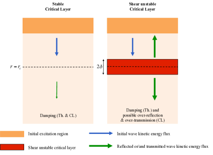
Figure 5: The two studied configurations in a low-mass star with an external convective envelope. Left: the case of a stable critical layer (CL) where IGWs are damped. Right: the case of an unstable critical layer where IGWs can be over-reflected/transmitted.

5.1 Angular momentum fluxes

5.1.1 Angular momentum flux transported by propagative IGWs

First, we have to calculate the angular momentum flux transported by a propagative monochromatic wave over a spherical surface. It is given by the horizontal average of the Reynolds stresses associated to the wave (e.g. Zahn et al., 1997):

$$\mathcal{F}_{J;l,m,\sigma}\left(r\right)=\bar{\rho}r\sin{\theta}<u_{r;l,m}u_{\varphi;l,m}>_{\theta,\varphi}\hbox{,}$$ (76)

where $<...>_{\theta,\varphi}=\displaystyle\frac{1}{4\pi}\int_{\Omega}...\sin\theta\mathrm{d}\theta\mathrm{d}\varphi$. Besides, Mathis (2009) shows that

$$\mathcal{F}_{J;l,m,\sigma}=\frac{-m}{\sigma}\mathcal{F}_{E;l,m,\sigma}\left(r\right)\hbox{,}$$ (77)

where $\mathcal{F}_{E;l,m,\sigma}$ is the horizontal average of the energy flux in the vertical direction expressed by Lighthill (1986) as

$$\mathcal{F}_{E;l,m,\sigma}=<\hat{p}^{\prime}_{l,m}u_{r;l,m}>_{\theta,\varphi}\hbox{.}$$ (78)

So finally, the angular momentum flux is given by

$$\mathcal{F}_{J;l,m,\sigma}=\frac{-m}{\sigma}<\hat{p}^{\prime}_{l,m}u_{r;l,m}>_{\theta,\varphi}\hbox{.}$$ (79)

To calculate this angular momentum flux, we need the expressions of $u_{r;l,m}$ and $\hat{p}^{\prime}_{l,m}$. $u_{r;l,m}$ is immediately accessible from Eq. (33), solution of Eq. (21). It is a little more complicated for $\hat{p}^{\prime}_{l,m}$ because we need to go back in the calculation leading to Eq. (21). The expression of $\hat{p}^{\prime}_{l,m}$ results from the first equation of the system given in Eq. (15), which can be reduced to

$$\frac{\mathrm{d}}{\mathrm{d}r}\left(\frac{\hat{p}^{\prime}_{l,m}}{\bar{\rho}}\right)=\left(\sigma^{2}-N^{2}\right)\hat{\xi}_{r;l,m}\hbox{,}$$ (80)

applying the anelastic approximation and neglecting terms of order $1/L^{2}$.

The total vertical flux of angular momentum transported by propagative IGWs is then given by

$${\mathcal{F}}_{J}\left(r\right)=\sum\limits_{l,m,\sigma}\mathcal{F}_{J;l,m,\sigma}$$ (81)

and we define the associated so-called action of angular momentum

$${\cal{L}}_{J}(r)=4\pi r^{2}{\mathcal{F}}_{J}\hbox{.}$$ (82)

5.1.2 Angular momentum flux transported by shear-induced turbulence

In the case of shear-unstable regions, such as region II in the regime where $\mathrm{Ri}_{c}\geq\frac{1}{4}\frac{m^{2}}{l\left(l+1\right)}$, IGWs are unstable (e.g. Drazin & Reid, 2004). After the non-linear saturation of the instability, a steady turbulent state is reached. Then, as established for example in Zahn (1992); Talon & Zahn (1997), and now confirmed by numerical simulations (see Prat & Lignières, 2013), the vertical flux of angular momentum transported by shear-induced turbulence is given by

$${\mathcal{F}}_{T;V}\left(r\right)={\overline{\rho}r^{2}\nu_{V}\left(r\right)\partial_{r}{\overline{\Omega}}},$$ (83)

where

$$\nu_{V}={{\rm Ri}^{\rm c}\over N^{2}_{T}/(\kappa+\nu_{H})+N^{2}_{\mu}/\nu_{H}}\left(r\partial_{r}\overline{\Omega}\right)^{2}\,.$$ (84)

${\rm Ri}^{\rm c}=1/6$ is the adopted value for the critical Richardson number and $\nu_{H}$ is the horizontal turbulent viscosity for which we assume the prescription derived by Zahn (1992).

5.1.3 Equation of transport of angular momentum

Let us now refocus these results in the wider frame of the complete angular momentum transport theory. Considering the other transport mechanisms we presented in introduction, the angular momentum transport equation taking into account meridional flows, shear-induced turbulence and IGWs (e.g. Talon & Charbonnel, 2005; Mathis, 2009) becomes

$${\overline{\rho}}\frac{\mathrm{d}}{\mathrm{d}t}\left(r^{2}{\overline{\Omega}}\right) = \frac{1}{5r^{2}}\partial_{r}\left({\overline{\rho}}r^{4}{\overline{\Omega}}U_{2}\left(r\right)\right)$$ (85)

$$+\begin{cases}-\displaystyle\frac{1}{4\pi r^{2}}\partial_{r}{\cal{L}}_{J}\left(r\right)\hbox{where IGWs are propagative}\\ \hbox{}\\ \displaystyle\frac{1}{r^{2}}\partial_{r}\left(r^{2}{\mathcal{F}}_{T;V}\left(r\right)\right)\hbox{for unstable regions.}\\ \end{cases}$$

The first term in the right hand side corresponds to the advection of angular momentum by the meridional circulation, where $U_{r}=U_{2}\,P_{2}(\cos\theta)$ is its radial component. $\frac{\mathrm{d}}{\mathrm{d}t}=\frac{\partial}{\partial t}+\dot{r}\frac{\partial}{\partial r}$ is the Lagrangian derivative that takes into account the radial contractions and dilatations of the star during its evolution, which are described by $\dot{r}\@vec{\hat{e}}_{r}$. According to our hypothesis, we do not take into account the transport by the Lorentz force, associated with magnetic fields in stellar radiative zones (Mathis & Zahn, 2005).

The major difference with previously published equations is that IGWs and shear-induced turbulence transports of angular momentum are not summed linearly since they are, as we demonstrated before, intrisically coupled. Therefore, for stable regions, one must take into account IGWs’ Reynolds stresses (Eq. 82) only, while for unstable regions, only the vertical turbulent flux given in Eq. (90) must be taken into account. Let us now examine each case of critical layer.

5.2 Stable critical layer $\left(\mathrm{Ri}_{c}\geq\displaystyle\frac{1}{4}\frac{m^{2}}{l\left(l+1\right)}\right)$

5.2.1 Case of the perfect fluid

This is the simplest case of a stable critical layer in a perfect fluid. Then, we apply Eq. (79) to obtain the expressions for the transported fluxes by propagative IGWs below and above the critical layer:

$$\left\{\begin{array}[]{l}\mathcal{F}_{J;l,m,\sigma}\left(r\geq r_{c}\right)=\displaystyle\frac{1}{r^{2}}\frac{1}{2}mA^{2}\,\frac{{\mathcal{J}}_{l,m}}{l\left(l+1\right)}\\ \\ \mathcal{F}_{J;l,m,\sigma}\left(r<r_{c}\right)=\displaystyle\frac{1}{r^{2}}\frac{1}{2}mA^{2}\,\frac{{\mathcal{J}}_{l,m}}{l\left(l+1\right)}e^{\displaystyle-2\pi\alpha_{l,m}}\hbox{,}\end{array}\right.$$ (86)

where A is the initial amplitude of the IGW at $r=r_{\rm CZ}$, $\alpha_{l,m}=\sqrt{\frac{l(l+1)}{m^{2}}\mathrm{Ri}_{c}-\frac{1}{4}}$ (see Eq. (27)) and

$${\mathcal{J}}_{l,m}=<\left[{P}_{l}^{m}\left(\cos\theta\right)\right]^{2}>_{\theta}=\frac{1}{2}\int_{0}^{\pi}\left[{P}_{l}^{m}\left(\cos\theta\right)\right]^{2}\sin\theta{\rm d}\theta$$ (87)

$$= \frac{2}{2l+1}\frac{\left(l+|m|\right)!}{\left(l-|m|\right)!}\hbox{,}$$

where ${P}_{l}^{m}$ are the associated Legendre polynomials. Booker & Bretherton (1967) have obtained similar results in cartesian coordinates. Let us make two remarks about these expressions. First, we see the expected attenuation of the flux by a factor $e^{-2\pi\alpha_{l,m}}$ when the wave passes through the critical layer. Moreover, $\mathcal{F}_{J;l,m,\sigma\pm}$ depends on $m$ (and not on $m^{2}$). As a consequence, we recover the classical result that prograde waves ($m<0$) and retrograde ones ($m>0$) have opposite angular momentum flux (respectively a deposit and an extraction). Finally, the monochromatic action of angular momentum ${\cal{L}}_{J;l,m,\sigma}(r)=4\pi r^{2}{\mathcal{F}}_{J;l,m,\sigma}$ is constant in each region because of the absence of dissipation.

5.2.2 Case of the non-perfect fuid

We saw in the previous part that the solution of the equation of propagation in the case of a non-perfect fluid is similar to the one obtained for a perfect fluid. For this reason, we are allowed to apply the same method for the calculation of $\mathcal{F}_{J;l,m,\sigma}$ and we obtain

$$\left\{\begin{array}[]{l}\mathcal{F}_{J;l,m,\sigma}\left(r\geq r_{c}\right)=\\ \displaystyle\frac{1}{r^{2}}\frac{1}{2}mA^{2}\,\frac{{\mathcal{J}}_{l,m}}{l\left(l+1\right)}e^{\displaystyle-\tau\left[\kappa,P_{\rm r},r_{\rm CZ},r\right]}\\ \\ \mathcal{F}_{J;l,m,\sigma}\left(r<r_{c}\right)=\\ \displaystyle\frac{1}{r^{2}}\frac{1}{2}mA^{2}\,\frac{{\mathcal{J}}_{l,m}}{l\left(l+1\right)}e^{\displaystyle-2\pi\alpha_{l,m}}e^{\displaystyle-\tau\left[\kappa,P_{\rm r},r_{\rm CZ},r\right]}\hbox{.}\end{array}\right.$$ (88)

The difference with Eq. (86) comes from the introduction of radiative and viscous dampings (Eq. 75).

The conclusion is that, in the stable case, the attenuation due to the passage through a critical layer is added to dampings due to dissipation. This observation will lead us to simply implement the role of stable critical layers as an additional term in the damping coefficient.

5.3 Unstable critical layer $\left(\mathrm{Ri}_{c}\leq\displaystyle\frac{1}{4}\frac{m^{2}}{l\left(l+1\right)}\right)$

5.3.1 Region I: $r_{c}+\delta\leq r\leq r_{\rm CZ}$

Using the summary given in Fig. 5 for the unstable case and the obtained results for regions where IGWs are propagative (§5.2.2.), we obtain:

$$\mathcal{F}_{J;l,m,\sigma}\left(r_{c}+\delta\leq r\leq r_{\rm CZ}\right)=$$ (89)

$$\frac{1}{r^{2}}\frac{1}{2}mA^{2}\,\frac{{\mathcal{J}}_{l,m}}{l\left(l+1\right)}e^{\displaystyle-\tau\left[\kappa,P_{\rm r},r_{\rm CZ},r\right]}$$

$$+ \frac{1}{r^{2}}\frac{1}{2}m\left[A^{2}{|R|}^{2}e^{\displaystyle-\tau\left[\kappa,P_{\rm r},r_{\rm CZ},r_{c}+\delta\right]}\right]\,\frac{{\mathcal{J}}_{l,m}}{l\left(l+1\right)}$$

$$\times\,e^{\displaystyle-\tau\left[\kappa,P_{\rm r},r,r_{c}+\delta\right]}\hbox{,}$$

where we identify the transport induced by the incident wave, which propagates downward, and the one induce by the reflected one, which propagates upward. Then, we can see that the unstable critical layer is a second excitation source for IGWs propagating in region I and that the angular momentum transport will be modified in such situation, particularly when over-reflection ($|R|>1$) occurs.

5.3.2 Region II: $r_{c}-\delta<r<r_{c}+\delta$

In this unstable region, we directly use results obtained in §5.1.2. to describe the flux of angular momentum transported by the shear-induced turbulence, i.e.:

$${\mathcal{F}}_{T;V}\left(r_{c}-\delta<r<r_{c}+\delta\right)={\overline{\rho}r^{2}\nu_{V}\partial_{r}{\overline{\Omega}}}.$$ (90)

5.3.3 Region III: $r\geq r_{c}-\delta$

Using the same methodology that for region I, we get in a straightfoward way:

$$\mathcal{F}_{J;l,m,\sigma}\left(r\geq r_{c}-\delta\right)=$$ (91)

$$\frac{1}{r^{2}}\frac{1}{2}m\left[A^{2}{|T|}^{2}e^{\displaystyle-\tau\left[\kappa,P_{\rm r},r_{\rm CZ},r_{c}+\delta\right]}\right]\,\frac{{\mathcal{J}}_{l,m}}{l\left(l+1\right)}$$

$$\times\,e^{\displaystyle-\tau\left[\kappa,P_{\rm r},r_{c}-\delta,r\right]}\hbox{,}$$

where we indentify the transport induced by the transmitted wave, which propagate downward. As in region I, we can see that the unstable critical layer constitutes a secondary excitation source for IGWs propagating in region III and that the angular momentum transport will be modified, particularly when over-transmission ($|T|>1$) occurs.

Since the general theoretical framework has been given, we have now to explore the possibility of the existence of the two different regimes (stable and unstable) along the evolution of a given star. As a first application, we choose to study the case of a solar-type star which has already been studied without critical layers by Talon & Charbonnel (2005).

6 A first application: the evolution of a solar-type star

6.1 The STAREVOL code

We use the one dimensional hydrodynamical Lagrangian stellar evolution code STAREVOL (V3.10), and the reader is referred to Lagarde et al. (2012) and references therein for a detailed description of the input physics. We simply recall the main characteristics and parameters used for the modelling that are directly relevant for the present work. We use the Scharwschild criterion to determine convective zones position, and their temperature gradient is computed according to the MLT with a $\alpha_{\text{MLT}}=1.75$. The solar composition is taken from Asplund et al. (2005) with the Ne abundance from (Cunha et al., 2006). We have generated the opacity table for temperature higher than 8000 K following Iglesias & Rogers (1996) by using their website. Opacity table at lower temperature follows Ferguson et al. (2005). The mass loss rate is determined following Reimers (1975) with a parameter $\eta_{R}=0.5$. The increase of mass loss due to rotation is taken into account following Maeder & Meynet (2001). However due to the small mass loss and velocity of our model this effect remains weak.

In radiative regions, we follow Mathis & Zahn (2004) formalism for the transport of angular momentum and of chemicals as well as the prescription from Talon & Zahn (1997) for the vertical turbulent transport (Eq. 84). We assume that convective regions rotate as solid-body. The treatment of IGW follows Talon & Charbonnel (2005, 2008) with the difference that the volumetric excitation by Reynolds stresses in the bulk of convective zones (e.g. Goldreich & Kumar, 1990; Goldreich et al., 1994; Belkacem et al., 2009) is consistently computed at each time-step as a function of their physical properties.

We start with an initial model of 1.0 $M_{\odot}$ at solar metallicity, with an initial surface velocity of 70 km s^-1. The rotation profile is initially flat. We add magnetic braking through the following law: $\frac{\mathrm{d}J}{\mathrm{d}t}=-K\Omega^{4}$ with a constant $K=3\times 10^{30}$. This value has been calibrated to reproduce the surface velocity determined in the Hyades by (Gaige, 1993).

6.2 The effects of critical layers

6.2.1 Location of critical layers

We theoretically studied the impact of the critical layer for a given IGW, thus assuming that there are some radii where the relation $\sigma(r)=0$ is satisfied. As a consequence, the first question we may answer thanks to the simulation concerns the existence of such critical layers and their location in the radiative zone. Figure 6 shows that critical layers do exist in the studied solar-like star’s radiative core. In the three panels, we superimpose the rotational velocity of the star’s interior as a function of the normalized radius with the position of potential critical layers, marked out with colorized squares which correspond to positions where $\sigma=\sigma_{w}+m\Delta\Omega=0$. Each panel corresponds to a given value of the excitation frequency $\sigma_{w}$. As expected, the positions of the critical layers only depend on the azimuthal number $m$ of the wave, and not on the degree $l$. Thanks to this plot, we confirm that critical layers exist in the studied solar-like star. However, we have not already taken into account the fact that all waves cannot reach these positions.

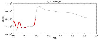
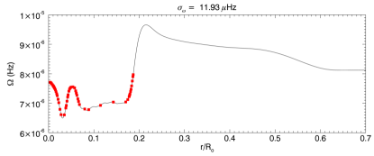
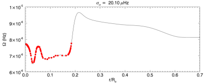
Figure 6: Position of the critical layers for retrograde IGWs for three different frequencies, superimposed with the rotational velocity profile in the star.

First of all, we only take into account retrograde waves because the prograde ones are damped immediately after their excitation (see § 4.4.2). Moreover, in the left panel of Fig. 7, we have represented in logarithmic scale the luminosity of a given IGW at the moment of its initial stochastic excitation by the turbulent convection as a function of its degrees $l$ and $m$, following the spectrum adopted in Talon & Charbonnel (2005). The difference between the three plots is the value of the excitation frequency $\sigma_{w}$. Thanks to this representation, we can see that the maximum of excitation lies in a domain where $l$ and $m$ are close and quite small. Moreover, it shows that for each excitation frequency, the amplitude of the excited wave depends on $l$ and $m$, and may be close to zero. As a consequence, some critical layers represented in Fig. 6 may belong to a non-excited wave, or to a wave completely damped at this depth. Fortunately, obtained results show that some waves really meet their critical layer.

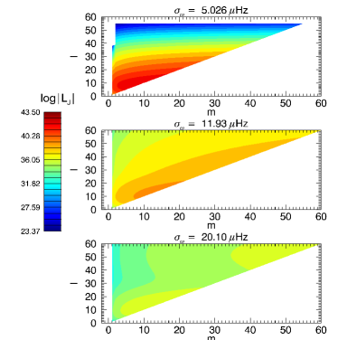
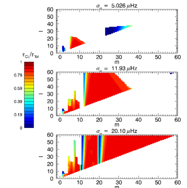
Figure 7: Left: Luminosity of the waves at the location of their excitation as function of $l$ and $m$. Right: Ratio between $\tau_{CL}$ and $\tau_{tot}=\tau_{CL}+\tau_{\mathrm{rad}}$ (see Eq. (6.2.3)).

6.2.2 Interaction between waves and critical layers

Concerning the way these latters interact with the surrounding fluid, the theory predicts two possible regimes depending on the value of the Richardson number $\mathrm{Ri}_{c}$ at the critical level. In our simulation, it appears that for every detected critical layer, the relation $\mathrm{Ri}_{c}>\frac{1}{4}\frac{m^{2}}{l\left(l+1\right)}$, which correponds to the stable regime, is verified. As a consequence, we establish that the second unstable regime (with the associated possible tunneling or over-reflection and transmission) does not occur for the solar-like star of our simulation; forthcoming studies may explore other types of stars at different evolutionary stages, to see if this regime can occur. Therefore, for the solar-type star studied here, we only implement in STAREVOL the terms related to stable critical layers: each time a wave passes through a critical layer, it is thus damped with a coefficient $e^{-\pi\sqrt{\frac{l(l+1)}{m^{2}}\mathrm{Ri}_{c}-\frac{1}{4}}}$ (see Eq. 88).

6.2.3 Effect of critical layers

Since all interactions between waves and critical layers are of the same kind in the studied star, we can concentrate on the quantitative importance of their effect on the transport of angular momentum. We know that in the stable regime (§5.2.2.), the wave passing through its critical layer is damped by the factor given in Eq. 88) that is added to radiative damping (here $P_{\rm r}\!<\!\!<\!1$ and the viscous damping is thus negligible), which has already been taken into account in previous works (e.g. Talon & Charbonnel, 2005). In the right panel of Figure 7, we thus choose to represent the ratio between $\tau_{\rm CL}$, the rate of attenuation due to the passage of the wave through its stable critical layer and the sum $\tau_{\rm tot}$ of this rate and the one of the radiative damping. The explicite formula is

$$\frac{\tau_{\rm CL}}{\tau_{\rm tot}}=$$

$$\frac{2\pi\sqrt{\frac{l(l+1)}{m^{2}}\mathrm{Ri}_{c}-\frac{1}{4}}}{2\pi\sqrt{\frac{l(l+1)}{m^{2}}\mathrm{Ri}_{c}-\frac{1}{4}}\!+\!\left[l\left(l+1\right)\right]^{\frac{3}{2}}\displaystyle\int_{r_{c}}^{r_{\mathrm{zc}}}{\kappa\frac{NN_{T}^{2}}{\sigma^{4}}\left(\frac{N^{2}}{N^{2}-\sigma^{2}}\right)^{\frac{1}{2}}\frac{1}{r^{3}}\mathrm{d}r}}\hbox{.}$$

On the contrary of the left panel, here are represented only waves which meet a critical layer. That is the reason why several white zones are seen. They correspond to the waves which have been attenuated before reaching the depth of their critical layer. In the case of low $\sigma_{w}$ (upper panels in Fig. 7), the high degree waves ($l>45$) are simply not excited, as we can see on the right. In red zones, the role of critical layers is important in comparison with the radiative damping while dark blue regions are those where the radiative damping dominates . Therefore, this figure shows that critical layers should be taken into account.

6.2.4 Evolution of the rotation profile

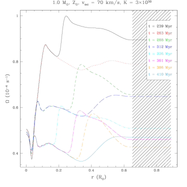
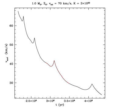
Figure 8: Evolution of the rotation profile where the role of the critical layers in the transport of angular momentum is taken into account. The curves are labelled according to the corresponding ages in Gyr. Parameters are indicated above where K is the braking constant. Right : Comparison between the evolution of the rotation with (red) and without (black) taking into account the effect of the critical layers.

Let us now concentrate on the evolution of the rotation profile when momentum deposition due to the interaction between waves and critical layers is taken into account. The other transport mechanism (IGWs’ radiative damping effects, the shear-induced turbulence and the meridional circulation) have been previously implemented in the code (Talon & Charbonnel, 2005).

In the center of the star, the rotation velocity is lower and increases the radiative damping of retrograde waves (see Eq. 72). This forms an angular momentum extraction front which propagates from the core to the surface to damp the differential rotation. Three fronts are seen in the top panel of Fig. 8 and have the same form that those already obtained in Talon & Charbonnel (2005). To isolate the action of critical layers on the evolution of the rotation profile, we have superimposed in the bottom panel of Fig. 8 the surface velocity as function of the evolution time with (black line) and without (red line) critical layer effects between $2.8\times 10^{8}$ and $3.5\times 10^{8}$ years. Both curves are nearly identical wich shows that despite their local action showed in Fig. 6, IGWs’ stable critical layers do not disturb the dynamical evolution of surface velocity in the case of the studied star. This can be easily understood since the radiative damping becomes mostly efficient around critical layers’ positions because of its dependance on $\sigma^{-4}$. Moreover, if in Talon & Charbonnel (2005), the IGWs action and the shear-induced turbulence have been added as uncoupled physical mechanisms, it has been demonstrated that in the upper region ($r>r_{c}$) where IGWs are propagative, the coefficient $\nu_{V}$ is negligible, while in the inner one ($r<r_{c}$) the differential rotation has been damped, leading to the same result with a transport dominated by the meridional circulation.

This clearly indicates that unstable critical layers will lead to major modification of the transport of angular momentum in stellar interiors. A systematic exploration of different type of stars for different evolutionary stages will be undertaken in a near future to explore their possible existence. Moreover, in order to give quantitative informations, it is necessary to improve the way waves are excited in this model. A future work will implement a prescription about penetrative convection processes. The best way to do it is to use a realistic numerical simulation of such mechanism to obtain the excitation spectrum at the base of the convective zone (Rogers & Glatzmaier, 2005; Brun et al., 2011; Alvan et al., 2012).

7 Conclusion

In this paper, we study in details a new mechanism of interaction between IGWs and the shear of the mean flow that occurs at co-rotation layers in stably stratified stellar radiation zones. Taking advantage of the work realized in the literature about atmospheric and oceanic fluids, we highlight the similarities with such stellar regions and propose an analytical approach adapted to the related case of deep spherical shells. Then, the use of spherical coordinates brings differences in the equations and make their resolution more complicated but the final results are comparable. We then demonstrate the intrinsic couplings between IGWs and the shear-induced instabilities and turbulence that can thus not be added linearly as done previously in stellar evolution literature. Then, we highlight the existence of two regimes where the interactions between IGWs and the shear at critical layers are strongly different:

• in the first case, the fluid is stable and IGWs amplitude is overdamped by the critical layer compared to the classical case where only radiative and viscous dampings are taken into account;

• in the second case, the fluid is unstable and turbulent and the critical layer acts as a secondary excitation region. Indeed, through over-reflection/transmission (when $|R|>1$ and $|T|>1$) energy is taken from the unstable shear that increase the amplitude of an incident IGW. Moreover, even in the case of simple reflection and transmission where $|R|<1$ and $|T|<1$, this demonstrate the existence of IGWs ”tunneling” through unstable regions as identified by Sutherland & Yewchuk (2004) in laboratory experiments and by Brown & Sutherland (2007); Nault & Sutherland (2007) in Geophysics.

Therefore, these mechanisms opens a new field of investigations concerning angular momentum tranport processes by IGWs in stellar interiors.

Indeed, even if according to our first evolutionary calculations with STAREVOL, only the first stable regime exists in solar-type stars, we expect to find stars where the unstable regime and possible tunneling or over-reflection/transmission take place. Moreover, while the formalism presented in this work is general, several uncertainties remain. First, concerning the stochastic excitation of IGWs by convection, the model used in our evolutionnary code certainly underestimates the wave flux since it considers only the volumetric excitation in the bulk of the convective envelope while convective penetration should be also taken into account. This will influence the measured action of critical layers since it is proportional to the initial IGWs amplitude. Then, only retrograde waves are simulated here, considering that prograde ones are immediately damped and do not penetrate deeply in the radiation zone. This should normaly not affect our results because the critical layers we detected are located in the deep radiation zone, but formal equations take both types of waves into account.

The last point to bear in mind is that no latitudinal dependence for the angular velocity is considered here. We explained the reason of this choice in the introduction but one must not forget this approximation. Finally, since our goal is to get a complete and coherent picture of the transport of angular momentum in stellar radiation zones for every stellar type or evolutionary stage, it will be important to extend this work to the cases of gravito-inertial waves, where the action of Coriolis and centrifugal accelerations is considered (e.g. Lee & Saio, 1997; Dintrans & Rieutord, 2000; Mathis, 2009; Ballot et al., 2010) and of magneto-gravito-inertial waves, when radiation zones are magnetized (e.g. Rudraiah & Venkatachalappa, 1972; Kim & MacGregor, 2003; MacGregor & Rogers, 2011; Mathis & de Brye, 2012).

Appendix A: Validity of the JWKB approximation

The form of the equation to solve is:

$$\frac{\mathrm{d}^{2}\Psi}{\mathrm{d}r^{2}}=f\left(r\right)\Psi\left(r\right)\hbox{.}$$ (93)

The first step is to introduce the Liouville transformation (e.g. Olver, 1974), i.e.:

$$W\left(r\right)=f^{1/4}\Psi\hbox{, and }\xi\left(r\right)=\int^{r}f^{1/2}{\rm d}r^{\prime}\hbox{.}$$ (94)

We deduce :

$$\frac{\mathrm{d}W}{\mathrm{d}\xi} = \frac{1}{4}f^{-5/4}f^{\prime}\Psi+f^{-1/4}\Psi^{\prime}\hbox{,}$$ (95)

$$\frac{\mathrm{d}^{2}W}{\mathrm{d}\xi^{2}} = -\frac{5}{16}f^{-11/4}f^{\prime 2}\Psi+\frac{1}{4}f^{-7/4}f^{\prime\prime}\Psi+f^{-3/4}\Psi^{\prime\prime}\hbox{,}$$ (96)

and Eq. (93) becomes

$$\frac{\mathrm{d}^{2}W}{\mathrm{d}\xi^{2}}=\left[1+\Phi\left(r\right)\right]W\hbox{,}$$ (97)

where $\Phi=\displaystyle\frac{4ff^{\prime\prime}-5f^{\prime 2}}{16f^{3}}$.
In the present case we have $f\left(r\right)=-k_{V}^{2}\left(r\right)=-\displaystyle\frac{l(l+1)}{r^{2}}\left(\displaystyle\frac{N^{2}}{\sigma^{2}}-1\right)$. The WKBJ approximation is available when $N^{2}\gg\sigma^{2}$. Consequently, we get

$$f\approx-l(l+1)\frac{1}{r^{2}}\frac{N^{2}}{\sigma^{2}}\hbox{,}$$ (98)

$$f^{\prime}\left(r\right)\approx l(l+1)\frac{2N^{2}}{r^{2}\sigma^{3}}m\bar{\Omega}^{\prime}\hbox{,}$$ (99)

$$f^{\prime\prime}\left(r\right)\approx-l(l+1)6m^{2}\frac{N^{2}\bar{\Omega}^{\prime 2}}{r^{2}\sigma^{4}}\hbox{,}$$ (100)

and

$$\Phi(r)\approx-\frac{1}{4}\frac{m^{2}}{l(l+1)}\frac{\left(\frac{\mathrm{d}\bar{\Omega}}{\mathrm{d}r}\right)^{2}r^{2}}{N^{2}}\equiv-\frac{1}{4}\frac{m^{2}}{l(l+1)}{\mathrm{R}_{i}}\hbox{,}\\$$ (101)

where $\mathrm{Ri}$ is the Richardson number of the fluid defined in Eq.(3).

At last, we obtain that the condition for applying the WKBJ approximation is $|\Phi|\ll 1$ which leads to $\mathrm{Ri}\gg\displaystyle\frac{1}{4}\frac{l(l+1)}{m^{2}}$.

Appendix B: Mathematical treatment for the non-perfect fluid case

Let us introduce

$$\chi_{l,m} = \int_{a}^{b}{e^{\eta t}v\left(t\right)dt}\hbox{,}$$ (102)

where $a$ and $b$ are the limits of a domain which will be defined later. The equation of propagation can then be written

$$\frac{1}{P_{\mathrm{r}}}t^{6}v+\left(1+\frac{1}{P_{\mathrm{r}}}\right)\frac{\mathrm{d}}{\mathrm{d}t}\left(t^{4}v\right)+\frac{\mathrm{d}^{2}}{\mathrm{d}t^{2}}\left(t^{2}v\right)+\mathrm{Ri}_{c}v=0\hbox{,}$$ (103)

and

$$\left[-\left(1+\frac{1}{P_{\mathrm{r}}}\right)t^{4}ve^{\eta t}-\frac{\mathrm{d}}{\mathrm{d}t}\left(t^{2}v\right)e^{\eta t}+zt^{2}ve^{\eta t}\right]_{a}^{b}=0\hbox{.}$$ (104)

The new variable $u$ defined by $v=t^{-2}e^{-\frac{1}{3}t^{3}}u$ transforms the original equation into

$$\frac{\mathrm{d}^{2}u}{\mathrm{d}t^{2}}-\left(1-\frac{1}{P_{\mathrm{r}}}\right)t^{2}\frac{\mathrm{d}u}{\mathrm{d}t}+\frac{l(l+1)}{m^{2}}\mathrm{Ri}_{c}\frac{1}{t^{2}}u=0\hbox{.}$$ (105)

Then, we introduce $s=Dt^{3}$ where $D\in\mathbb{C}^{*}$:

$$9s^{2}\frac{\mathrm{d}^{2}u}{\mathrm{d}s^{2}}+\left[6s-\frac{3s^{2}}{D}\left(1-\frac{1}{P_{\mathrm{r}}}\right)\right]\frac{\mathrm{d}u}{\mathrm{d}s}+\frac{l(l+1)}{m^{2}}\mathrm{Ri}_{c}u=0\hbox{.}$$ (106)

Finally, $u=s^{-1/3}Ve^{\frac{1}{6D}\left(1-\frac{1}{P_{\mathrm{r}}}\right)s}$ leads to:

$$9s^{2}\frac{\mathrm{d}^{2}V}{\mathrm{d}s^{2}}+ \left[2+\frac{l(l+1)}{m^{2}}\mathrm{Ri}_{c}+\frac{s}{D}\left(1-\frac{1}{P_{\mathrm{r}}}\right)\right.$$ (108)

$$-\left.\frac{s^{2}}{4D^{2}}\left(1-\frac{1}{P_{\mathrm{r}}}\right)^{2}\right]V=0$$

To obtain the final equation, we define:

$$D=-\frac{1}{3}(1-\frac{1}{P_{\mathrm{r}}})\hbox{,}$$ (109)

$$M_{l,m}^{2}=\frac{1}{4}-\frac{2+\frac{l(l+1)}{m^{2}}\mathrm{Ri}_{c}}{9}\hbox{,}$$ (110)

$$\Lambda=-\frac{1}{3}\hbox{.}$$ (111)

and we get the following Whittaker equation:

$$\frac{\mathrm{d}^{2}V}{\mathrm{d}s^{2}}+\left(\frac{\frac{1}{4}-M_{l,m}^{2}}{s^{2}}+\frac{\Lambda}{s}-\frac{1}{4}\right)V=0\hbox{.}$$ (113)

References

- Abramowitz & Stegun (1965) Abramowitz, M. & Stegun, I. 1965, Handbook of mathematical functions, ed. D. Publication
- Aerts et al. (2010) Aerts, C., Christensen-Dalsgaard, J., & Kurtz, D. W. 2010, Asteroseismology
- Alvan et al. (2012) Alvan, L., Brun, A. S., & Mathis, S. 2012, in SF2A-2012: Proceedings of the Annual meeting of the French Society of Astronomy and Astrophysics. Eds.: S. Boissier, 289–293
- Asplund et al. (2005) Asplund, M., Grevesse, N., & Sauval, A. J. 2005, in Astronomical Society of the Pacific Conference Series, Vol. 336, Cosmic Abundances as Records of Stellar Evolution and Nucleosynthesis, ed. T. G. Barnes III & F. N. Bash, 25
- Baldwin & Roberts (1970) Baldwin, P. & Roberts, P. H. 1970, Mathematika
- Ballot et al. (2010) Ballot, J., Lignières, F., Reese, D. R., & Rieutord, M. 2010, A&A, 518, A30
- Barker (2011) Barker, A. J. 2011, MNRAS, 414, 1365
- Barker & Ogilvie (2010) Barker, A. J. & Ogilvie, G. I. 2010, MNRAS, 404, 1849
- Beck et al. (2012) Beck, P. G., Montalban, J., Kallinger, T., et al. 2012, Nature, 481, 55
- Belkacem et al. (2009) Belkacem, K., Samadi, R., Goupil, M. J., et al. 2009, A&A, 494, 191
- Booker & Bretherton (1967) Booker, J. & Bretherton, F. 1967, J. Fluid Mech., 27, 513
- Braithwaite & Spruit (2004) Braithwaite, J. & Spruit, H. C. 2004, Nature, 431, 819
- Brown & Sutherland (2007) Brown, G. L. & Sutherland, B. R. 2007, Atmosphere-Ocean, 45, 47
- Brun et al. (2011) Brun, A. S., Miesch, M. S., & Toomre, J. 2011, ApJ, 742, 79
- Brun & Zahn (2006) Brun, A. S. & Zahn, J.-P. 2006, A&A, 457, 665
- Chapman & Lindzen (1970) Chapman, S. & Lindzen, R. 1970, Atmospheric tides. Thermal and gravitational
- Cowling (1941) Cowling, T. G. 1941, MNRAS, 101, 367
- Cunha et al. (2006) Cunha, K., Hubeny, I., & Lanz, T. 2006, ApJ, 647, L143
- Decressin et al. (2009) Decressin, T., Mathis, S., Palacios, A., et al. 2009, A&A, 495, 271
- Deheuvels et al. (2012) Deheuvels, S., Garcia, R., Chaplin, W. J., et al. 2012, The astrophysical journal, 756, 19
- Dintrans et al. (2005) Dintrans, B., Brandenburg, A., Nordlund, Å., & Stein, R. F. 2005, A&A, 438, 365
- Dintrans & Rieutord (2000) Dintrans, B. & Rieutord, M. 2000, A&A, 354, 86
- Drazin & Reid (2004) Drazin, P. G. & Reid, W. H. 2004, Hydrodynamic Stability
- Duez & Mathis (2010) Duez, V. & Mathis, S. 2010, A&A, 517, A58
- Eckart (1961) Eckart, C. 1961, Physics of Fluids, 4, 791
- Ferguson et al. (2005) Ferguson, J. W., Alexander, D. R., Allard, F., et al. 2005, ApJ, 623, 585
- Gaige (1993) Gaige, Y. 1993, A&A, 269, 267
- Garaud & Garaud (2008) Garaud, P. & Garaud, J. D. 2008, Monthly Notices of the Royal Astronomical Society, 391, 1239
- Garcia et al. (2007) Garcia, R. A., Turck-Chièze, S., Jiménez-Reyes, S. J., et al. 2007, Science, 316, 1591
- Garcia Lopez & Spruit (1991) Garcia Lopez, R. J. & Spruit, H. C. 1991, ApJ, 377, 268
- Goldreich & Kumar (1990) Goldreich, P. & Kumar, P. 1990, Astrophysical Journal, 363, 694
- Goldreich et al. (1994) Goldreich, P., Murray, N., & Kumar, P. 1994, Astrophysical Journal, 424, 466
- Goldreich & Nicholson (1989) Goldreich, P. & Nicholson, P. D. 1989, ApJ, 342, 1079
- Gough & McIntyre (1998) Gough, D. & McIntyre, M. 1998, Nature, 394, 755
- Hazel (1967) Hazel, P. 1967, J. Fluid Mech., 30, 775
- Iglesias & Rogers (1996) Iglesias, C. A. & Rogers, F. J. 1996, ApJ, 464, 943
- Kim & MacGregor (2003) Kim, E.-j. & MacGregor, K. B. 2003, ApJ, 588, 645
- Kippenhahn & Weigert (1990) Kippenhahn, R. & Weigert, A. 1990, S&T, 80, 504
- Knobloch & Spruit (1982) Knobloch, E. & Spruit, H. C. 1982, A&A, 113, 261
- Koppel (1964) Koppel, D. 1964, JMP, 5
- Lagarde et al. (2012) Lagarde, N., Decressin, T., Charbonnel, C., et al. 2012, A&A, 543, A108
- Lecoanet & Quataert (2012) Lecoanet, D. & Quataert, E. 2012, ArXiv e-prints
- Lee & Saio (1997) Lee, U. & Saio, H. 1997, ApJ, 491, 839
- Lighthill (1986) Lighthill, J. 1986, Provided by the SAO/NASA Astrophysics Data System
- Lindzen & Barker (1985) Lindzen, R. & Barker, A. 1985, J. Fluid Mech., 151, 189
- MacGregor & Rogers (2011) MacGregor, K. B. & Rogers, T. M. 2011, Sol. Phys., 270, 417
- Maeder (2003) Maeder, A. 2003, A&A, 399, 263
- Maeder (2009) Maeder, A. 2009, Physics, Formation and Evolution of Rotating Stars
- Maeder & Meynet (2001) Maeder, A. & Meynet, G. 2001, A&A, 373, 555
- Mathis (2009) Mathis, S. 2009, A&A, 506, 811
- Mathis (2010) Mathis, S. 2010, Astronomische Nachrichten, 331, 883
- Mathis & de Brye (2012) Mathis, S. & de Brye, N. 2012, A&A, 540, A37
- Mathis et al. (2004) Mathis, S., Palacios, A., & Zahn, J.-P. 2004, A&A, 425, 243
- Mathis & Zahn (2004) Mathis, S. & Zahn, J.-P. 2004, A&A, 425, 229
- Mathis & Zahn (2005) Mathis, S. & Zahn, J.-P. 2005, A&A, 440, 653
- Nault & Sutherland (2007) Nault, J. T. & Sutherland, B. R. 2007, Physics of Fluids, 19, 016601
- Ogilvie & Lin (2007) Ogilvie, G. I. & Lin, D. N. C. 2007, ApJ, 661, 1180
- Olver (1974) Olver. 1974, Asymptotics and Special Functions, ed. A. Press
- Prat & Lignières (2013) Prat, V. & Lignières, F. 2013, ArXiv e-prints
- Press (1981) Press, W. 1981, ApJ, 245, 286
- Reimers (1975) Reimers, D. 1975, Circumstellar envelopes and mass loss of red giant stars (Problems in stellar atmospheres and envelopes.), 229–256
- Rieutord (1986) Rieutord, M. 1986, Geophysical and Astrophysical Fluid Dynamics, 39, 163
- Ringot (1998) Ringot, O. 1998, PhD thesis, Ecole doctorale d’astronomie d’Ile de France
- Rogers & Glatzmaier (2005) Rogers, T. M. & Glatzmaier, G. A. 2005, MNRAS, 364, 1135
- Rogers et al. (2012) Rogers, T. M., Lin, D. N. C., & Lau, H. H. B. 2012, ApJ, 758, L6
- Rudraiah & Venkatachalappa (1972) Rudraiah, N. & Venkatachalappa, M. 1972, Journal of Fluid Mechanics, 52, 193
- Schatzman (1993) Schatzman, E. 1993, Astronomy and Astrophysics (ISSN 0004-6361), 279, 431
- Strugarek et al. (2011) Strugarek, A., Brun, A. S., & Zahn, J.-P. 2011, A&A, 532, A34
- Sutherland & Yewchuk (2004) Sutherland, B. R. & Yewchuk, K. 2004, Journal of Fluid Mechanics, 511, 125
- Talon & Charbonnel (2005) Talon, S. & Charbonnel, C. 2005, A&A, 440, 981
- Talon & Charbonnel (2008) Talon, S. & Charbonnel, C. 2008, A&A, 482, 597
- Talon & Zahn (1997) Talon, S. & Zahn, J.-P. 1997, Astronomy and Astrophysics, 317, 749
- Teschl (2011) Teschl, G. 2011, Ordinary Differential Equations and Dynamical Systems (American Mathematical Society, Providence, Rhode Island)
- Turck-Chièze & Couvidat (2011) Turck-Chièze, S. & Couvidat, S. 2011, Reports on Progress in Physics, 74, 086901
- Van Duin & Kelder (1986) Van Duin, C. & Kelder, H. 1986, J. Fluid. Mech., 169, 293
- Zahn (1992) Zahn, J. 1992, A&A
- Zahn (1975) Zahn, J.-P. 1975, A&A, 41, 329
- Zahn et al. (1997) Zahn, J.-P., Talon, S., & Matias, J. 1997, A&A, 322, 320