Moment LMI approach
to LTV impulsive control

Abstract

In the 1960s, a moment approach to linear time varying (LTV) minimal norm impulsive optimal control was developed, as an alternative to direct approaches (based on discretization of the equations of motion and linear programming) or indirect approaches (based on Pontryagin’s maximum principle). This paper revisits these classical results in the light of recent advances in convex optimization, in particular the use of measures jointly with hierarchy of linear matrix inequality (LMI) relaxations. Linearity of the dynamics allows us to integrate system trajectories and to come up with a simplified LMI hierarchy where the only unknowns are moments of a vector of control measures of time. In particular, occupation measures of state and control variables do not appear in this formulation. This is in stark contrast with LMI relaxations arising usually in polynomial optimal control, where size grows quickly as a function of the relaxation order. Jointly with the use of Chebyshev polynomials (as a numerically more stable polynomial basis), this allows LMI relaxations of high order (up to a few hundreds) to be solved numerically.

1 Introduction

In the 1960s, it was realized that many physically relevant problems of optimal control were inappropriately formulated in the sense that the optimum control law (a function of time and/or state) cannot be found if the admissible functional space is too small. This observation was the main driving force of the papers [17, 18, 20] which introduce optimal control problems formulated in the space of measures. The approach is well summarized in the textbook [15], which contains some (academic) examples of optimal control problems without solutions. This motivated the introduction of many concepts of functional analysis (density, completeness, duality, separability) in control engineering, building up on the advances on mathematical control theory and calculus of variations. As promoted in [15], an optimal control problem should be formulated in the dual of a Banach space which is large enough for the solution to be attained.

Most of the literature on numerical optimal control focuses on direct approaches (based on discretization of the equations of motions and linear programming) or indirect approaches (based on the necessary optimal conditions of Pontryagin’s maximum principle). When applied to optimal control problems whose optima cannot be attained, these numerical approaches typically face difficulties. In this context, we believe that it is timely to revisit classical results by Neustadt [17] on the formulation of optimal control problems for linear time varying (LTV) systems as a problem of moments, where the decision variables (from which an optimal control law can be extracted) are measures subject to a finite number of linear constraints.

There is an important literature, especially from the 1960s, on moment formulations to optimal control of ordinary differential equations (ODEs) and partial differential equations (PDEs), see e.g. [3] and references therein, as well as the comments of [7, p. 586]. Currently, this approach is not frequently used by engineers, and in our opinion this may be due, on the one hand, to the technicality of the underlying concepts of functional analysis, and, on the other hand, to the absence of numerical methods to deal satisfactorily with optimization problems in large functional spaces such as spaces of measures or distributions. Regarding the first point, we strongly recommend the textbook [15] which is a very readable account of elementary functional analysis useful for engineers. Regarding the second point, there has been recent advances in convex optimization, especially semidefinite programming (optimization over linear matrix inequalities, LMIs), for solving numerically generalized problems of moments, i.e. linear programming (LP) problems in Banach spaces of measures, see [12, 8] and references therein.

Our contribution is therefore to revisit the classical formulation by Neustadt [17] in the light of recent advances on LMI hierarchies for solving generalized problems of moments. In our previous work [11], we formulated polynomial optimal control problems with semialgebraic state and control constraints as generalized problems of moments that can be solved with asymptotically converging LMI hierarchies. The optimal control problem is relaxed to an LP problem in the space of occupation measures, which are measures of time, state and control encoding the trajectories of the system. The main drawback of this approach is the rapid growth of the size of the LMI problems in the hierarchy, making the approach applicable to small-size problems only (say at most 3 states and 2 controls). In the current paper, which focuses on the specific case of LTV dynamics depending affinely on the control variable, we first replace control variables by interpreting them as measures of time. This is similar to our previous work [6] which also dealt with impulsive control design in a more general setting. Second, we get rid of the state variables by integrating numerically the LTV ODE. This is possible because the ODE depends linearly on the state and the control. As a result, the optimal control problem is relaxed to an LP on measures depending only on time. It follows that there is no need for an LMI hierarchy since in the univariate case finite-dimensional moment LMI conditions are necessary and sufficient. However, there is still a hierarchy of LMI conditions in connection with the polynomial approximations of increasing degree we use to model the integrated system trajectories. To deal with those high degree univariate polynomials and moment matrices, we use Chebyshev polynomials instead of monomials. Indeed, high degree Chebyshev polynomials behave much better numerically than monomials, and we can rely on functionalities of the chebfun package for Matlab [22, 23] to integrate the LTV ODE and manipulate polynomials. To illustrate the above methodology, we show on some examples how to obtain very good approximations of impulse times and amplitudes of an optimal solution.

2 Relaxed linear optimal control

Consider the linear time varying (LTV) optimal control problem

$$\begin{array}[]{rcll}q^{*}&:=&\inf&\displaystyle\|u\|_{1}:=\sum_{j=1}^{m}\int_{t_{I}}^{t_{F}}|u_{j}(t)|dt\\ &&\mathrm{s.t.}&\dot{x}(t)=A(t)x(t)+B(t)u(t)\\ &&&x(t_{I})\in{\mathbb{R}}^{n}\quad\mathrm{given}\\ &&&x(t_{F})\in{\mathbb{R}}^{n}\quad\mathrm{given}\end{array}$$ (1)

where the minimization is w.r.t. a vector of control functions $u_{j}\in L^{1}([t_{I},t_{F}])$, $j=1,\ldots,m$, and $A\in L^{\infty}([t_{I},t_{F}];{\mathbb{R}}^{n\times n})$, $B\in C([t_{I},t_{F}];{\mathbb{R}}^{n\times m})$, on a given bounded time interval $[t_{I},t_{F}]\subset{\mathbb{R}}$.

In general the infimum is not attained, and the optimal control problem is relaxed to

$$\begin{array}[]{rcll}p^{*}&:=&\inf&\displaystyle\|\mu\|_{TV}:=\sum_{j=1}^{m}\int_{t_{I}}^{t_{F}}|\mu_{j}|(dt)\\ &&\mathrm{s.t.}&x(dt)=A(t)x(t)dt+B(t)\mu(dt)\\ &&&x(t_{I})\in{\mathbb{R}}^{n}\quad\mathrm{given}\\ &&&x(t_{F})\in{\mathbb{R}}^{n}\quad\mathrm{given}\end{array}$$ (2)

where the minimization is w.r.t. a vector of (signed) measures $\mu_{j}\in M([t_{I},t_{F}])$, $j=1,\ldots,m$, and $\|\mu\|_{TV}$ denotes the total variation, or norm, of vector measure $\mu$. A measure in $M([t_{I},t_{F}])$ of finite norm is identified (by a representation theorem of F. Riesz, see e.g. [19, Section 21.5]) as a continuous linear functional acting on the space of continuous functions $C([t_{I},t_{F}])$.

Problem (2) is a relaxation of problem (1) since we enlarge the space of admissible controls. Indeed, problem (1) is equivalent to problem (2) restricted to measures which are absolutely continuous w.r.t. time, i.e. $\mu_{j}(dt)=u_{j}(t)dt$ for some $u_{j}\in L^{1}([t_{I},t_{F}])$, $j=1,\ldots,m$. The motivation for introducing relaxed problem (2) is as follows.

Lemma 1

The infimum is attained in problem (2) and it is equal to the infimum of problem (1), i.e. $q^{*}=p^{*}$.

The proof of Lemma 1 is relegated to the end of Section 3. We will introduce a numerical method to deal directly with relaxed problem (2) in measure space $M$, bypassing the potential difficulties coming from the fact that the infimum in problem (1) is typically not attained in function space $L^{1}$. Before this, we need to reformulate optimal control problem (2) as a problem of moments.

3 Problem of moments

Now we integrate the differential equation in problem (2) to obtain an equivalent problem of moments. For more details, see e.g. [5, Section 2.2].

Let $f_{i}\in W^{1,1}([t_{I},t_{F}];{\mathbb{R}}^{n})$ denote the absolutely continuous solution of the Cauchy problem $\dot{f_{i}}(t)=A(t)f_{i}(t)$ with $f_{i}(t_{I})$ equal to the $i$-th column of $I_{n}$, the $n$-by-$n$ identity matrix, for $i=1,\ldots,n$. The matrix

$$F(t):=\left[\begin{array}[]{ccc}f_{1}(t)&\cdots&f_{n}(t)\end{array}\right]\in W^{1,1}([t_{I},t_{F}];{\mathbb{R}}^{n\times n})$$

therefore satisfies the matrix ODE

$$\dot{F}(t)=A(t)F(t),\quad F(t_{I})=I_{n},\quad t\in[t_{I},t_{F}].$$

From [5, Theorem 2.2.3], matrix $F^{-1}(t)$ is differentiable and any function $x(t)$ satisfying

$$x(t_{F})=F(t_{F})\left[x(t_{I})+\int_{t_{I}}^{t_{F}}F^{-1}(t)B(t)\mu(dt)\right]$$

is a solution to the differential equation

$$x(dt)=A(t)x(t)dt+B(t)\mu(dt),\quad t\in[t_{I},t_{F}].$$ (3)

Letting

$$\begin{array}[]{rcl}G(t)&:=&(F^{-1}(t)B(t))^{T}\\ &=&\left[\begin{array}[]{ccc}g_{1}(t)&\cdots&g_{n}(t)\end{array}\right]\in C([t_{I},t_{F}];{\mathbb{R}}^{m\times n}),\\[10.00002pt] h&:=&F^{-1}(t_{F})x(t_{F})-x(t_{I})\in{\mathbb{R}}^{m},\end{array}$$

we can replace the differential equation (3) with the integral equation:

$$\int_{t_{I}}^{t_{F}}G^{T}(t)\mu(dt)=h.$$

It follows that problem (2) can be written equivalently as

$$\begin{array}[]{rcll}p^{*}&=&\min&\displaystyle\|\mu\|_{TV}\\ &&\mathrm{s.t.}&\displaystyle\langle g_{i},\mu\rangle=h_{i},\quad i=1,\ldots,n\end{array}$$ (4)

where

$$\langle g_{i},\mu\rangle:=\int_{t_{I}}^{t_{F}}g^{T}_{i}(t)\mu(dt)=\sum_{j=1}^{m}\int_{t_{I}}^{t_{F}}g_{i,j}(t)\mu_{j}(dt)$$

denotes the duality bracket between $C([t_{I},t_{F}];{\mathbb{R}}^{m})$ and its dual $M([t_{I},t_{F}];{\mathbb{R}}^{m})$, a bilinear form pairing $C([t_{I},t_{F}];{\mathbb{R}}^{m})$ and $M([t_{I},t_{F}];{\mathbb{R}}^{m})$. Problem (4) is a problem of moments consisting of finding $m$ measures subject to $n$ linear constraints.

Proof: (of Lemma 1) The proof that the infimum of problem (2) is attained follows from [17, Theorem 1]. Moreover, in [17, Theorem 4] it is shown that there exists a solution $\mu$ to problem (4), hence to problem (2), which is the (signed) sum of at most $n$ Dirac measures. Finally, it is shown in [17, pp. 45-46] that there is a sequence of functions $u^{k}\in L^{1}([t_{I},t_{F}];{\mathbb{R}}^{m})$, $k=1,2,\ldots$ which are admissible for problem (1), i.e. $\mu(dt)=u^{k}(t)dt$ satisfies the constraints in problem (4), and which are such that $\lim_{k\to\infty}\|u^{k}\|_{1}=p^{*}$. $\Box$

4 Primal and dual conic LP

By decomposing each signed measure $\mu_{j}$ as a difference of two nonnegative measures (using the Jordan decomposition theorem, see e.g. [19, Section 17.2]), i.e.

$$\mu_{j}=\mu^{+}_{j}-\mu^{-}_{j},\quad\mu^{+}_{j}\geq 0,\quad\mu^{-}_{j}\geq 0,\quad j=1,\ldots,m,$$

problem (4) can be written as a linear programming (LP) problem on the cone of nonnegative measures

$$\begin{array}[]{rcll}p^{*}&=&\inf&\displaystyle\langle 1,\mu^{+}\rangle+\langle 1,\mu^{-}\rangle\\ &&\mathrm{s.t.}&\displaystyle\langle g_{i},\mu^{+}\rangle-\langle g_{i},\mu^{-}\rangle=h_{i},\quad i=1,\ldots,n\\ &&&\mu^{+}\geq 0,\quad\mu^{-}\geq 0\end{array}$$ (5)

where $1$ denotes the $m$-dimensional vector of functions identically equal to one, and the above minimization is w.r.t. two vector-valued nonnegative measures $\mu^{+}\in M([t_{I},t_{F}];{\mathbb{R}}^{m})$, $\mu^{-}\in M([t_{I},t_{F}];{\mathbb{R}}^{m})$. It is easy to show that problem (5) is equivalent to problem (4).

Problem (5) is the dual of the following LP on the cone of nonnegative continuous functions (see [21] for details of the derivation):

$$\begin{array}[]{rcll}d^{*}&=&\sup&\displaystyle\sum_{i=1}^{n}y_{i}h_{i}\\ &&\mathrm{s.t.}&\displaystyle z^{+}(t):=1+\sum_{i=1}^{n}y_{i}g_{i}(t)\geq 0\quad t\in[t_{I},t_{F}]\\ &&&z^{-}(t):=\displaystyle 1-\sum_{i=1}^{n}y_{i}g_{i}(t)\geq 0\quad t\in[t_{I},t_{F}]\end{array}$$ (6)

where the maximization is w.r.t. a vector $y\in{\mathbb{R}}^{n}$ parametrizing two vector-valued nonnegative continuous functions $z^{+}\in C([t_{I},t_{F}];{\mathbb{R}}^{m})$, $z^{-}\in C([t_{I},t_{F}];{\mathbb{R}}^{m})$. Denoting

$$\|z\|_{\infty}:=\sup_{t\in[t_{I},t_{F}],j=1,\ldots,m}|z_{j}(t)|$$

for any $z\in C([t_{I},t_{F}];{\mathbb{R}}^{m})$, remark that LP problem (6) can be also written as

$$\begin{array}[]{rcll}d^{*}&=&\sup&h^{T}y\\ &&\mathrm{s.t.}&\|G(t)y\|_{\infty}\leq 1.\end{array}$$ (7)

Lemma 2

There is no duality gap between LP (5) and (6), i.e. $p^{*}=d^{*}$.

Proof: Define the vector $r(\mu^{+},\mu^{-})\in{\mathbb{R}}^{n+1}$ with entries $r_{0}(\mu^{+},\mu^{-}):=\langle 1,\mu^{+}\rangle+\langle 1,\mu^{-}\rangle$, $r_{i}(\mu^{+},\mu^{-}):=\langle g_{i},\mu^{+}\rangle-\langle g_{i},\mu^{-}\rangle$, $i=1,\ldots,n$ and the set $R:=\{r(\mu^{+},\mu^{-})\>:\>(\mu^{+},\mu^{-})\in M^{2m}_{+}\}\subset{\mathbb{R}}^{n+1}$ where $M^{2m}_{+}$ denotes the cone of nonnegative measures in $M([t_{I},t_{F}];{\mathbb{R}}^{2m})$. Let us invoke [1, Theorem 3.10] which states that $p^{*}=d^{*}$ provided $p^{*}$ is finite and $R$ is closed. Finiteness of $p^{*}$ follows immediately since we minimize the total variation. To prove closedness, we have to show that all accumulation points of any sequence $r(\mu^{+}_{n},\mu^{-}_{n})$ belong to $R$. Since the supports of the measures are compact and $p^{*}$ is finite, hence $\mu^{+}$ and $\mu^{-}$ are bounded, the sequence $(\mu^{+}_{n},\mu^{-}_{n})$ is bounded. By the weak-* compactness of the unit ball in the Banach space of bounded signed measures with compact support (Alaoglu’s Theorem, see e.g. [15, Section 5.10] or [19, Section 15.1]), there is a subsequence $(\mu^{+}_{n_{k}},\mu^{-}_{n_{k}})$ that converges weakly-* to an element $(\mu^{+},\mu^{-})\in M^{2m}_{+}$. As $1$ and all $g_{i}$ belong to $C([t_{I},t_{F}];{\mathbb{R}}^{m})$ then $\lim_{k\to\infty}r(\mu^{+}_{n_{k}},\mu^{-}_{n_{k}})=r(\mu^{+},\mu^{-})\in R$. $\Box$

Zero duality gap implies that any optimal pair $((\mu^{+},\mu^{-}),(z^{+},z^{-}))$ solving LPs (5-6) satisfies the complementarity conditions

$$\langle z^{+}_{j},\mu^{+}_{j}\rangle=0,\quad\langle z^{+}_{j},\mu^{-}_{j}\rangle=0,\quad j=1,\ldots,m.$$

This means that the support of each measure $\mu^{+}_{j}$, resp. $\mu^{-}_{j}$, is included in the set $\{t\in[t_{I},t_{F}]:z^{+}_{j}(t)=0\}$, resp. $\{t\in[t_{I},t_{F}]:z^{-}_{j}(t)=0\}$, for $j=1,\ldots,m$.

Note that formulation (7) of the dual problem dates back to the work of Neustadt [17] and was preferred to the primal formulation for numerical solution of the optimal control problem. One objective of this paper is to show that the recent advances on the moment problem give an efficient computation procedure for the primal problem. In particular, one obtains very good approximations of an optimal solution of (5) (impulse times and amplitudes).

Remark 1

The vector $G(t)y$ involved in LP problem (6) is known as the primer vector introduced in the seminal work [13]. This primer vector is defined as the velocity adjoint vector arising by the application of Pontryagin’s maximum principle to optimal trajectory problems. The primer vector must satisfy Lawden’s well-known necessary conditions for an optimal impulsive trajectory.

5 Integration of the LTV ODE

In order to compute matrix $F(t)$, the last step before obtaining a tractable problem, we have to integrate numerically the ODE $\dot{x}(t)=A(t)x(t)$. Matrix $G(t)$ solves numerically the LTV system of equations $F(t)G^{T}(t)=B(t)$. In practice, we use the Matlab software package Chebfun [22] to build Chebyshev polynomial interpolants of the problem data $A(t)$ and $B(t)$. Some of its specialized numerical routines to compute $F(t)$ and $G(t)$ have been used here.

We want to characterize the error of approximating $G(t)$ by its Chebyshev polynomial interpolant on $d$ points, see [23] for an introduction on this subject. Define $G_{d}(t)$ as the Chebyshev interpolant of $G(t)$ on $d$ points. Assume furthermore that the error induced by algebraic manipulations for obtaining $G_{d}(t)$ can be properly controlled. Then the approximation error $e_{d}:=\|G_{d}-G\|_{\infty}$ for large $d$ is conditionned by the regularity of $G(t)$. We recall the main results of approximation theory which can all be found in [23]:

• if $G(t)$ is $k$-times continuously differentiable, then $e_{d}\rightarrow 0$ at the algebraic rate of $\mathcal{O}(d^{-k})$ as $d\rightarrow\infty$;

• if $G(t)$ is $k$-times differentiable with its $k$-th derivative of bounded variation, then the algebraic rate is $\mathcal{O}(d^{-k})$;

• if $G(t)$ is analytic, then there exists a positive $\rho$ such that the algebraic rate is $\mathcal{O}(\rho^{-d})$.

This imposes some minimal requirements for $A(t)$ and $B(t)$ for our numerical approach to work. Indeed, assuming $A(t)$ of bounded variation and $B(t)$ differentiable with derivative of bounded variation guarantees that the error converges to zero for large approximation orders.

We now show that if $e_{d}\rightarrow 0$ as $d\rightarrow\infty$, we can build a hierarchy of moment relaxations of (4) involving only approximate data and converging to $p^{*}$. For this, let $F_{d}(t)$ denote the Chebyshev interpolant of $F(t)$ on $d$ points, and let $h_{d}:=F^{-1}_{d}(t_{F})x(t_{F})-F^{-1}_{d}(t_{I})x(t_{I})$.

Lemma 3

Consider the following relaxed moment problem with approximate data:

$$\begin{array}[]{rcl}\tilde{p}_{d}^{*}=&\min&\|\mu\|_{TV}\\ &\mathrm{s.t.}&\left|\int\!G_{d}^{T}\,d\mu-h_{d}\right|\leq e_{d}\,(\|B\|\,|x(t_{F})|+\|\mu\|_{TV}).\end{array}$$ (8)

Then $\tilde{p}_{d}^{*}\uparrow p^{*}$ as $d\rightarrow\infty$

Proof: By the same argument as Lemma 1, a solution for (8) is attained. Furthermore, any solution $\mu^{*}$ of (4) is feasible for (8), as

$$\begin{array}[]{rcl}\left|\int\!G_{d}^{T}\,d\mu^{*}-h_{d}\right|&\leq&\left|\int\!G^{T}\,d\mu^{*}-h\right|+\left|\int\!(G_{d}^{T}-G^{T})\,d\mu^{*}\right|+||B||\,|x(t_{F})|\,\left|h_{d}-h\right|\\ &\leq&0+e_{d}\,||\mu^{*}||_{\textrm{TV}}+e_{d}\,||B||\,|x(t_{F})|.\end{array}$$

Therefore, $\tilde{p}_{e}^{*}\leq p^{*}$ holds.

For the convergence, consider the auxiliary relaxed problem with the true data instead:

$$\begin{array}[]{rcl}p_{d}^{*}=&\min&\|\mu\|_{TV}\\ &\mathrm{s.t.}&\left|\int\!G^{T}\,d\mu-h\right|\leq 2e_{d}\,(\|B\|\,|x(t_{F})|+\|\mu\|_{TV}).\end{array}$$ (9)

By similar arguments, we have that $p_{d}^{*}\leq\tilde{p}_{d}^{*}\leq p^{*}$. Because of this uniform bound on the minimizers of (9), standard arguments (see for instance the second part of the Banach-Saks-Steinhaus theorem in [19, Section 13.5]) show that $p^{*}\leq\liminf p_{d}^{*}$, which show indeed that $p_{d}^{*}\rightarrow p^{*}$, hence $\tilde{p}_{d}^{*}\rightarrow p^{*}$. $\Box$

6 Solving the LP on measures

To summarize, we have formulated our LTV optimal control problem as a primal-dual LP pair (5-6). The coefficients in these LP problems are entries of matrix function $G(t)$ and vector $h$. These data are calculated by numerical integration, using Chebyshev polynomial approximations, as explained in the last section. For a given degree $d$ of the polynomial approximation, LP problem (5) is a particular instance of a generalized problem of moments. It can be seen as an extension of the approach of [11] which was originally designed for classical optimal control problems with polynomial dynamics. Alternatively, it can also be understood as an application of the approach of [6], but after integration of the ODE, which is here possible because of linearity of the dynamics in the state and control.

An infinite-dimensional LP on measures can be solved approximately by a hierarchy of finite-dimensional linear matrix inequality (LMI) problems, see [11, 6, 9] for details (not reproduced here). The main idea behind the hierarchy is to manipulate each measure via its moments truncated to degree $d$. Note that here the measures are univariate (depending on time only). Therefore, for a problem involving polynomials up to degree $d$, the $d$-th LMI condition is necessary and sufficient. The hierarchy presented in this paper comes thus from the polynomial approximation of the continuous data, not from the moment truncation. In contrast, when dealing with multivariate measures as in [11, 6, 9], we use a hierarchy of necessary LMI conditions which become sufficient only asymptotically.

Generally speaking, the number of variables in an LMI relaxation of order $d$ of a multivariate measure LP grows polynomially in $d$, but the exponent is the number of variables entering the measures. If the number of variables is equal to 5 or more, the growth is fast, and only LMI relaxation of small orders can be solved at a reasonable computational cost. It is therefore crucial to reduce as much as possible the number of variables entering the measures, so as to reduce the overall computational burden. One contribution of our paper is precisely to show that for LTV optimal control problems, we can manipulate measures of the time variable only. This allows for LMI relaxations of large order to be solved, with $d$ a few hundreds.

7 Examples

7.1 Scalar polynomial example

Consider the optimal control problem (1):

$$\begin{array}[]{rcll}p^{*}&=&\inf&\displaystyle\|u\|_{1}:=\int_{0}^{1}|u(t)|dt\\ &&\mathrm{s.t.}&\dot{x}(t)=t(1-t)u(t)\\ &&&x(0)=0,\quad x(1)=1\end{array}$$

where the minimization is w.r.t. a function $u\in L^{1}([0,1])$. Since $L^{1}([0,1])$ is not the dual of any normed space, the problem must be relaxed to the optimal control problem (2):

$$\begin{array}[]{rcll}p^{*}&=&\min&\displaystyle\|\mu\|_{TV}:=\int_{0}^{1}|\mu|(dt)\\ &&\mathrm{s.t.}&x(dt)=t(1-t)\mu(dt)\\ &&&x(0)=0,\quad x(1)=1\end{array}$$

where the minimization is now w.r.t. a measure $\mu\in M([0,1])$. Following the approach of Section 3, we readily obtain $F(t)=1$, $G(t)=t(1-t)$ and hence the moment problem (4):

$$\begin{array}[]{rcll}p^{*}&=&\min&\|\mu\|_{TV}\\ &&\mathrm{s.t.}&\displaystyle\langle t(1-t),\mu\rangle:=\int_{0}^{1}t(1-t)\mu(dt)=1.\end{array}$$

Decomposing $\mu=\mu^{+}-\mu^{-}$ as a difference of two nonnegative measures we obtain the LP (5):

$$\begin{array}[]{rcll}p^{*}&=&\inf&\langle 1,\mu^{+}\rangle+\langle 1,\mu^{-}\rangle\\ &&\mathrm{s.t.}&\displaystyle\langle t(1-t),\mu^{+}\rangle-\langle t(1-t),\mu^{-}\rangle=1\\ &&&\mu^{+}\geq 0,\quad\mu^{-}\geq 0\end{array}$$

where the minimization is w.r.t. measures $\mu^{+},\mu^{-}$, and the LP (6):

$$\begin{array}[]{rcll}d^{*}&=&\sup&y\\ &&\mathrm{s.t.}&-1\leq t(1-t)y\leq 1,\quad\forall~{}t\in[0,1]\end{array}$$

where the maximization is w.r.t. $y\in{\mathbb{R}}$. For this latter problem, we readily obtain that the maximum $d^{*}=4$ is attained for the choice $y=4$. Since polynomial $4t(1-t)$ attains its maximum at $t=\frac{1}{2}$ it follows from the discussion after Lemma 2 that the optimal measure solution is $\mu^{+}=4\delta_{\frac{1}{2}}$ and $\mu^{-}=0$, achieving $p^{*}=4$.

As this problem has polynomial data, we can readily find the optimal solution, with the following GloptiPoly 3 script [8], instead of using the approximation techniques of Section V:

>> mpol tp tn;
>> mp = meas(tp); % measure \mu^+
>> mn = meas(tn); % measure \mu^-
>> P = msdp(min(mass(mp)+mass(mn)), ...
   mom(tp*(1-tp))-mom(tn*(1-tn)) == 1, ...
   tp*(1-tp) >= 0 ... % support of \mu^+
   tn*(1-tn) >= 0);   % support of \mu^-
>> [stat, obj] = msol(P);
obj =
    4.0000
>> double(mmat(mp)) % moment mat. of \mu^+
ans =
    4.0000    2.0001
    2.0001    1.0001
>> double(mmat(mn)) % moment mat. of \mu^-
ans =
   1.0e-08 *
    0.2673    0.2036
    0.2036    0.2186

7.2 Nonsmooth trajectories

This example is meant to illustrate the numerical difficulty we may face when integrating LTV ODEs with discontinuous state matrix $A(t)$. Consider the following optimal control problem (1):

$$\begin{array}[]{rcll}p^{*}&=&\inf&\|u\|_{1}\\ &&\mathrm{s.t.}&\dot{x}(t)=\mathrm{sign}(t)x(t)+u(t)\\ &&&x(-1)=-1,\quad x(1)=1\end{array}$$

where the minimization is w.r.t. a function $u\in L^{1}([-1,1])$. Upon solving the ODE $\dot{F}(t)=\mathrm{sign}(t)F(t)$, $F(-1)=1$ we obtain $F(t)=e^{-1+|t|}$, $G(t)=e^{1-|t|}$ and hence the moment problem (4):

$$\begin{array}[]{rcll}p^{*}&=&\inf&\|\mu\|_{TV}\\ &&\mathrm{s.t.}&\langle e^{1-|t|},\mu\rangle=2\end{array}$$

where the minimization is now w.r.t. a signed measure $\mu\in M([-1,1])$. The dual problem (6) reads:

$$\begin{array}[]{rcll}d^{*}&=&\sup&2y\\ &&\mathrm{s.t.}&-1\leq ye^{1-|t|}\leq 1\quad\forall~{}t\in[-1,1]\\ \end{array}$$

where the maximization is w.r.t. a real scalar $y$. The optimal dual solution can easily be found analytically as $y^{*}=e^{-1}$, from which it follows that the optimal primal solution is $\mu^{*}=2e^{-1}\delta_{t=0}$.

$d$	$\|G-G_{d}\|_{\infty}$	$|p^{*}-p_{d}|/|p^{*}|$
10	0.1995	0.1243
20	0.0899	0.0555
30	0.0579	0.0357
40	0.0427	0.0263
50	0.0338	0.0208
60	0.0280	0.0172
70	0.0239	0.0147
80	0.0208	0.0128
90	0.0184	0.0114
100	0.0166	0.0102

Table 1: Approximation errors vs. polynomial approximation orders for discontinuous dynamics.

If we want to apply the numerical integration approach of Section 5, discontinuity of $A(t)=\mathrm{sign}(t)$ turns out to be a problem. Indeed, we can check that $G(t)$ presents a cusp at $t=0$. That is, for an even number $d$ of Chebyshev interpolation points, the maximum interpolation error $\|G-G_{d}\|_{\infty}$ is located where the optimal impulse should be, while for an odd $d$ the interpolant is exact at the cusp. In Table 1 we present the approximation errors on function $G$ and on the optimal cost $p_{d}^{*}$ as functions of $d$, found by our numerical method. The results exhibit the expected linear decrease in the approximation error, resulting in a linear decrease in the optimal cost. The error for moderate orders $(d\approx 100)$ is acceptable though far from excellent.

$d$	$\|G-G_{d}\|_{\infty}$	$|p^{*}-p_{d}|/|p^{*}|$
2	$2.1187\cdot 10^{-1}$	$3.4307\cdot 10^{-3}$
4	$1.0851\cdot 10^{-3}$	$1.0406\cdot 10^{-5}$
6	$2.2540\cdot 10^{-6}$	$1.5281\cdot 10^{-8}$
8	$2.5115\cdot 10^{-9}$	$1.3166\cdot 10^{-11}$
10	$1.7422\cdot 10^{-12}$	$5.9438\cdot 10^{-13}$
12	$1.1336\cdot 10^{-15}$	$5.8093\cdot 10^{-12}$
14	$<10^{-15}$	$1.3729\cdot 10^{-11}$
16	$<10^{-15}$	$3.1846\cdot 10^{-12}$
18	$<10^{-15}$	$2.5462\cdot 10^{-10}$

Table 2: Approximation errors vs. polynomial approximation orders for piecewise analytic dynamics.

Now, if we split the time interval around the cusp, the restrictions of $G(t)$ on the intervals $[-1,0]$ and $[0,1]$ are respectively $G_{L}(t):=e^{1+t}$ and $G_{R}(t):=e^{1-t}$ which are both analytic. The updated moment problem with piecewise analytic data reads:

$$\begin{array}[]{rcll}p^{*}&=&\inf&\|\mu_{L}\|_{TV}+\|\mu_{R}\|_{TV}\\ &&\mathrm{s.t.}&\displaystyle\int_{-1}^{0}G_{L}(t)\mu_{L}(dt)+\int_{0}^{1}G_{R}(t)\mu_{R}(dt)=2.\end{array}$$

In Table 2, we present the updated polynomial approximation errors, which show the expected exponential decrease. For the cost, the decrease is exponential until a relative error of about $10^{-10}$ after which the error comes from the semidefinite solver (used to solve the LMI hierarchy of the moment problem), not from the polynomial approximation.

7.3 A fuel-optimal linear impulsive guidance rendezvous problem for an elliptic reference orbit

$$\begin{array}[]{@{}r@{\:}c@{\:}l@{}}A(t)\>&=\hfil\>&\left[\begin{array}[]{cccc}0&0&1&0\\ 0&0&0&1\\ \bar{n}^{2}e\,\cos\nu(t)\left(\dfrac{1+e\,\cos\nu(t)}{1-e^{2}}\right)^{3}&-2\,\bar{n}^{2}\,e\,\sin\nu(t)\left(\dfrac{1+e\,\cos\nu(t)}{1-e^{2}}\right)^{3}&0&2\bar{n}\dfrac{\left(1+e\,\cos\nu(t)\right)^{2}}{\left(1-e^{2}\right)^{3/2}}\\ 2\,\bar{n}^{2}\,e\,\sin\nu(t)\left(\dfrac{1+e\,\cos\nu(t)}{1-e^{2}}\right)^{3}&\bar{n}^{2}(3+e\cos\nu(t))\left(\dfrac{1+e\cos\nu(t)}{1-e^{2}}\right)^{3}&-2\bar{n}\dfrac{\left(1+e\,\cos\nu(t)\right)^{2}}{\left(1-e^{2}\right)^{3/2}}&0\end{array}\right]\\ B(t)\>&=\hfil\>&\left[\begin{array}[]{cc}0&0\\ 0&0\\ \bar{n}^{2}&0\\ 0&\bar{n}^{2}\end{array}\right]\end{array}$$ (10)

Finally, an illustration based on a realistic case of a far range rendezvous in a linearized gravitational field is given. The general framework of the minimum-fuel fixed-time coplanar rendezvous problem in a linear setting is recalled in [2], where an indirect method based on primer vector theory is proposed. Under Keplerian assumptions and for an elliptic reference orbit, the complete rendezvous problem may be decoupled between the out-of-plane rendezvous problem for which an analytical solution may be found and the coplanar problem. Therefore, only a coplanar elliptic rendezvous problem based on the Tschauner-Hempel equations [24] is studied thereafter. The associated optimal control problem (1) has a 4-dimensional ($n=4$) state vector composed of the relative positions (denoted here $x(t)$, $z(t)$) and respective velocities in the LVLH frame [14] and a 2-dimensional ($m=2$) control vector $u(t)$ (one control in the $x$-direction, one control in the $z$-direction). The state space matrices $A(t)$ and $B(t)$ are given in equ. (10), with $\bar{n}=34.0094$ is the mean angular motion, $e=4.0000\cdot~{}10^{-3}$ is the eccentricity, $\nu(t)$ is the true anomaly of the reference orbit satisfying for all $t\geq 0$ the Kepler equation:

$$\begin{array}[]{rcl}\bar{n}t&=&E(t)-e\,\sin E(t)\\ \tan\dfrac{\nu(t)}{2}&=&\left(\dfrac{1+e}{1-e}\right)^{1/2}\tan\dfrac{E(t)}{2}\end{array}$$

where $E(t)$ is the eccentric anomaly.

For this problem, $G(t)$ can be approximated below the $10^{-8}$ resolution of the SDP solver by polynomials of degree $100$ on the given time interval. This implies that the problem can be solved numerically by LMI relaxations of order $50$, with a computational load of a few seconds. The assembly of $G(t)$ using Chebfun routines take a few seconds as well. All of this was done without any sort of problem-specific optimization, and with standard Matlab code.

To solve the optimal control problem, direct methods based on the solution of a linear programming (LP) problem can be used as in [16, 14]. For an a priori fixed number of impulsive maneuvers at given times, an LP problem is formulated and solved numerically. Its solution is therefore suboptimal, depending strongly upon the number of impulsions. This makes it hard to evaluate how far the solution could be from the global optimum.

The particular instance, studied in this paper, is borrowed from the PRISMA test bed and GNC experiments from [4]. PRISMA programme is a cooperative effort between the Swedish National Space Board (SNSB), the French Centre National d’Etudes Spatiales (CNES), the German Deutsche Zentrum für Luft- und Raumfahrt (DLR) and the Danish Danmarks Tekniske Universitet (DTU) [10]. Launched on June 15, 2010 from Yasny (Russia), it was intended to test in-orbit new guidance schemes (particularly autonomous orbit control) for formation flying and rendezvous technologies. This mission includes the FFIORD experiment led by CNES, which features a rendezvous maneuver (formation acquisition). To save fuel and allow for in-flight testing throughout the FFIORD experiment, the rendezvous maneuver must last several orbits. Duration of the rendezvous is approximately 14.25 orbital periods, each of duration $5920s$, i.e. $t_{I}=0$ and $t_{F}=84360$ in problem (1).

	2-impulse	LP (20 i.)	LP (2000 i.)	LMI
$t_{0}$	0	0	0	0
$t_{1}$	-	$8880$	2321	2140
$t_{2}$	-	$75480$	2363	82350
$t_{3}$	84360	$84360$	82334	-
$u(t_{0})$	$\begin{array}[]{c}0.02\\ -0.1985\end{array}$	$\begin{array}[]{c}0.0006\\ 0\end{array}$	$\begin{array}[]{c}0.0174\\ 0\end{array}$	$\begin{array}[]{c}0.0172\\ 0\end{array}$
$u(t_{1})$	-	$\begin{array}[]{c}0.0014\\ 0\end{array}$	$\begin{array}[]{c}0.0193\\ 0\end{array}$	$\begin{array}[]{c}0.0011\\ 0\end{array}$
$u(t_{2})$	-	$\begin{array}[]{c}-0.0146\\ 0\end{array}$	$\begin{array}[]{c}-0.0003\\ 0\end{array}$	$\begin{array}[]{c}-0.019\\ 0\end{array}$
$u(t_{3})$	$\begin{array}[]{c}-0.0215\\ 0.218\end{array}$	$\begin{array}[]{c}-0.0207\\ 0\end{array}$	$\begin{array}[]{c}-0.019\\ 0\end{array}$	-
cost m/s	$0.4588$	$0.04072$	0.03736	0.03736

Table 3: Comparisons of results of moment LMI approach, two-impulse solution and direct LP solution for 200 and 2000 impulses for the PRISMA case study

The moment LMI approach is compared to the classical 2-impulse solution and to the direct approach with 20 and 2000 pre-assigned evenly distributed impulses. These results are presented in Table 3, where $t_{k}$ are the impulsion times and $u(t_{k})$ the impulsion directions, for $k=0,1,2,3$. It is interesting to note that the 2-impulse solution has a prohibitive cost when compared to the optimal solution found by the direct method and the moment LMI approach. This is mainly due to the extra thrusts in the $z$-direction that are not necessary to realize this particular rendezvous. Indeed, a remarkable feature of the optimal solution is that it exhibits a terminal coast, unlike the 2-impulse and direct 20-impulse solution. Note also that the 2-impulse solution leads to a very different trajectory in the orbital plane as shown by Figure 1. The optimal fuel-cost computed via the moment LMI approach is less than half the one obtained in [4] via a pseudo-closed loop technique ($0.086$ m/s).

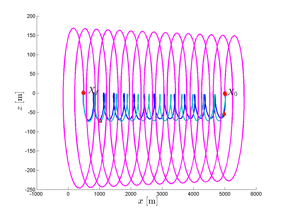
Figure 1: Trajectories in the orbital plane: 2-impulse solution (pink), optimal solution (blue), Direct 20-impulses solution (cyan).

Figure 2 shows the importance of the pre-assigned number of impulses for the direct method to recover the optimal solution. Indeed, for a small number of impulses, the solution given by the direct method is a crude approximation of the optimal solution obtained by the moment LMI approach and by the direct approach with 2000 pre-assigned impulses. The impulse locations are indicated on the trajectories (red triangles for the optimal solution and red squares for the 20-impulse solution). The differences of locations of the impulses for the four methods used on the PRISMA example are depicted on Figure 3.

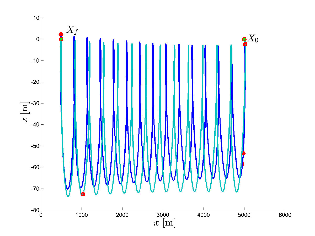
Figure 2: Trajectories in the orbital plane: optimal solution (blue), Direct 20-impulses solution (cyan) .

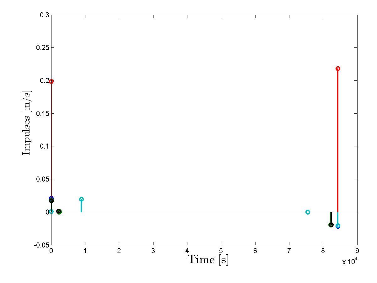
Figure 3: Impulses for 2-impulse solution (red and blue), direct 20-impulse solution (cyan), optimal solution (black).

8 Conclusion

In this paper, we revisit classic impulsive control theory from the 1960s with modern numerical tools stemming from convex programming and approximation theory. The theory leads to the reformulation of a control problem as a one-dimensional problem of moments. The numerical tools allow for its efficient numerical solution without any expert knowledge needed.

Several extensions of our work are possible and will be included in an extended version of this paper. First of all, the class of dynamics can easily be extended to cover those with a forced drift term, i.e. to dynamics

$$\dot{x}=A(t)x(t)+B(t)u(t)+w(t)$$

with $w(t)\in C^{1}([t_{I},t_{F}],\mathbb{R}^{n})$. The second main extension is to enforce positivity constraints on linear combinations of the states using additional positive measures. Finally, the method can also consider other norms of the form $||u(\cdot)||_{p}:=\int\!|u(t)|_{p}\,dt$ with $p=2,3,...$, instead of the $p=1$ case that is the focus of this paper. This can be done since norms with integer exponents are semidefinite representable.

For the specific case of orbital rendezvous as exemplified in Section 7.3, one can exploit the specific symmetries of (10) to approximate $G(t)$ off-line on half an orbital period, and partition the time interval accordingly such as presented in Ex. 7.2. This will lead to accurate, low order polynomial approximations, and one could expect to obtain computational loads compatible for an online implementation of a model predictive control loop.

References

- [1] E. J. Anderson, P. Nash. Linear programming in infinite-dimensional spaces: theory and applications. Wiley, New York, 1987.
- [2] D. Arzelier, M. Kara-Zaitri, C. Louembet, A. Delibasi. Using polynomial optimization to solve the fuel-optimal impulsive rendezvous problem. J. Guidance, Control and Dynamics, 34(5):1567-1572, 2011.
- [3] S. A. Avdonin, S. A. Ivanov. Families of exponentials: the method of moments in controllability problems for distributed parameter systems. Cambridge Univ. Press, UK, 1995.
- [4] J. C. Berges, S. Djalal, P. Y. Guidotti, M. Delpech. CNES formation flying experiment on PRISMA: spacecraft reconfiguration and rendezvous within FFIORD mission. Proc. Intl. ESA Conf. Guidance, Navigation and Control Systems, Karlovy Vary, Czech Republic, 2011.
- [5] A. Bressan, B. Piccoli. Introduction to the mathematical theory of control. Amer. Inst. Math. Sci., Springfield, MO, 2007.
- [6] M. Claeys, D. Arzelier, D. Henrion, J. B. Lasserre. Measures and LMI for impulsive optimal control with applications to space rendezvous problems. Proc. Amer. Control Conf., Montreal, Canada, 2012.
- [7] H. O. Fattorini. Infinite dimensional optimization and control theory. Cambridge Univ. Press, UK, 1999.
- [8] D. Henrion, J. B. Lasserre, J. Löfberg. GloptiPoly 3: moments, optimization and semidefinite programming. Optim. Meth. Softw. 24(4-5):761-779, 2009.
- [9] D. Henrion, M. Korda. Convex computation of the region of attraction of polynomial control systems. arXiv:1208.1751, Aug. 2012.
- [10] R. Larsson, S. Berge, P. Bodin, U. Jönsson. Fuel efficient relative orbit control strategies for formation flying and rendezvous within PRISMA. Proc. Annual AAS Rocky Mountain Guidance and Control Conference, AAS 06-025, pp. 25-40, Breckenridge, Colorado, 2006.
- [11] J. B. Lasserre, D. Henrion, C. Prieur, E. Trélat. Nonlinear optimal control via occupation measures and LMI relaxations. SIAM J. Control Opt. 47(4):1643-1666, 2008.
- [12] J. B. Lasserre. Moments, positive polynomials and their applications. Imperial College Press, London, UK, 2009.
- [13] D. F. Lawden. Optimal trajectories for space navigation. Butterworth, London, 1963.
- [14] C. Louembet, D. Arzelier, G. Deaconu, P. Blanc-Paques. Robust rendezvous planning under navigation and manoeuvering errors. Proc. Intl. ESA Conf. Guidance, Navigation and Control Systems, Karlovy Vary, Czech Republic, 2011.
- [15] D. G. Luenberger. Optimization by vector space methods. Wiley, New York, 1969.
- [16] J. B. Mueller, R. Larsson. Collision avoidance maneuver planning with robust optimization. Proc. Intl. ESA Conf. Guidance, Navigation and Control Systems, Tralee, County Kerry, Ireland, 2008.
- [17] L. W. Neustadt. Optimization, a moment problem and nonlinear programming. SIAM J. Control 2(1):33-53, 1964.
- [18] R. Rishel. An extended Pontryagin principle for control systems whose control laws contain measures. SIAM J. Control 3(2):191-205, 1965.
- [19] H. Royden, P. Fitzpatrick. Real analysis. 4th edition. Pearson Education, Boston, 2010.
- [20] W. W. Schmaedeke. Optimal control theory for nonlinear vector differential equations containing measures. SIAM J. Control 3(2):231-280, 1965.
- [21] A. Shapiro. On duality theory of conic linear programming. Chapter 7 in Semi infinite programming: Recent Advances. M. A. Goberna, M. A. López (Eds.), Kluwer Academic, Vol. 57, 2001.
- [22] L. N. Trefethen and others. Chebfun Version 4.2, The Chebfun Development Team, 2011. www.maths.ox.ac.uk/chebfun
- [23] L. N. Trefethen. Approximation theory and approximation practice. SIAM, Philadelphia, 2013.
- [24] J. Tschauner, P. Hempel. Rendevous zu einem in elliptischer Bahn umlaufenden Ziel. Astronautica Acta, II(2):104-109, 1965.