Joint Wireless Information and Energy Transfer in a Two-User MIMO Interference Channel

Abstract

This paper investigates joint wireless information and energy transfer in a two-user MIMO interference channel, in which each receiver either decodes the incoming information data (information decoding, ID) or harvests the RF energy (energy harvesting, EH) to operate with a potentially perpetual energy supply. In the two-user interference channel, we have four different scenarios according to the receiver mode – ($ID_{1}$, $ID_{2}$), ($EH_{1}$, $EH_{2}$), ($EH_{1}$, $ID_{2}$), and ($ID_{1}$, $EH_{2}$). While the maximum information bit rate is unknown and finding the optimal transmission strategy is still open for ($ID_{1}$, $ID_{2}$), we have derived the optimal transmission strategy achieving the maximum harvested energy for ($EH_{1}$, $EH_{2}$). For ($EH_{1}$, $ID_{2}$), and ($ID_{1}$, $EH_{2}$), we find a necessary condition of the optimal transmission strategy and, accordingly, identify the achievable rate-energy (R-E) tradeoff region for two transmission strategies that satisfy the necessary condition - maximum energy beamforming (MEB) and minimum leakage beamforming (MLB). Furthermore, a new transmission strategy satisfying the necessary condition - signal-to-leakage-and-energy ratio (SLER) maximization beamforming - is proposed and shown to exhibit a better R-E region than the MEB and the MLB strategies. Finally, we propose a mode scheduling method to switch between ($EH_{1}$, $ID_{2}$) and ($ID_{1}$, $EH_{2}$) based on the SLER.

I Introduction

Over the last decade, there has been a lot of interest to transfer energy wirelessly and recently, radio-frequency (RF) radiation has become a viable source for energy harvesting. It is nowadays possible to transfer the energy wirelessly with a reasonable efficiency over small distances and, furthermore, the wireless sensor network (WSN) in which the sensors are capable of harvesting RF energy to power their own transmissions has been introduced in industry ([1, 2, 3, 4] and references therein).

The energy harvesting function can be exploited in either transmit side [5, 6, 7, 8, 9] or receive side [10, 11, 12, 13]. For the energy harvesting transmitter, energy harvesting scheduling and transmit power allocation have been considered and, for the energy harvesting receiver, the management of information decoding and energy harvesting has been developed. Furthermore, because RF signals carry information as well as energy, “joint wireless information and energy transfer” in conjunction with the energy harvesting receiver has been investigated [10, 11, 12, 13]. That is, previous works have studied the fundamental performance limits and the optimal transmission strategies of the joint wireless information and energy transfer in the cellular downlink system with a single base station (BS) and multiple mobile stations (MSs) [12] and in the cooperative relay system [13] and in the broadcasting system [10, 11] with a single energy receiver and a single information receiver when they are separately located or co-located.

There have been very few studies of joint wireless information and energy transfer on the interference channel (IFC) models [14, 15, 16]. In [14, 15], the authors have considered a two-user single-input single-output (SISO) IFC and derived the optimal power scheduling at the energy harvesting transmitters that maximizes the sum-rate given harvested energy constraints. In [16], the authors have investigated joint information and energy transfer in multi-cell cellular networks with single-antenna BSs and single-antenna MSs. To the best of the authors’ knowledge, the general setup of multiple-input multiple-output (MIMO) IFC models accounting for joint wireless information and energy transfer has not been addressed so far.

As an initial step, in this paper, we investigate a joint wireless information and energy transfer in a two-user MIMO IFC, where each receiver either decodes the incoming information data (information decoding, ID) or harvests the RF energy (energy harvesting, EH) to operate with a potentially perpetual energy supply. Because practical circuits and hardware that harvest energy from the received RF signal are not yet able to decode the information carried through the same RF signal [10, 11, 17], we assume that the receiver cannot decode the information and simultaneously harvest energy. It is also assumed that the two (Tx 1,Tx 2) transmitters have knowledge of their local CSI only, i.e. the CSI corresponding to the links between a transmitter and all receivers (Rx 1, Rx 2). In addition, the transmitters do not share the information data to be transmitted and their CSI and, furthermore, the interference is assumed not decodable at the receiver nodes as in [18]. That is, Tx 1 (Tx 2) cannot transfer the information to Rx 2 (Rx 1). In a two-user IFC, we then have four different scenarios according to the Rx mode – ($ID_{1}$, $ID_{2}$), ($EH_{1}$, $EH_{2}$), ($EH_{1}$, $ID_{2}$), and ($ID_{1}$, $EH_{2}$). Because, for ($ID_{1}$, $ID_{2}$), the maximum information bit rate is unknown and finding the optimal transmission strategy is still an open problem in general, we investigate the achievable rate when a well-known iterative water-filling algorithm [19, 20, 21] is adopted for ($ID_{1}$, $ID_{2}$) with no CSI sharing between two transmitters. For ($EH_{1}$, $EH_{2}$), we derive the optimal transmission strategy achieving the maximum harvested energy. Because the receivers operate in a single mode such as ($ID_{1}$, $ID_{2}$) and ($EH_{1}$, $EH_{2}$), when the information is transferred, no energy is harvested from RF signals and vice versa. For ($EH_{1}$, $ID_{2}$) and ($ID_{1}$, $EH_{2}$), the achievable energy-rate (R-E) trade-off region is not easily identified and the optimal transmission strategy is still unknown. However, in this paper, we find a necessary condition of the optimal transmission strategy, in which one of the transmitters should take a rank-one energy beamforming strategy with a proper power control. Accordingly, the achievable R-E tradeoff region is identified for two different rank-one beamforming strategies - maximum energy beamforming (MEB) and minimum leakage beamforming (MLB). Furthermore, we also propose a new transmission strategy that satisfies the necessary condition - signal-to-leakage-and-energy ratio (SLER) maximization beamforming. Note that the SLER maximizing approach is comparable to the signal-to-leakage-and-noise ratio (SLNR) maximization beamforming [22, 23] which has been developed for the multi-user MIMO data transmission, not considering the energy transfer. The simulation results demonstrate that the proposed SLER maximization strategy exhibits wider R-E region than the conventional transmission methods such as MLB, MEB, and SLNR beamforming. Finally, we propose a mode scheduling method to switch between ($EH_{1}$, $ID_{2}$) and ($ID_{1}$, $EH_{2}$) based on the SLER that further extends R-E tradeoff region.

The rest of this paper is organized as follows. In Section II, we introduce the system model for two-user MIMO IFC. In Section III, we discuss the transmission strategy for two receivers on a single mode, i.e. ($ID_{1}$, $ID_{2}$) and ($EH_{1}$, $EH_{2}$). In Section IV, we derive the necessary condition for the optimal transmission strategy and investigate the achievable rate-energy (R-E) region for ($EH_{1}$, $ID_{2}$) and ($ID_{1}$, $EH_{2}$) and, in Section V, propose the SLER maximization strategy. In Section VI and Section VII, we provide several discussion and simulation results, respectively, and in Section VIII we give our conclusions.

Throughout the paper, matrices and vectors are represented by bold capital letters and bold lower-case letters, respectively. The notations $({\bf A})^{H}$, $({\bf A})^{\dagger}$, $({\bf A})_{i}$, $[{\bf A}]_{i}$, $tr({\bf A})$, and $\det({\bf A})$ denote the conjugate transpose, pseudo-inverse, the $i$th row, the $i$th column, the trace, and the determinant of a matrix ${\bf A}$, respectively. The matrix norm $\|{\bf A}\|$ and $\|{\bf A}\|_{F}$ denote the 2-norm and Frobenius norm of a matrix ${\bf A}$, respectively, and the vector norm $\|{\bf a}\|$ denotes the 2-norm of a vector ${\bf a}$. In addition, $(a)^{+}\triangleq\max(a,0)$ and ${\bf A}\succeq 0$ means that a matrix ${\bf A}$ is positive semi-definite. Finally, ${\bf I}_{M}$ denotes the $M\times M$ identity matrix.

II System model

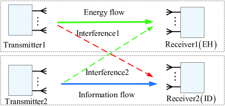
Figure 1: Two-user MIMO IFC in ($EH_{1}$, $ID_{2}$) mode.

We consider a two-user MIMO IFC system where two transmitters, each with $M_{t}$ antennas, are simultaneously transmitting their signals to two receivers, each with $M_{r}$ antennas, as shown in Fig. 1. Note that each receiver can either decode the information or harvest energy from the received signal, but it cannot execute the information decoding and energy harvesting at the same time due to the hardware limitations. That is, each receiver can switch between ID mode and EH mode at each frame or time slot. We assume that the transmitters have perfect knowledge of the CSI of their associated links (i.e. the links between a transmitter and all receivers) but do not share those CSI between them. In addition, $M_{t}=M_{r}=M$ for simplicity, but it can be extended to general antenna configurations. Assuming a frequency flat fading channel, which is static over several frames, the received signal ${\bf y}_{i}\in\mathbb{C}^{M\times 1}$ for $i=1,2$ can be written as

$${\bf y}_{1}={\bf H}_{11}{\bf x}_{1}+{\bf H}_{12}{\bf x}_{2}+{\bf n}_{1},$$

$${\bf y}_{2}={\bf H}_{21}{\bf x}_{1}+{\bf H}_{22}{\bf x}_{2}+{\bf n}_{2},$$ (1)

where ${\bf n}_{i}\in\mathbb{C}^{M\times 1}$ is a complex white Gaussian noise vector with a covariance matrix ${\bf I}_{M}$ and ${\bf H}_{ij}\in\mathbb{C}^{M\times M}$ is the normalized frequency-flat fading channel from the $j$th transmitter to the $i$th receiver such as $\sum_{l,k=1}^{M}|h_{ij}^{(l,k)}|^{2}=\alpha_{ij}M$ [24]. Here, $h_{ij}^{(l,k)}$ is the $(l,k)$th element of ${\bf H}_{ij}$ and $\alpha_{ij}\in[0,1]$. We assume that ${\bf H}_{ij}$ has a full rank. The vector ${\bf x}_{j}\in\mathbb{C}^{M\times 1}$ is the transmit signal, in which the independent messages can be conveyed, at the $j$th transmitter with a transmit power constraint for $j=1$ and $2$ as

$$E[\|{\bf x}_{j}\|^{2}]\leq P{\text{ for }}j=1\text{ and }2.$$ (2)

When the receiver operates in ID mode, the achievable rate at $i$th receiver, $R_{i}$, is given by [19]

$$R_{i}=\log\det({\bf I}_{M}+{\bf H}_{ii}^{H}{\bf R}_{-i}^{-1}{\bf H}_{ii}{\bf Q}_{i}),$$ (3)

where ${\bf R}_{-i}$ indicates the covariance matrix of noise and interference at the $i$th receiver, i.e.,

$${\bf R}_{-1}={\bf I}_{M}+{\bf H}_{12}{\bf Q}_{2}{\bf H}_{12}^{H},$$

$${\bf R}_{-2}={\bf I}_{M}+{\bf H}_{21}{\bf Q}_{1}{\bf H}_{21}^{H}.$$

Here, ${\bf Q}_{j}=E[{\bf x}_{j}{\bf x}_{j}^{H}]$ denotes the covariance matrix of the transmit signal at the $j$th transmitter and, from (2), $tr({\bf Q}_{j})\leq P$.

For EH mode, it can be assumed that the total harvested power $E_{i}$ at the $i$th receiver (more exactly, harvested energy normalized by the baseband symbol period) is given by

$$E_{i} = \zeta_{i}E[\|{\bf y}_{i}\|^{2}]$$ (4)

$$= \zeta_{i}tr\left(\sum_{j=1}^{2}{\bf H}_{ij}{\bf Q}_{j}{\bf H}_{ij}^{H}+{\bf I}_{M}\right),$$

where $\zeta_{i}$ denotes the efficiency constant for converting the harvested energy to electrical energy to be stored [3, 10]. For simplicity, it is assumed that $\zeta_{i}=1$ and the noise power is negligible compared to the transferred energy from each transmitters. That is,

$$E_{i} \approx tr\left(\sum_{j=1}^{2}{\bf H}_{ij}{\bf Q}_{j}{\bf H}_{ij}^{H}\right)$$ (5)

$$= tr\left({\bf H}_{i1}{\bf Q}_{1}{\bf H}_{i1}^{H}\right)+tr\left({\bf H}_{i2}{\bf Q}_{2}{\bf H}_{i2}^{H}\right)$$

$$= E_{i1}+E_{i2},$$

where $E_{ij}=tr\left({\bf H}_{ij}{\bf Q}_{j}{\bf H}_{ij}^{H}\right)$ denoting the energy transferred from the $j$th transmitter to the $i$th receiver.

Interestingly, when the receiver decodes the information data from the associated transmitter under the assumption that the signal from the other transmitter is not decodable [18], the signal from the other transmitter becomes an interference to be defeated. In contrast, when the receiver harvests the energy, it becomes a useful energy-transferring source. Fig. 1 illustrates an example of the receiving mode ($EH_{1}$, $ID_{2}$), where the interference1 (dashed red line) should be reduced for ID, while the interference2 (dashed green line) be maximized for EH. In what follows, for four possible receiving modes, we investigate the achievable rate-harvested energy tradeoff. In addition, the corresponding transmission strategy (more specifically, transmit signal design) is presented.

III Two receivers on a single mode

III-A Two IDs: maximum achievable sum rate

For the scenario ($ID_{1}$, $ID_{2}$), it is desirable to obtain the maximum achievable sum rate. That is, the problem can be formulated as follows:

$$(P1){\text{ maximize }} \sum_{i=1}^{2}R_{i}$$ (6)

subject to $$tr({\bf Q}_{j})\leq P,~{}{\bf Q}_{j}\succeq{\bf 0}\quad{\text{for }}j=1,2,$$ (7)

The solution of (P1) has been extensively considered in many previous communication researches [19, 20, 21], where the iterative water-filling algorithms have been developed to maximize the achievable rate in a distributed manner with no CSI sharing between the transmitters. This is briefly summarized in Algorithm 1:

Algorithm 1. Iterative Water-filling:

1. Initialize $n=0$ and ${\bf Q}_{j}^{(0)}\in\mathcal{Q}_{P}$ for $j=1,2$, where

   $$\mathcal{Q}_{P}\triangleq\{{\bf Q}\in\mathbb{C}^{M\times M}:{\bf Q}\succeq{\bf 0},tr({\bf Q})=P\}.$$ (8)

2. For $n=0:N_{max}$, where $N_{max}$ is the maximum number of iterations
        Update ${\bf Q}_{j}^{(n+1)}$ for $j=1,2$ as follows:

   $$\!{\bf Q}_{j}^{(n\!+\!1)}\!=\!\left\{\!\begin{array}[]{c}WF({\bf H}_{jj},{\bf R}_{-j}^{(n)},P),~{}\text{if ${\bf R}_{-j}^{(n)}$ is updated,\!}\!\\ {\bf Q}_{j}^{(n)},\quad\text{otherwise,}\end{array}\!\right.\!\!$$ (11)

   where ${\bf R}_{-j}^{(n)}$ indicates the covariance matrix of noise and interference in the $j$th receiver at the $n$th iteration, i.e.,

   $${\bf R}_{-1}^{(n)}={\bf I}_{M}+{\bf H}_{12}{\bf Q}_{2}^{(n)}{\bf H}_{12}^{H},$$

   $${\bf R}_{-2}^{(n)}={\bf I}_{M}+{\bf H}_{21}{\bf Q}_{1}^{(n)}{\bf H}_{21}^{H}.$$

   Note that ${\bf R}_{-j}^{(n)}$ is measured at each receiver similarly to the way it has been done in [19] and, furthermore, ${\bf Q}_{j}^{(n)}$ is computed at the receiver and reported to the transmitter through the zero-delay and error-free feedback link.

3. Finally, ${\bf Q}_{j}={\bf Q}_{j}^{N_{max}+1}$ for $j=1,2$.

Here, $WF()$ denotes the water-filling operator given as [19]:

$$WF({\bf H}_{ii},{\bf R},P)={\bf U}_{i}(\mu_{i}{\bf I}_{M}-{\bf D}_{i}^{-1})^{+}{\bf U}_{i}^{H},$$ (12)

where ${\bf U}_{i}$ and ${\bf D}_{i}$ are obtained from the eigenvalue decomposition of ${\bf H}_{ii}^{H}{\bf R}^{-1}{\bf H}_{ii}$. That is, ${\bf H}_{ii}^{H}{\bf R}^{-1}{\bf H}_{ii}={\bf U}_{i}{\bf D}_{i}{\bf U}_{i}^{H}$, and $\mu_{i}$ denotes the water level that satisfies the transmit power constraint as $tr\{(\mu_{i}{\bf I}_{M}-{\bf D}_{i}^{-1})^{+}\}=P$.

In the scenario ($ID_{1}$, $ID_{2}$), because both receivers decode the information, the harvested energy becomes zero.

III-B Two EHs: maximum harvested energy

For the scenario ($EH_{1}$, $EH_{2}$), both receivers want to achieve the maximum harvested energy. That is, the problem can be formulated as:

$$(P2){\text{ maximize }} \sum_{i=1}^{2}E_{i}$$ (13)

subject to $$tr({\bf Q}_{j})\leq P,~{}{\bf Q}_{j}\succeq{\bf 0}\quad{\text{for }}j=1,2,$$ (14)

The following proposition gives the optimal solution for the problem (P2).

Proposition 1

The optimal ${\bf Q}_{j}$ for (P2) has a rank equal to one and is given as ${\bf Q}_{j}=P[\bar{\bf V}_{j}]_{1}[\bar{\bf V}_{j}]_{1}^{H}$, where $\bar{\bf V}_{j}$ is a $M\times M$ unitary matrix obtained from the SVD of $\bar{\bf H}_{j}\triangleq\left[\begin{array}[]{c}{\bf H}_{1j}\\ {\bf H}_{2j}\end{array}\right]$. That is, $\bar{\bf H}_{j}=\bar{\bf U}_{j}\bar{\bf\Sigma}_{j}\bar{\bf V}_{j}^{H}$, where $\bar{\bf\Sigma}_{j}=diag\{\bar{\sigma}_{j,1},...,\bar{\sigma}_{j,M}\}$ with $\bar{\sigma}_{j,1}\geq...\geq\bar{\sigma}_{j,M}$.

Proof:

From (5),

$$\sum_{i=1}^{2}E_{i} = \sum_{i=1}^{2}tr\left(\sum_{j=1}^{2}{\bf H}_{ij}{\bf Q}_{j}{\bf H}_{ij}^{H}\right)$$ (15)

$$= \sum_{j=1}^{2}tr\left(\sum_{i=1}^{2}{\bf H}_{ij}{\bf Q}_{j}{\bf H}_{ij}^{H}\right)$$

$$= \sum_{j=1}^{2}tr\left(\bar{\bf H}_{j}{\bf Q}_{j}\bar{\bf H}_{j}^{H}\right)$$

Note that the covariance matrix ${\bf Q}_{j}$ can be written as ${\bf Q}_{j}={\bf V}_{j}{\bf D}_{j}^{2}{\bf V}_{j}^{H}$ where ${\bf V}_{j}$ is a $M\times M$ unitary matrix and ${\bf D}_{j}^{2}=diag\{d_{j,1}^{2},...,d_{j,M}^{2}\}$ with $\sum_{m=1}^{M}d_{j,m}^{2}\leq P$. Because $tr({\bf A}{\bf B})=tr({\bf B}{\bf A})$ for ${\bf A}\in\mathbb{C}^{m\times n}$ and ${\bf B}\in\mathbb{C}^{n\times m}$, (15) can be rewritten as

$$\sum_{i=1}^{2}E_{i}=\sum_{j=1}^{2}tr\left({\bf D}_{j}^{2}{\bf V}_{j}^{H}\bar{\bf H}_{j}^{H}\bar{\bf H}_{j}{\bf V}_{j}\right)=\sum_{j=1}^{2}\sum_{m=1}^{M}d_{j,m}^{2}\|\bar{\bf H}_{j}[{\bf V}_{j}]_{m}\|^{2}.$$ (16)

Because $\sum_{m=1}^{M}d_{j,m}^{2}\leq P$,

$$\sum_{m=1}^{M}d_{j,m}^{2}\|\bar{\bf H}_{j}[{\bf V}_{j}]_{m}\|^{2}\leq P\underset{m=1,...M}{\max}\|\bar{\bf H}_{j}[{\bf V}_{j}]_{m}\|^{2}.$$ (17)

Here, the equality holds when $d_{j,m^{\prime}}^{2}=P$ for $m^{\prime}=\arg\underset{m=1,...M}{\max}\|\bar{\bf H}_{j}[{\bf V}_{j}]_{m}\|^{2}$ and $d_{j,m}^{2}=0$ for $m\neq m^{\prime}$, which implies that ${\bf Q}_{j}$ has a rank equal to one and accordingly, it is given as ${\bf Q}_{j}=P[{\bf V}_{j}]_{m^{\prime}}[{\bf V}_{j}]_{m^{\prime}}^{H}$. Note that

$$\|\bar{\bf H}_{j}[{\bf V}_{j}]_{m^{\prime}}\|^{2}\leq\bar{\sigma}_{j,1}^{2},$$ (18)

where the equality holds when $[{\bf V}_{j}]_{m^{\prime}}=[\bar{\bf V}_{j}]_{1}$. Therefore, from (17) and (18), (16) is bounded as

$$\!\sum_{i=1}^{2}E_{i}\!=\!\sum_{j=1}^{2}\sum_{m=1}^{M}d_{j,m}^{2}\|\bar{\bf H}_{j}[\bar{\bf V}_{j}]_{m}\|^{2}\!\leq P(\bar{\sigma}_{1,1}^{2}+\bar{\sigma}_{2,1}^{2}),$$

and the equality holds when ${\bf Q}_{j}=P[\bar{\bf V}_{j}]_{1}[\bar{\bf V}_{j}]_{1}^{H}$. ∎

Note that each transmitter can design the transmit covariance matrix ${\bf Q}_{j}$ such that the transferred energy from each transmitter is maximized without considering other transmitter’s channel information and transmission strategy. That is, thanks to the energy conservation law, each transmitter transfers the energy through its links independently.

From Proposition 1, the transmit signal on each transmitter can be designed as ${\bf x}_{j}=\sqrt{P}[\bar{\bf V}_{j}]_{1}{\bf s}_{j}$, where ${\bf s}_{j}$ is any random signal with zero mean and unit variance. Because both receivers harvest the energy and are not able to decode the information, the achievable rate becomes zero.

IV One ID receiver and One EH receiver

In this section, without loss of generality, we will consider ($EH_{1}$, $ID_{2}$) - the first receiver harvests the energy and the second decodes information. The transmission strategy described below can also be applied to ($ID_{1}$, $EH_{2}$) without difficulty. Note that energy harvesting and information transfer occur simultaneously in the IFC, and accordingly, the achievable rate-energy region is not trivial compared to the scenarios ($EH_{1}$, $EH_{2}$) and ($ID_{1}$, $ID_{2}$).

IV-A A necessary condition for the optimal transmission strategy

Because information decoding is done only at the second receiver, by letting $R=R_{2}$ and $E=E_{1}=E_{11}+E_{12}$, we can define the achievable rate-energy region as:

$$\!C_{R\!-\!E}(P)\!\triangleq\!\Biggl{\{}\!(R,E):R\leq\log\det({\bf I}_{M}+{\bf H}_{22}^{H}{\bf R}_{-2}^{-1}{\bf H}_{22}{\bf Q}_{2}),\!$$

$$\!E\!\leq\!\sum_{\!j\!=\!1}^{\!2}tr({\bf H}_{1j}{\bf Q}_{j}{\bf H}_{1j}^{H}),tr({\bf Q}_{j})\!\leq\!P,{\bf Q}_{j}\!\succeq\!{\bf 0},j\!=\!1,\!2\!\Biggr{\}}\!.\!$$ (19)

Here, because EH and ID operations in the IFC interact with each other, the boundary of the rate-energy region is not easily characterized and is so far unknown. The following lemma gives a useful insight into the derivation of the optimal boundary.

Lemma 1

For ${\bf H}_{11}$ and ${\bf H}_{21}$, there always exists an invertible matrix ${\bf T}\in\mathbb{C}^{M\times M}$ such that

$${\bf U}_{G}^{H}{\bf H}_{11}{\bf T}={\bf\Sigma}_{G}$$

$${\bf V}_{G}^{H}{\bf H}_{21}{\bf T}={\bf I}_{M},$$ (20)

where ${\bf U}_{G}$ and ${\bf V}_{G}$ are unitary and ${\bf\Sigma}_{G}$ is a diagonal matrix with $\sigma_{G,1}\geq\sigma_{G,2}\geq,...,\geq\sigma_{G,M}\geq 0$.

Proof:

Because ${\bf H}_{21}$ has a full rank, by utilizing the generalized singular value decomposition [22, 25], we can obtain an invertible matrix ${\bf T}^{\prime}$ such that

$${\bf U}_{G}^{H}{\bf H}_{11}{\bf T}^{\prime}={\bf\Sigma}_{A}$$

$${\bf V}_{G}^{H}{\bf H}_{21}{\bf T}^{\prime}={\bf\Sigma}_{B},$$

where ${\bf U}_{G}$ and ${\bf V}_{G}$ are unitary and ${\bf\Sigma}_{A}$ and ${\bf\Sigma}_{B}$ are diagonal matrices with $1\geq\sigma_{A,1}\geq\sigma_{A,2}\geq,...,\geq\sigma_{A,M}\geq 0$ and with $0<\sigma_{B,1}\leq\sigma_{B,2}\leq,...,\leq\sigma_{B,M}\leq 1$, respectively. Here, $\sigma_{A,i}^{2}+\sigma_{B,i}^{2}=1$. Therefore, by setting ${\bf T}={\bf T}^{\prime}{\bf\Sigma}_{B}^{-1}$, we can obtain (1) with ${\bf\Sigma}_{G}={\bf\Sigma}_{A}{\bf\Sigma}_{B}^{-1}$. ∎

Without loss of generality, we set

$${\bf Q}_{1}={\bf T}{\bf X}{\bf X}^{H}{\bf T}^{H},$$ (21)

where ${\bf X}\in\mathbb{C}^{M\times m}$ has the SVD as

$${\bf X}={\bf U}_{x}{\bf\Sigma}_{x}{\bf V}_{x}^{H}$$

with ${\bf\Sigma}_{x}=diag\{\sigma_{x,1},...,\sigma_{x,m}\}$ and $\sigma_{x,1}\geq,...,\geq\sigma_{x,m}$. Here,

$$\sum_{i=1}^{m}\sigma_{x,i}^{2}=P^{\prime},$$ (22)

where $P^{\prime}$ is a normalization constant such that $tr({\bf T}{\bf X}{\bf X}^{H}{\bf T}^{H})\leq P$ is satisfied. We then have the following proposition.

Proposition 2

In the high SNR regime, the optimal ${\bf Q}_{1}$ at the boundary of the achievable rate-energy region has a rank one at most. That is, $rank({\bf Q}_{1})\leq 1$.

Proof:

First, let us consider the boundary point ($\bar{R}$, $\bar{E}$) of the achievable rate-energy, in which $\bar{E}\leq tr({\bf H}_{12}{\bf Q}_{2}{\bf H}_{12}^{H})$. Then, because the first transmitter do not need to transmit any signals causing the interference to the ID receiver (the second receiver), ${\bf Q}_{1}={\bf 0}$ is optimal. That is, $rank({\bf Q}_{1})=0$.

For $\bar{E}>tr({\bf H}_{12}{\bf Q}_{2}{\bf H}_{12}^{H})$, let there be ${\bf Q}_{1}$ with $m=rank({\bf Q}_{1})>1$ which corresponds to the boundary point ($\bar{R}$, $\bar{E}$) of the achievable rate-energy. Then, given the harvested energy $\bar{E}$ (the boundary point) and ${\bf Q}_{2}$, the covariance matrix ${\bf Q}_{1}$ exhibits

$$\bar{R}=\log\det({\bf I}_{M}+{\bf H}_{22}^{H}{\bf R}_{-2}^{-1}{\bf H}_{22}{\bf Q}_{2})$$ (23)

with

$$tr({\bf H}_{11}{\bf Q}_{1}{\bf H}_{11}^{H})=\bar{E}_{11},$$ (24)

where $\bar{E}_{11}\triangleq\bar{E}-tr({\bf H}_{12}{\bf Q}_{2}{\bf H}_{12}^{H})$. Because of Sylvester’s determinant theorem [26] ($\det({\bf I}+{\bf AB})=\det({\bf I}+{\bf BA})$ ), by substituting ${\bf R}_{-2}={\bf I}_{M}+{\bf H}_{21}{\bf Q}_{1}{\bf H}_{21}^{H}$ into (23), we can rewrite (23) as

$$\bar{R} = \log\det({\bf I}_{M}+{\bf H}_{22}{\bf Q}_{2}{\bf H}_{22}^{H}({\bf I}_{M}+{\bf H}_{21}{\bf Q}_{1}{\bf H}_{21}^{H})^{-1})$$ (25)

$$= \log\det(({\bf I}_{M}+{\bf H}_{21}{\bf Q}_{1}{\bf H}_{21}^{H})({\bf I}_{M}+{\bf H}_{21}{\bf Q}_{1}{\bf H}_{21}^{H})^{-1}+{\bf H}_{22}{\bf Q}_{2}{\bf H}_{22}^{H}({\bf I}_{M}+{\bf H}_{21}{\bf Q}_{1}{\bf H}_{21}^{H})^{-1})$$

$$= \log\det(({\bf I}_{M}+{\bf H}_{21}{\bf Q}_{1}{\bf H}_{21}^{H})^{-1}+({\bf H}_{21}{\bf Q}_{1}{\bf H}_{21}^{H}+{\bf H}_{22}{\bf Q}_{2}{\bf H}_{22}^{H})({\bf I}_{M}+{\bf H}_{21}{\bf Q}_{1}{\bf H}_{21}^{H})^{-1})$$

$$= \log\det({\bf I}_{M}+{\bf H}_{21}{\bf Q}_{1}{\bf H}_{21}^{H}+{\bf H}_{22}{\bf Q}_{2}{\bf H}_{22}^{H})-\log\det({\bf I}_{M}+{\bf H}_{21}{\bf Q}_{1}{\bf H}_{21}^{H}).$$

Let us define $m_{2}=rank({\bf Q}_{2})$ and consider $m_{2}\geq m$ without loss of generality. From Lemma 1 and (21), (25) and (24) can be respectively rewritten as

$$\bar{R} = \log\det({\bf I}_{M}+{\bf V}_{G}{\bf X}{\bf X}^{H}{\bf V}_{G}^{H}+{\bf H}_{22}{\bf Q}_{2}{\bf H}_{22}^{H})-\log\det({\bf I}_{M}+{\bf V}_{G}{\bf X}{\bf X}^{H}{\bf V}_{G}^{H}),$$ (26)

$$= \log\det({\bf I}_{M}+{\bf X}{\bf X}^{H}+{\bf V}_{G}^{H}{\bf H}_{22}{\bf Q}_{2}{\bf H}_{22}^{H}{\bf V}_{G})-\log\det({\bf I}_{M}+{\bf X}{\bf X}^{H}),$$

and

$$tr({\bf H}_{11}{\bf Q}_{1}{\bf H}_{11}^{H}) = tr({\bf H}_{11}{\bf T}{\bf X}{\bf X}^{H}{\bf T}^{H}{\bf H}_{11}^{H})=tr({\bf U}_{G}{\bf\Sigma}_{G}{\bf X}{\bf X}^{H}{\bf\Sigma}^{H}{\bf U}_{G}^{H})$$ (27)

$$= tr({\bf\Sigma}_{G}{\bf X}{\bf X}^{H}{\bf\Sigma}_{G})=\sum_{j=1}^{m}\sigma_{x,j}^{2}(\sum_{i=1}^{M}\sigma_{G,i}^{2}|u_{x}^{(i,j)}|^{2})=\bar{E}_{11},$$

where $u_{x}^{(i,j)}$ is the $(i,j)$th element of ${\bf U}_{x}$. From the interlacing theorem (Theorem 3.1 in [27]), (26) can be further rewritten as

$$\bar{R} = \log\left({\prod_{i=1}^{m}(1+\sigma_{x,i}^{2}+\kappa_{i}^{2})}\prod_{j=m+1}^{m_{2}}(1+\kappa_{j}^{2})\right)-\log{\prod_{i=1}^{m}(1+\sigma_{x,i}^{2})},$$ (28)

$$\approx \log\left({\prod_{i=1}^{m}(\sigma_{x,i}^{2}+\kappa_{i}^{2})}\prod_{j=m+1}^{m_{2}}\kappa_{j}^{2}\right)-\log{\prod_{i=1}^{m}(1+\sigma_{x,i}^{2})},$$

where $\kappa_{j}^{2}$ is the interlaced value due to ${\bf H}_{22}{\bf Q}_{2}{\bf H}_{22}^{H}$. That is, $\sigma_{y,m_{2}}^{2}\leq\kappa_{j}^{2}\leq\sigma_{y,1}^{2}$, $j=1,...,m_{2}$, where $\sigma_{y,1}^{2}$ and $\sigma_{y,m_{2}}^{2}$ are the largest and the smallest eigenvalues of ${\bf H}_{22}{\bf Q}_{2}{\bf H}_{22}^{H}$. Note that the last approximation in (28) is from the high SNR regime (i.e., large power $P$ such that $\log(1+P)\approx\log(P)$), where $\sigma_{y,i}^{2}$ for all $i=1,...,m_{2}$ are linearly proportional to $P$ resulting in

$$\kappa_{j}^{2}\varpropto P\text{ for }j=1,..,m_{2}.$$ (29)

Because $\sigma_{G,1}\geq,...,\geq\sigma_{G,M}\geq 0$ and

$$0\leq|u_{x}^{(i,j)}|^{2}\leq 1,\quad\sum_{i=1}^{M}|u_{x}^{(i,j)}|^{2}=1,$$

if there exists $m>1$ such that (27) is satisfied with (22), we can find ${\bf Q}^{\prime}_{1}$ with $rank({\bf Q}^{\prime}_{1})=1$ satisfying (27). In addition, (28) can be rewritten as:

$$\bar{R} \approx \log\left(\frac{\prod_{i=1}^{m}(\sigma_{x,i}^{2}+\kappa_{i}^{2})}{\prod_{i=1}^{m}(1+\sigma_{x,i}^{2})}\prod_{j=m+1}^{m_{2}}\kappa_{j}^{2}\right)$$ (30)

$$= \log\left(\prod_{i=1}^{m}\left(\frac{\sigma_{x,i}^{2}}{1+\sigma_{x,i}^{2}}+\frac{\kappa_{i}^{2}}{1+\sigma_{x,i}^{2}}\right)\prod_{j=m+1}^{m_{2}}\kappa_{j}^{2}\right)$$

$$\approx \log\left(\prod_{i=1}^{m}\left(\frac{\kappa_{i}^{2}}{1+\sigma_{x,i}^{2}}\right)\prod_{j=m+1}^{m_{2}}\kappa_{j}^{2}\right)$$ (31)

$$= \log\left(\frac{\prod_{i=1}^{m_{2}}\kappa_{i}^{2}}{\prod_{i=1}^{m}(1+\sigma_{x,i}^{2})}\right).$$ (32)

The approximation in (31) is from (29) with a large $P$. That is because $\sigma_{x,i}^{2}$ is negligible with respect to $\kappa_{i}^{2}$ when $\bar{E}$ is finite. From (22), $\prod_{i=1}^{m}(1+\sigma_{x,i}^{2})$ in the denominator of (32) has the minimum value when $m=1$. In other words, if ${\bf Q}_{1}$ with $m>1$ exhibits ($\bar{R}$, $\bar{E}$), then we can find ${\bf Q}^{\prime}_{1}$ with $m=1$ such that ($\bar{R}^{\prime}$, $\bar{E}$) with $\bar{R}^{\prime}>\bar{R}$ in the high SNR regime, which contradicts that the point ($\bar{R}$, $\bar{E}$) is a boundary point. ∎

Remark 1

Note that when the required harvested energy $\bar{E}$ (more precisely, $\bar{E}_{11}$) is large, both $\sigma_{x,i}^{2}$ and $\sigma_{y,i}^{2}$ are linearly proportional to $P$ resulting in

$$\sigma_{x,i}^{2},\kappa_{j}^{2}\varpropto P\text{ for }i=1,...,m,j=1,..,m_{2}.$$ (33)

Then, (30) becomes:

$$\bar{R} \approx \log\left(\prod_{i=1}^{m}\left(1+\frac{\kappa_{i}^{2}}{\sigma_{x,i}^{2}}\right)\prod_{j=m+1}^{m_{2}}\kappa_{j}^{2}\right).$$ (34)

Therefore,

$$\bar{R} \varpropto \log P^{m_{2}-m}=(m_{2}-m)\log P,$$ (35)

which implies that in the high SNR regime with large harvesting energy $E$, the achievable rate is linearly proportional to $(m_{2}-m)$. Then, we can easily find that it is maximized when $m=1$. Note that it can be interpreted as the degree of freedom (DOF) in the IFC [28], in which by reducing the rank of the transmit signal at the first transmitter, the DOF at the second transceiver can be increased.

Remark 2

Intuitively, from the power transfer point of view, ${\bf Q}_{1}$ should be as close to the dominant eigenvector of ${\bf H}_{11}^{H}{\bf H}_{11}$ as possible, which implies that the rank one is optimal for power transfer. From the information transfer point of view, when SNR goes to infinity, the rate maximization is equivalent to the DOF maximization. That is, a larger rank for ${\bf Q}_{1}$ means that more dimensions at the second receiver will be interfered. Therefore, a rank one for ${\bf Q}_{1}$ is optimal for both information and power transfer.

When each node has a single antenna ($M=1$), the scalar weight at the $j$th transmitter can be written as $\sqrt{P_{j}}e^{j\theta_{j}}$ or simply, ${\bf Q}_{j}=P_{j}$. The achievable rate-energy region can then be given as

$$\!C_{R\!-\!E}(P)\!\triangleq\!\Biggl{\{}\!(R,E):R\leq\log(1+\frac{P_{2}|{h}_{22}|^{2}}{1+P_{1}|{h}_{21}|^{2}}),\!$$ (36)

$$\!E\!\leq\!P_{1}|{h}_{11}|^{2}+P_{2}|{h}_{12}|^{2},P_{j}\!\leq\!P,j\!=\!1,\!2\!\Biggr{\}}\!.\!$$

From (36), we can easily find that $P_{2}=P$ at the boundary of the achievable rate-energy region. That is, the second transmitter always transmits its signal with full power $P$. Therefore, the optimal transmission strategy for $M=1$ boils down to the power allocation problem of the first transmitter in the IFC.

From Proposition 2, when transferring the energy in the IFC, the transmitter’s optimal strategy is either a rank-one beamforming or no transmission according to the energy transferred from the other transmitter, which increases the harvested energy at the corresponding EH receiver and simultaneously reduce the interference at the other ID receiver. Even though the identification of the optimal achievable R-E boundary is an open problem, it can be found that the first transmitter will opt for a rank-one beamforming scheme. Therefore, in what follows, we first design two different rank-one beamforming schemes for the first transmitter and identify the achievable rate-energy trade-off curves for the two-user MIMO IFC where the rank-one beamforming schemes are exploited.

IV-B Rank-one Beamforming Design

IV-B1 Maximum-energy beamforming (MEB)

Because the first receiver operates as an energy harvester, the first transmitter may steer its signal to maximize the energy transferred to the first receiver, resulting in a considerable interference to the second receiver operating as an information decoder.

From Proposition 2, the corresponding transmit covariance matrix ${\bf Q}_{1}$ is then given by

$${\bf Q}_{1}=P_{1}[{\bf V}_{11}]_{1}[{\bf V}_{11}]_{1}^{H},$$ (37)

where ${\bf V}_{11}$ is a $M\times M$ unitary matrix obtained from the SVD of ${\bf H}_{11}$ and $0\leq P_{1}\leq P$. That is, ${\bf H}_{11}={\bf U}_{11}{\bf\Sigma}_{11}{\bf V}_{11}^{H}$, where ${\bf\Sigma}_{11}=diag\{\sigma_{11,1},...,\sigma_{11,M}\}$ with $\sigma_{11,1}\geq...\geq\sigma_{11,M}$. Here, the energy harvested from the first transmitter is given by $P_{1}\sigma_{11,1}^{2}$.

IV-B2 Minimum-leakage beamforming (MLB)

From an ID perspective at the second receiver, the first transmitter should steer its signal to minimize the interference power to the second receiver. That is, from Proposition 2, the corresponding transmit covariance matrix ${\bf Q}_{1}$ is then given by

$${\bf Q}_{1}=P_{1}[{\bf V}_{21}]_{M}[{\bf V}_{21}]_{M}^{H},$$ (38)

where ${\bf V}_{21}$ is a $M\times M$ unitary matrix obtained from the SVD of ${\bf H}_{21}$ and $0\leq P_{1}\leq P$. That is, ${\bf H}_{21}={\bf U}_{21}{\bf\Sigma}_{21}{\bf V}_{21}^{H}$, where ${\bf\Sigma}_{21}=diag\{\sigma_{21,1},...,\sigma_{21,M}\}$ with $\sigma_{21,1}\geq...\geq\sigma_{21,M}$. Then, the energy harvested from the first transmitter is given by $P_{1}\|{\bf H}_{11}[{\bf V}_{21}]_{M}\|^{2}$.

IV-C Achievable R-E region

Given ${\bf Q}_{1}$ as in either (37) or (38), the achievable rate-energy region is then given as:

$$\!C_{R-E}(P)=\Biggl{\{}(R,E):R=R_{2},E=E_{11}+E_{12},\quad\!$$

$$\!R_{2}\!\leq\!\log\det({\bf I}_{M}+{\bf H}_{22}^{H}{\bf R}_{-2}^{-1}{\bf H}_{22}{\bf Q}_{2}),E_{12}\!\leq\!tr({\bf H}_{12}{\bf Q}_{2}{\bf H}_{12}^{H}),\!$$

$$\!\!tr({\bf Q}_{2})\leq P,{\bf Q}_{2}\succeq{\bf 0}\Biggr{\}},\!\!\!$$ (39)

where

$$E_{11}=\left\{\begin{array}[]{c}P_{1}\sigma_{11,1}^{2}\quad{\text{for MEB}}\\ P_{1}\|{\bf H}_{11}[{\bf V}_{21}]_{M}\|^{2}\quad{\text{for MLB}}\end{array}\right.,$$ (42)

and

$${\bf R}_{-2}=\left\{\begin{array}[]{c}{\bf I}_{M}+P_{1}{\bf H}_{21}[{\bf V}_{11}]_{1}[{\bf V}_{11}]_{1}^{H}{\bf H}_{21}^{H}\quad{\text{for MEB}}\\ {\bf I}_{M}+P_{1}\sigma_{21,M}^{2}[{\bf U}_{21}]_{M}[{\bf U}_{21}]_{M}^{H}\quad{\text{for MLB}}\end{array}\right..$$ (45)

Note that because $\sigma_{11,1}^{2}\geq\|{\bf H}_{11}[{\bf V}_{21}]_{M}\|^{2}$, the energy harvested by the first receiver from the first transmitter with MEB is generally larger than that with MLB.

Due to Sylvester’s determinant theorem, $R_{2}$ can be derived as:

$$R_{2} = \log\det({\bf I}_{M}+{\bf H}_{22}^{H}{\bf R}_{-2}^{-1}{\bf H}_{22}{\bf Q}_{2})$$ (46)

$$= \log\det({\bf I}_{M}+{\bf R}_{-2}^{-1/2}{\bf H}_{22}{\bf Q}_{2}{\bf H}_{22}^{H}{\bf R}_{-2}^{-1/2}).$$

Accordingly, by letting $\tilde{\bf H}_{22}={\bf R}_{-2}^{-1/2}{\bf H}_{22}$, we have the following optimization problem for the rate-energy region of (IV-C)

$$\!\!(\!P3\!)\!\underset{{\bf Q}_{2}}{\text{ maximize}} \log\det({\bf I}_{M}+\tilde{\bf H}_{22}{\bf Q}_{2}\tilde{\bf H}_{22}^{H})$$ (47)

subject to $$\!\!tr({\bf H}_{12}{\bf Q}_{2}{\bf H}_{12}^{H})\geq\max(\bar{E}\!-\!E_{11},0)\!$$ (48)

$$tr({\bf Q}_{2})\leq P,~{}{\bf Q}_{2}\succeq{\bf 0},$$ (49)

where $\bar{E}$ can take any value less than $E_{\max}$ denoting the maximum energy transferred from both transmitters. Here, it can be easily derived that $E_{\max}$ is given as

$$E_{\max}=\left\{\begin{array}[]{c}P(\sigma_{11,1}^{2}+\sigma_{12,1}^{2})\quad{\text{for MEB}}\\ P(\|{\bf H}_{11}[{\bf V}_{21}]_{M}\|^{2}+\sigma_{12,1}^{2})\quad{\text{for MLB}}\end{array}\right.,$$ (52)

where $\sigma_{12,1}^{2}$ is the largest singular value of ${\bf H}_{12}$ and it is achieved when the second transmitter also steers its signal such that its beamforming energy is maximized on the cross-link channel ${\bf H}_{12}$. That is,

$${\bf Q}_{2}=P[{\bf V}_{12}]_{1}[{\bf V}_{12}]_{1}^{H}.$$ (53)

Note that the corresponding transmit signal is given by $x_{2}(n)=\sqrt{P}[{\bf V}_{12}]_{1}s_{2}(n)$, where $s_{2}(n)$ is a random signal with zero mean and unit variance. Therefore, when $s_{2}(n)$ is Gaussian randomly distributed with zero mean and unit variance, which can be realized by using a Gaussian random code [30], the achievable rate is given by $R_{2}=\log\det({\bf I}_{M}+P\tilde{\bf H}_{22}[{\bf V}_{12}]_{1}[{\bf V}_{12}]_{1}^{H}\tilde{\bf H}_{22}^{H}).$

Note that because $E_{11}$ in (48) and $\tilde{\bf H}_{22}$ in (47) are dependent on $P_{1}(\leq P)$, we identify the achievable R-E region iteratively as:

Algorithm 2. Identification of the achievable R-E region:

1. Initialize $n=0$, $P_{1}^{(0)}=P$,

   $$E_{11}^{(0)}=\left\{\begin{array}[]{c}P_{1}^{(0)}\sigma_{11,1}^{2}\quad{\text{for MEB}}\\ P_{1}^{(0)}\|{\bf H}_{11}[{\bf V}_{21}]_{M}\|^{2}\quad{\text{for MLB}}\end{array}\right.,$$ (56)

   and

   $${\bf R}_{-2}^{(0)}=\left\{\begin{array}[]{c}{\bf I}_{M}+P_{1}^{(0)}{\bf H}_{21}[{\bf V}_{11}]_{1}[{\bf V}_{11}]_{1}^{H}{\bf H}_{21}^{H}\quad{\text{for MEB}}\\ {\bf I}_{M}+P_{1}^{(0)}\sigma_{21,M}^{2}[{\bf U}_{21}]_{M}[{\bf U}_{21}]_{M}^{H}\quad{\text{for MLB}}\end{array}\right..$$ (59)

2. For $n=0:N_{max}$
        Solve the optimization problem (P3) for ${\bf Q}_{2}^{(n)}$ as a function of $E_{11}^{(n)}$ and ${\bf R}_{-2}^{(n)}$.
     If $tr({\bf H}_{12}{\bf Q}_{2}^{(n)}{\bf H}_{12}^{H})+E_{11}^{(n)}>\bar{E}$

   $$P_{1}^{(n+1)}=max\left(\frac{\bar{E}-tr({\bf H}_{12}{\bf Q}_{2}^{(n)}{\bf H}_{12}^{H})}{\kappa},0\right),$$ (60)

   where $\kappa=\left\{\begin{array}[]{c}\sigma_{11,1}^{2}\quad{\text{for MEB}}\\ \|{\bf H}_{11}[{\bf V}_{21}]_{M}\|^{2}\quad{\text{for MLB}}\end{array}\right.$.
        Then, $P_{1}^{(n+1)}=min(P,P_{1}^{(n+1)})$ and update $E_{11}^{(n+1)}$ and ${\bf R}_{-2}^{(n+1)}$ with $P_{1}^{(n+1)}$ similarly to (56) and (59).

3. Finally, the boundary point of the achievable R-E region is given as $(R,E)=(\log\det({\bf I}_{M}+\tilde{\bf H}_{22}{\bf Q}_{2}^{(N_{max}+1)}\tilde{\bf H}_{22}^{H}),~{}E_{11}^{(N_{max}+1)}+tr({\bf H}_{12}{\bf Q}_{2}^{(N_{max}+1)}{\bf H}_{12}^{H}))$.

In (60), if the total transferred energy ($tr({\bf H}_{12}{\bf Q}_{2}^{(n)}{\bf H}_{12}^{H})+E_{11}^{(n)}$) is larger than the required harvested energy $\bar{E}$, the first transmitter reduces the transmit power $P_{1}$ to lower the interference to the ID receiver. In addition, if the energy harvested by the first receiver from the second transmitter ($tr({\bf H}_{12}{\bf Q}_{2}^{(n)}{\bf H}_{12}^{H})$) is larger than $\bar{E}$, the first transmitter does not transmit any signal. That is, $rank({\bf Q})=0$ as claimed in the proof of Proposition 2.

To complete Algorithm 2, we now show how to solve the optimization problem (P3) for ${\bf Q}_{2}^{(n)}$ in Step 2 of Algorithm 2. The optimization problem (P3) with $E_{11}^{(n)}$ and ${\bf R}_{-2}^{(n)}$ can be tackled with two different approaches according to the value of $\bar{E}$, i.e., $0\leq\bar{E}\leq E_{11}$ and $E_{11}<\bar{E}\leq E_{\max}$. Note that we have dropped the superscript of the iteration index $(n)$ for notation simplicity. For $0\leq\bar{E}\leq E_{11}$, (P3) becomes the conventional rate maximization problem for single-user effective MIMO channel (i.e., $\tilde{\bf H}_{22}$ ) whose solution is given as

$${\bf Q}_{2} = WF(\tilde{\bf H}_{22},{\bf I}_{M},P),$$ (61)

resulting in the maximum achievable rate for the given rank-one strategy ${\bf Q}_{1}$. Here, the operator $WF()$ is defined in (12).

For $E_{11}<\bar{E}\leq E_{\max}$, the optimization problem (P3) can be solved by a “water-filling-like” approach similar to the one appeared in the joint wireless information and energy transmission optimization with a single transmitter [10]. That is, the Lagrangian function of ($P3$) can be written as

$$L({\bf Q}_{2},\lambda,\mu)=\log\det({\bf I}_{M}+\tilde{\bf H}_{22}{\bf Q}_{2}\tilde{\bf H}_{22}^{H})\quad\quad\quad\quad\quad\quad\quad\quad\quad$$

$$+\lambda(tr({\bf H}_{12}{\bf Q}_{2}{\bf H}_{12}^{H})-(\bar{E}\!-\!E_{1}))-\mu(tr({\bf Q}_{2})-P),$$

and the corresponding dual function is then given by [29, 10]

$$g(\lambda,\mu)=\underset{{\bf Q}_{2}\succeq{\bf 0}}{\max}L({\bf Q}_{2},\lambda,\mu).$$ (62)

Here the optimal solution $\mu^{\prime}$, $\lambda^{\prime}$, and ${\bf Q}_{2}$ can be found through the iteration of the following steps [29]

1. The maximization of $L({\bf Q}_{2},\lambda,\mu)$ over ${\bf Q}_{2}$ for given $\lambda,\mu$.

2. The minimization of $g(\lambda,\mu)$ over $\lambda,\mu$ for given ${\bf Q}_{2}$.

Note that, for given $\lambda,\mu$, the maximization of $L({\bf Q}_{2},\lambda,\mu)$ can be simplified as

$$\underset{{\bf Q}_{2}\succeq{\bf 0}}{\max}L({\bf Q}_{2},\lambda,\mu)=\log\det({\bf I}_{M}+\tilde{\bf H}_{22}{\bf Q}_{2}\tilde{\bf H}_{22}^{H})-tr({\bf A}{\bf Q}_{2}),$$ (63)

where ${\bf A}={\mu}{\bf I}_{M}-\lambda{\bf H}_{12}^{H}{\bf H}_{12}$. Note that (63) is the point-to-point MIMO capacity optimization with a single weighted power constraint and the solution is then given by [29, 10]

$${\bf Q}_{2} = {\bf A}^{-1/2}\tilde{\bf V}^{\prime}_{22}\tilde{\boldsymbol{\Lambda}}^{\prime}\tilde{\bf V}_{22}^{\prime H}{\bf A}^{-1/2},$$ (64)

where $\tilde{\bf V}^{\prime}_{22}$ is obtained from the SVD of the matrix $\tilde{\bf H}_{22}{\bf A}^{-1/2}$, i.e., $\tilde{\bf H}_{22}{\bf A}^{-1/2}=\tilde{\bf U}^{\prime}_{22}\tilde{\boldsymbol{\Sigma}}^{\prime}_{22}\tilde{\bf V}_{22}^{\prime H}$. Here, $\tilde{\boldsymbol{\Sigma}}^{\prime}_{22}=diag\{\tilde{\sigma}_{22,1}^{\prime},...,\tilde{\sigma}_{22,M}^{\prime}\}$ with $\tilde{\sigma}_{22,1}^{\prime}\geq...\geq\tilde{\sigma}_{22,M}^{\prime}\geq 0$ and $\tilde{\boldsymbol{\Lambda}}^{\prime}=diag\{\tilde{p}_{1},...,\tilde{p}_{M}\}$ with $\tilde{p}_{i}=(1-1/\tilde{\sigma}_{22,i}^{\prime 2})^{+}$, $i=1,...,M$. The parameters $\mu$ and $\lambda$ minimizing $g(\lambda,\mu)$ in Step 2 can be solved by the subgradient-based method [10, 31], where the the subgradient of $g(\lambda,\mu)$ is given by $(tr({\bf H}_{12}{\bf Q}_{2}{\bf H}_{12}^{H})-(\bar{E}\!-\!E_{1}),P-tr({\bf Q}_{2}))$.

V Energy-regularized SLER-maximizing beamforming

In Section IV-B, two rank-one beamforming strategies are developed according to different aims - either maximizing transferred energy to EH or minimizing interference (or, leakage) to ID. Note that in [22, 23], the maximization of the ratio of the desired signal power to leakage of the desired signal on other users plus noise measured at the transmitter, i.e., SLNR maximization, has been utilized in the beamforming design in the multi-user MIMO system. Similarly, in this section, to maximize transferred energy to EH and simultaneously minimize the leakage to ID, we define a new performance metric, signal-to-leakage-and-harvested energy ratio (SLER) as

$$SLER=\frac{\|{\bf H}_{11}{\bf v}\|^{2}}{\|{\bf H}_{21}{\bf v}\|^{2}+max(\bar{E}-P_{1}\|{\bf H}_{11}\|^{2},0)}.$$ (65)

Note that the noise power contributes to the denominator of SLNR in the beamforming design [22, 23] because the noise at the receiver affects the detection performance degradation for information transfer. That is, the noise power should be considered in the computation of beamforming weights. In contrast, the contribution of the minimum required harvested energy is added in SLER of (65), because the required harvested energy minus the energy directly harvested from the first transmitter is a main performance barrier of the EH receiver. Therefore, in the energy beamforming, the required harvested energy is considered in the computation of the beamforming weights. Then, the SLER of (65) can be rewritten as

$$SLER=\frac{{\bf v}^{H}{\bf H}_{11}^{H}{\bf H}_{11}{\bf v}}{{\bf v}^{H}\left({\bf H}_{21}^{H}{\bf H}_{21}+{max({\bar{E}}/{P_{1}}-\|{\bf H}_{11}\|^{2},0)}{\bf I}_{M}\right){\bf v}}.$$ (66)

The beamforming vector ${\bf v}$ that maximizes SLER of (66) is then given by

$${\bf v}=\frac{\sqrt{P_{1}}}{\|\bar{\bf v}\|}\bar{\bf v},$$ (67)

where $\bar{\bf v}$ is the generalized eigenvector associated with the largest generalized eigenvalue of the matrix pair $({\bf H}_{11}^{H}{\bf H}_{11},{\bf H}_{21}^{H}{\bf H}_{21}+{max(\bar{E}/{P_{1}}-\|{\bf H}_{11}\|^{2},0)}{\bf I}_{M})$. Here, $\bar{\bf v}$ can be efficiently computed by using a generalized singular value decomposition (GSVD) algorithm [23, 32], which is briefly summarized in Algorithm 3.

Algorithm 3. SLER maximizing GSVD-based beamforming:

1. Set ${\bf K}=\left[\begin{array}[]{c}{\bf H}_{11}\\ {\bf H}_{21}\\ \sqrt{{max\left(\bar{E}/{P_{1}}-\|{\bf H}_{11}\|^{2},0\right)}}{\bf I}_{M}\end{array}\right]\in\mathbb{C}^{3M\times M}$.

2. Compute QR decomposition (QRD) of ${\bf K}\left(=\left[{\bf P}_{\alpha};{\bf P}_{\beta}\right]{\bar{\bf R}}\right)$, where $\left[{\bf P}_{\alpha};{\bf P}_{\beta}\right]$ is unitary and $\bar{\bf R}\in\mathbb{C}^{M\times M}$ is upper triangular. Here, ${\bf P}_{\alpha}\in\mathbb{C}^{2M\times M}$.

3. Compute $\bar{\bf V}_{\alpha}$ from the SVD of ${\bf P}_{\alpha}$, i.e., $\bar{\bf U}_{\alpha}^{H}({\bf P}_{\alpha})_{1:M}\bar{\bf V}_{\alpha}={\bar{\bf\Sigma}}_{\alpha}$.

4. $\bar{\bf v}=\bar{\bf R}^{-1}[\bar{\bf V}_{\alpha}]_{1}$ and then, ${\bf v}=\frac{\sqrt{P_{1}}}{\|\bar{\bf v}\|}\bar{\bf v}$.

Here, because

$$\!\!{\bf K}\!=\!\left[\!\begin{array}[]{c}{\bf H}_{11}\\ {\bf H}_{21}\\ \sqrt{{max\left(\bar{E}/{P_{1}}-\|{\bf H}_{11}\|^{2},0\right)}}{\bf I}_{M}\end{array}\!\right]\!=\!\left[{\bf P}_{\alpha};{\bf P}_{\beta}\right]{\bar{\bf R}}\!$$ (71)

as in [32], for $P_{1}\|{\bf H}_{11}\|^{2}<\bar{E}$

$$\bar{\bf R}^{-1}=\frac{1}{\sqrt{{max\left(\bar{E}/{P_{1}}-\|{\bf H}_{11}\|^{2},0\right)}}}{\bf P}_{\beta},$$ (72)

which avoids a matrix inversion in Step 4 of Algorithm 3. Because Algorithm 3 requires one QRD of an $3M\times M$ matrix (Step 2), one SVD of an $M\times M$ matrix (Step3), and one ($M\times M$, $M\times 1$) matrix-vector multiplication (Step 4 with (72)), it has a slightly more computational complexity compared to the MEB and the MLB in Section IV-B that need one SVD of an $M\times M$ matrix.

Once the beamforming vector is given as (67), we can obtain the R-E tradeoff curve for SLER maximization beamforming by taking the approach described in Section IV-C. Interestingly, from (66), when the required harvested energy at the EH receiver is large, the matrix in the denominator of (65) approaches an identity matrix multiplied by a scalar. Accordingly, the SLER maximizing beamforming is equivalent with the MEB in Section IV-B1. That is, ${\bf v}$ becomes $\sqrt{P_{1}}[{\bf V}_{11}]_{1}$. In contrast, as the required harvested energy becomes smaller, ${\bf v}$ is steered such that less interference is leaked into the ID receiver to reduce the denominator of (65). That is, ${\bf v}$ approaches the MLB weight vector in Section IV-B2. Therefore, the proposed SLER maximizing beamforming weighs up both metrics - energy maximization to EH and leakage minimization to ID.

Note that the SLER value indicates how suitable a receiving mode, ($EH_{1}$, $ID_{2}$) or ($ID_{1}$, $EH_{2}$), is to the current channel. This motivates us to propose a mode scheduling between ($EH_{1}$, $ID_{2}$) and ($ID_{1}$, $EH_{2}$). That is, higher SLER implies that the transmitter can transfer more energy to its associated EH receiver incurring less interference to the ID receiver. Based on this observation, our scheduling process can start with evaluating for a given interference channel and $P$,

$$SLER^{(1)}=\underset{{\bf v}}{\max}\frac{\|{\bf H}_{11}{\bf v}\|^{2}}{\|{\bf H}_{21}{\bf v}\|^{2}+max(\bar{E}-P\|{\bf H}_{11}\|^{2},0)}$$ (73)

and

$$SLER^{(2)}=\underset{{\bf v}}{\max}\frac{\|{\bf H}_{22}{\bf v}\|^{2}}{\|{\bf H}_{12}{\bf v}\|^{2}+max(\bar{E}-P\|{\bf H}_{22}\|^{2},0)}.$$ (74)

If $SLER^{(1)}\geq SLER^{(2)}$, ($EH_{1}$, $ID_{2}$) is selected. Otherwise, ($ID_{1}$, $EH_{2}$) is selected.

VI Discussion

VI-A The rank-one optimality in the low SNR regime for one ID receiver and one EH receiver

Even though we have assumed the high SNR regime throughout the paper, in some applications such as wireless ad-hoc sensor networks, low power transmissions are also considered. The following proposition establishes the rank-one optimality in the low SNR regime.

Proposition 3

Considering ($EH_{1}$, $ID_{2}$) without loss of generality, in the low SNR regime, the optimal ${\bf Q}_{1}$ at the boundary of the achievable rate-energy region has a rank one.

Proof:

Similarly to (25), the achievable rate at the $ID_{2}$ receiver is given by

$$\bar{R}=\log\det({\bf I}_{M}+{\bf H}_{21}{\bf Q}_{1}{\bf H}_{21}^{H}+{\bf H}_{22}{\bf Q}_{2}{\bf H}_{22}^{H})-\log\det({\bf I}_{M}+{\bf H}_{21}{\bf Q}_{1}{\bf H}_{21}^{H}).$$ (75)

For a Hermitian matrix ${\bf A}$ with eigenvalues in $(-1,1)$, $\log\det({\bf I}+{\bf A})$ can be extended as [33]

$$\log\det({\bf I}+{\bf A})=tr({\bf A})-\frac{1}{2}tr({\bf A}^{2})+\frac{1}{3}tr({\bf A}^{3})+....$$ (76)

Because ${\bf H}_{ij}{\bf Q}_{j}{\bf H}_{ij}^{H}$ is Hermitian and positive definite, and its maximum eigenvalue is upper-bounded as $\lambda_{\max}({\bf H}_{ij}{\bf Q}_{j}{\bf H}_{ij}^{H})<\lambda_{\max}({\bf Q}_{j})\lambda_{\max}({\bf H}_{ij}{\bf H}_{ij}^{H})$ [33], for sufficiently low transmission power, their maximum eigenvalues lie in $(-1,1)$. Accordingly, in the low SNR regime, $\bar{R}$ can be approximated as

$$\bar{R} \approx tr({\bf H}_{21}{\bf Q}_{1}{\bf H}_{21}^{H}+{\bf H}_{22}{\bf Q}_{2}{\bf H}_{22}^{H})-tr({\bf H}_{21}{\bf Q}_{1}{\bf H}_{21}^{H})$$ (77)

$$= tr({\bf H}_{22}{\bf Q}_{2}{\bf H}_{22}^{H}).$$

That is, the achievable rate is independent of the interference from the first transmitter (noise-limited system). Then, ${\bf Q}_{1}$ at the first transmitter can be designed to maximize the harvested energy. Therefore, the optimal ${\bf Q}_{1}$ at the boundary of the achievable rate-energy region is given by

$${\bf Q}_{1}=\arg\underset{{\bf Q}}{\max}~{}tr({\bf H}_{11}{\bf Q}{\bf H}_{11}).$$ (78)

Note that $tr({\bf H}_{11}{\bf Q}{\bf H}_{11})\leq P\sigma_{11,1}^{2}$, where the equality is satisfied when ${\bf Q}=P[{\bf V}_{11}]_{1}[{\bf V}_{11}]_{1}^{H}$ as in (37). Therefore, the optimal ${\bf Q}_{1}$ at the boundary of the achievable rate-energy region has a rank one. ∎

Note that, from (77), ${\bf Q}_{2}$ maximizing $\bar{R}$ is designed as

$${\bf Q}_{2}=\arg\underset{{\bf Q}}{\max}~{}tr({\bf H}_{22}{\bf Q}{\bf H}_{22}^{H})$$ (79)

and the corresponding ${\bf Q}_{2}$ is given by ${\bf Q}_{2}=P[{\bf V}_{22}]_{1}[{\bf V}_{22}]_{1}^{H}$, where ${\bf V}_{22}$ is the right singular matrix of ${\bf H}_{22}$. That is, at the low SNR, the optimal information transfer strategy in the joint information and energy transfer system is also a rank-one beamforming, which is consistent with the result in the information transfer system [34], where the region that the beamforming is optimal becomes broader as the SNR decreases.

VI-B Asymptotic behavior for a large $M$

Note that Proposition 2 gives us an insight on the joint information and energy transfer with a large number of antennas describing a promising future wireless communication structure such as a massive MIMO system [35, 36, 37].

Given the normalized channel ${\bf H}=\frac{\sqrt{M}}{\|\tilde{\bf H}\|}\tilde{\bf H}$, where the elements of $\tilde{\bf H}$ are i.i.d. zero-mean complex Gaussian random variables (RVs) with a unit variance, and ${\bf Q}=P{\bf v}{\bf v}^{H}$ with a finite $P$ and $\|{\bf v}\|=1$, we define ${\bf R}={\bf I}_{M}+{\bf H}{\bf Q}{\bf H}^{H}$ which is analogous to ${\bf R}_{-2}$ in (23) of the proof of Proposition 2. Then, because $\det({\bf R})=1+P{\bf v}^{H}{\bf H}^{H}{\bf H}{\bf v}$ and

$${\bf H}^{H}{\bf H} \approx \frac{1}{M}\tilde{\bf H}^{H}\tilde{\bf H}~{}\approx~{}{\bf I}_{M},\quad(\text{Central limit theorem in \cite[cite]{[\@@bibref{}{Papoulis}{}{}]}})$$

when $M$ goes to infinity, $\det({\bf R})\approx 1+P$ and it is independent from the beamforming vector ${\bf v}$. Analogously, when $M$ increases, the design of ${\bf v}_{1}$ in ${\bf Q}_{1}=P_{1}{\bf v}_{1}{\bf v}_{1}^{H}$ at the first transmitter is independent from $\det({\bf R}_{-2})$ (accordingly, independent from ${\bf H}_{21}$). Therefore, when nodes have a large number of antennas, the transmit signal for energy transfer can be designed by caring about its own link, not caring about the interference link to the ID receiver. That is, for a large $M$, MEB with a power control becomes optimal because it maximizes the energy transferred to its own link.

Remark 3

Interestingly, from Section VI-A and VI-B we note that, when the SNR decreases or the number of antennas increases, the energy transfer strategy in the MIMO IFC would be designed by only caring about its own link to the EH receiver, not by considering the interference or leakage through the other link to the ID receiver. In addition, massive MIMO effect makes the joint information and energy transfer in the MIMO IFC naturally split into disjoint information and energy transfer in two non-interfering links.

VII Simulation Results

Computer simulations have been performed to evaluate the R-E tradeoff of various transmission strategies in the two-user MIMO IFC. In the simulations, the normalized channel ${\bf H}_{ij}$ is generated such as ${\bf H}_{ij}=\frac{\sqrt{\alpha_{ij}M}}{\|\tilde{\bf H}_{ij}\|_{F}}\tilde{\bf H}_{ij}$, where the elements of $\tilde{\bf H}_{ij}$ are independent and identically distributed (i.i.d.) zero-mean complex Gaussian random variables (RVs) with a unit variance. The maximum transmit power is set as $P=50W$, unless otherwise stated.

Table I lists the achievable rate and energy, ($R$, $E$), for single modes – ($EH_{1}$, $EH_{2}$) and ($ID_{1}$, $ID_{2}$). The harvested energy of ($EH_{1}$, $EH_{2}$) for $M=4$ is larger than that for $M=2$ and furthermore, the achievable rate of ($ID_{1}$, $ID_{2}$) for $M=4$ is higher than that for $M=2$. Note that the achievable rate of ($EH_{1}$, $EH_{2}$) and the harvested energy of ($ID_{1}$, $ID_{2}$) are zero.

TABLE I: The achievable rate and energy, ($R$, $E$), for single modes when $M\in\{2,4\}$

Mode	$M=2$	$M=4$
($EH_{1}$, $EH_{2}$)	(0, 262.98)	(0, 359.57)
($ID_{1}$, $ID_{2}$)	(9.67, 0)	(16.08, 0)

Fig. 2 shows R-E tradeoff curves for the MEB and the MLB described in Section IV-B when $M=4$, $\alpha_{ii}=1$ for $i=1,2$, and $\alpha_{ij}=0.8$ for $i\neq j$. The first transmitter takes a rank-one beamforming, either MEB or MLB, and the second transmitter designs its transmit signal as (53), (61), and (64), described in Section IV-C. As expected, the MEB strategy raises the harvested energy at the EH receiver, while the MLB increases the achievable rate at the ID receiver. Interestingly, in the regions where the energy is less than a certain threshold around 45 Joule/sec, the first transmitter does not transmit any signals to reduce the interference to the second ID receiver. That is, the energy transferred from the second transmitter is sufficient to satisfy the energy constraint at the EH receiver.

The dashed lines indicate the R-E curves of the time-sharing of the full-power rank-one beamforming (either MEB or MLB) and the no transmission at the first transmitter. Here, the second transmitter switches between the beamforming on ${\bf H}_{12}$ as (53) and the water-filling as (61) in the corresponding time slots. For MLB, “water-filling-like” approach (64) exhibits higher R-E performance than the time-sharing scheme. However, for MEB, when the energy is less than 120 Joule/sec, the time-sharing exhibits better performance than the approach (64). That is, because the MEB causes large interference to the ID receiver, it is desirable that, for the low required harvested energy, the first transmitter turns off its power in the time slots where the second transmitter is assigned to exploit the water-filling method as (61). Instead, in the remaining time slots, the first transmitter opts for a MEB with full power and the second transmitter transfers its information to the ID receiver by steering its beam on EH receiver’s channel ${\bf H}_{12}$ as (53) to help the EH operation. In Fig. 3, we have additionally included the R-E tradeoff curves for MEB with $rank({\bf Q}_{1})=2$ when the simulation parameters are the same as those of Fig. 2. Here, we can find that the MEB with $rank({\bf Q}_{1})=1$ has superior R-E boundary points compared to that with $rank({\bf Q}_{1})=2$. That is, even though we have not identified the exact optimal R-E boundary, for a given beamforming (MEB in Fig. 3), we can find that the beamforming with $rank({\bf Q}_{1})=1$ has superior R-E boundary points compared to that with $rank({\bf Q}_{1})=2$.

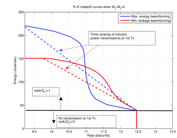
Figure 2: R-E tradeoff curves for MEB and MLB when $M=4$, $\alpha_{ii}=1$ for $i=1,2$, and $\alpha_{ij}=0.8$ for $i\neq j$.

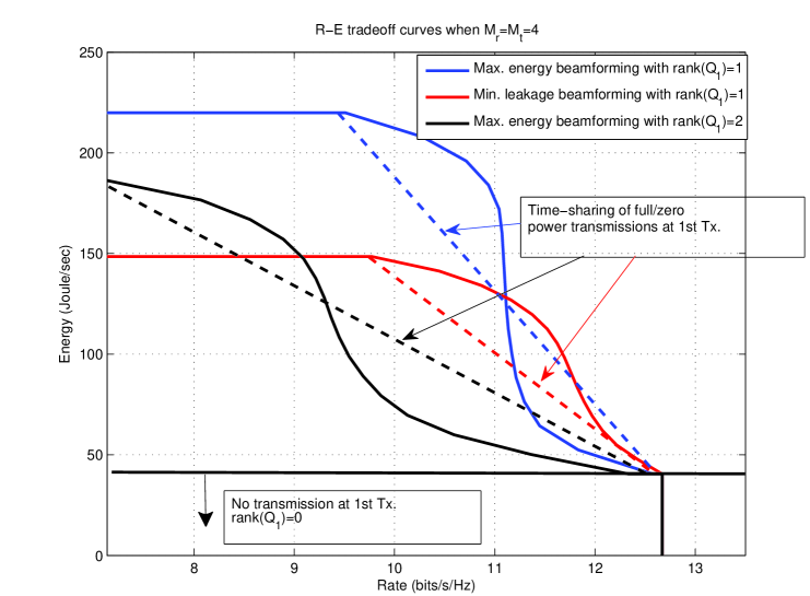
Figure 3: R-E tradeoff curves for MEBs ($rank({\bf Q}_{1})=\{1,2\}$) and MLB ($rank({\bf Q}_{1})=1$) when $M=4$, $\alpha_{ii}=1$ for $i=1,2$, and $\alpha_{ij}=0.8$ for $i\neq j$.

In Fig. 4, we plot R-E tradeoff curves for $M=4$ and $P=0.1$. As observed in Section VI-A, at the low SNR, the MEB exhibits higher harvested energy than the MLB without any degradations in the achievable rate. Fig. 5 shows R-E tradeoff curves for $M=15$. Compared to $M\in 4$ (Fig. 2), the gap between the achievable rates of MEB and MLB is relatively less apparent. As pointed out in Remark 3 of Section VI, for low SNRs or large numbers of antennas in the MIMO IFC, the energy transfer strategy of maximizing the transferred energy on its own link exhibits wider R-E region than that of minimizing the interference to the other ID receiver.

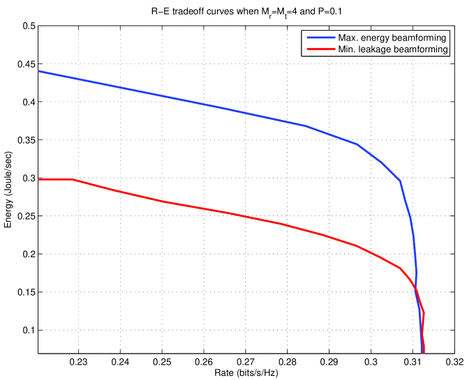
Figure 4: R-E tradeoff curves for MEB and MLB when $M=4$ and $P=0.1$.

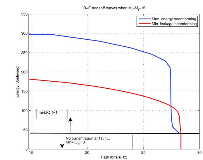
Figure 5: R-E tradeoff curves for MEB and MLB when $M=15$.

Fig. 6 shows R-E tradeoff curves for MEB, MLB, SLNR maximizing beamforming, and SLER maximizing beamforming when $M=4$, $\alpha_{ii}=1$ for $i=1,2$, and $\alpha_{ij}=0.8$ for $i\neq j$. The R-E region of the proposed SLER maximizing beamforming covers most of those of both MEB and MLB, while the SLNR beamforming does not cover the region for MEB. Fig. 7 shows R-E tradeoff curves for an asymmetric case $M_{t}=3$ and $M_{r}=4$. We can find a similar trend with $M_{t}=4=M_{r}=4$, but the overall harvested energy with $M_{t}=3$ and $M_{r}=4$ is slightly less than that with $M_{t}=4=M_{r}=4$.

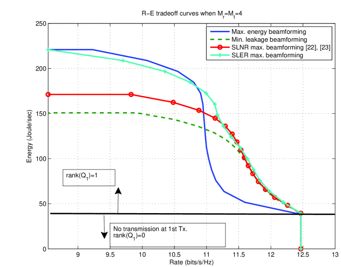
Figure 6: R-E tradeoff curves for MEB, the MLB, SLNR maximizing beamforming, and SLER maximizing beamforming when $M=4$, $\alpha_{ii}=1$ for $i=1,2$, and $\alpha_{ij}=0.8$ for $i\neq j$.

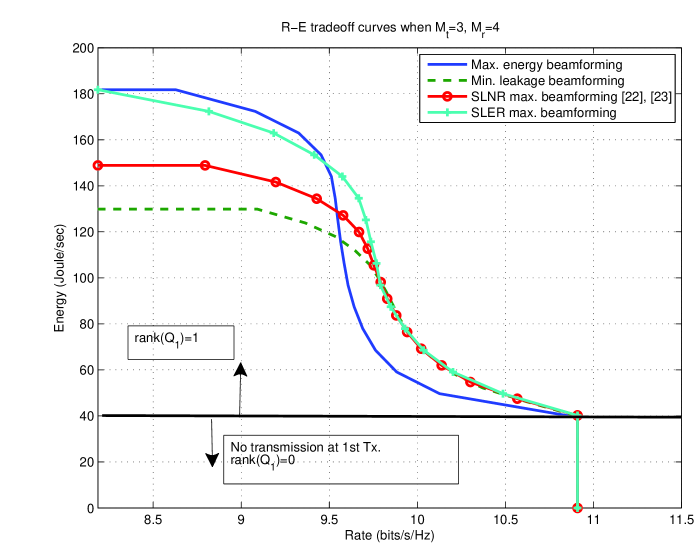
Figure 7: R-E tradeoff curves for MEB, the MLB, SLNR maximizing beamforming, and SLER maximizing beamforming when $M_{t}=3$ and $M_{r}=4$.

Fig. 8 shows the R-E tradeoff curves for SLER maximizing beamforming with/without SLER-based scheduling described in Section V when (a) $\alpha_{ij}=0.7$ and (b) $\alpha_{ij}=1$ for $i\neq j$. Here, we set $\alpha_{ii}=1$ for $i=1,2$ and $M=2$. Note that the case with $\alpha_{ij}=0.7$ has weaker cross-link channel (inducing less interference) than that with $\alpha_{ij}=1$. The SLER-based scheduling extends the achievable R-E region for both $\alpha_{ij}\in\{0.7,1\}$, but the improvement for $\alpha_{ij}=1$ is slightly more apparent. That is, the SLER-based scheduling becomes more effective when strong interference exists in the system. Note that the case with $\alpha_{ij}=1$ exhibits slightly lower achievable rate than that with $\alpha_{ij}=0.7$, while achieving larger harvested energy. That is, the strong interference degrades the information decoding performance but it can be effectively utilized in the energy-harvesting.

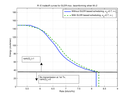
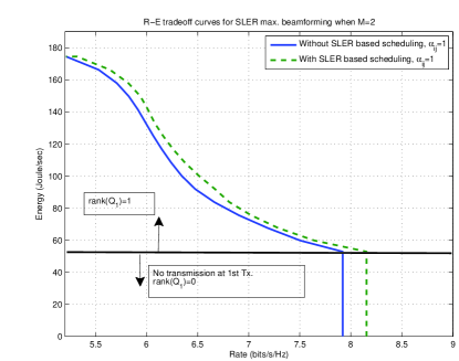
Figure 8: R-E tradeoff curves for SLER maximizing beamforming with/without SLER-based scheduling when (a) $\alpha_{ij}=0.7$ and (b) $\alpha_{ij}=1$ for $i\neq j$. Here, $M=2$.

VIII Conclusion

In this paper, we have investigated the joint wireless information and energy transfer in two-user MIMO IFC. Based on Rx mode, we have different transmission strategies. For single-operation modes - ($ID_{1}$, $ID_{2}$) and ($EH_{1}$, $EH_{2}$), the iterative water-filling and the energy-maximizing beamforming on both receivers can be adopted to maximize the information bit rate and the harvested energy, respectively. For ($EH_{1}$, $ID_{2}$), and ($ID_{1}$, $EH_{2}$), we have found a necessary condition of the optimal transmission strategy that one of transmitters should take a rank-one beamforming with a power control. Accordingly, for two transmission strategies that satisfy the necessary condition - MEB and MLB, we have identified their achievable R-E tradeoff regions, where the MEB (MLB) exhibits larger harvested energy (achievable rate). We have also found that when the SNR decreases or the number of antennas increases, the joint information and energy transfer in the MIMO IFC can be naturally split into disjoint information and energy transfer in two non-interfering links. Finally, we have proposed a new transmission strategy satisfying the necessary condition - signal-to-leakage-and-energy ratio (SLER) maximization beamforming which shows wider R-E region than the conventional transmission methods. That is, we have found that even though the interference degrades the ID performance in the two-user MIMO IFC, the proposed SLER maximization beamforming scheme effectively utilizes it in the EH without compromising ID performance.

Note that, motivated from the rank-one beamforming optimality, the identification of the optimal R-E boundary will be a challenging future work. Furthermore, the partial CSI or erroneous channel information degrades the achievable rate and the harvested energy at the receivers, which drives us to develop a robust rank-one beamforming.

References

- [1] A. Kurs, A. Karalis, R. Moffatt, J. D. Joannopoulos, P. Fisher, and M. Soljacic, “Wireless power transfer via strongly coupled magnetic resonances,” Science, vol. 137, no. 83, pp. 83–86, Sept. 2007.
- [2] M. Pinuela, D. Yates, S. Lucyszyn, and P. Mitcheson, “Maximizing DC-load efficiency for semi-resonant inductive power transfer,” submitted to IEEE Transactions on power electronics, 2012.
- [3] R. J. M. Vullers, R. V. Schaijk, I. Doms, C. V. Hoof, and R. Merterns, “Micropower energy harvesting,” Solid-State Electronics, vol. 53, no. 7, pp. 684–693, July 2009.
- [4] T. Le, K. Mayaram, and T. Fiez, “Efficient far-field radio frequency energy harvesting for passively powered sensor networks,” IEEE J. Solid-State Circuits, vol. 43, no. 5, pp. 1287–1302, May 2008.
- [5] O. Ozel, K. Tutuncuoglu, J. Yang, S. Ulukus, and A. Yener, “Transmission with energy harvesting nodes in fading wireless channels: Optimal policies,” IEEE J. Select. Areas Commun., vol. 29, no. 8, pp. 1732–1743, Sept. 2011.
- [6] R. Rajesh, V. Sharma, and P. Viswanath, “Information capacity of energy harvesting sensor nodes,” in Proc. IEEE International Symposium on Information Theory, 2011, July 2011, pp. 2363–2367.
- [7] ——, “Information capacity of an energy harvesting sensor node,” submitted to IEEE Transactions on Information Theory, http://arxiv.org/abs/1212.3177, 2012.
- [8] K. Ishibashi, H. Ochiai, and V. Tarokh, “Energy harvesting cooperative communications,” in Proc. IEEE International Symposium on Personal, Indoor and Mobile Radio Communications, 2012, Sept. 2012, pp. 1819–1823.
- [9] Y. Luo, J. Zhang, and K. B. Letaief, “Optimal scheduling and power allocation for two-hop energy harvesting communication systems,” submitted to IEEE Transactions on Wireless Communications, http://arxiv.org/abs/1212.5394, 2012.
- [10] R. Zhang and C. K. Ho, “MIMO broadcasting for simultaneous wireless information and power transfer,” submitted to IEEE Transactions on Wireless Communications, http://arxiv.org/abs/1105.4999, 2011.
- [11] L. Liu, R. Zhang, and K. Chua, “Wireless information transfer with opportunistic energy harvesting,” submitted to IEEE Transactions on Wireless Communications, http://arxiv.org/abs/1204.2035, 2012.
- [12] K. Huang and E. G. Larsson, “Simultaneous information-and-power transfer for broadband downlink systems,” submitted to IEEE ICASSP 2013, http://arxiv.org/abs/1211.6868, 2012.
- [13] A. A. Nasir, X. Zhou, S. Durrani, and R. A. Kennedy, “Relaying protocols for wireless energy harvesting and information processing,” submitted to IEEE Transactions on Wireless Communications, http://arxiv.org/abs/1212.5406, 2012.
- [14] K. Tutuncuoglu and A. Yener, “Sum-rate optimal power policies for energy harvesting transmitters in an interference channel,” Journal of Communications and Networks, vol. 14, no. 2, pp. 151–161, Apr. 2012.
- [15] ——, “Transmission policies for asymmetric interference channels with energy harvesting nodes,” in Proc. IEEE International Workshop on Computational Advances in Multi-sensor Adaptive Processing, 2011, Dec. 2011, pp. 197–200.
- [16] K. Huang and V. K. N. Lau, “Enabling wireless power transfer in cellular networks: architecture, modeling and deployment,” submitted to IEEE Transactions on Signal Processing, http://arxiv.org/abs/1207.5640, 2012.
- [17] X. Zhou, R. Zhang, and C. K. Ho, “Wireless information and power transfer: architecture design and rate-energy tradeoff,” submitted to IEEE Transactions on Communications, http://arxiv.org/abs/1205.0618, 2012.
- [18] C. Shen, W. Li, and T. Chang, “Simultaneous information and energy transfer: A two-user MISO interference channel case,” in Proc. IEEE GLOBECOM, 2012, Dec. 2012.
- [19] G. Scutari, D. P. Palomar, and S. Barbarossa, “The MIMO iterative waterfilling algorithm,” IEEE Trans. Signal Processing, vol. 57, no. 5, pp. 1917–1935, May 2009.
- [20] W. Yu, W. Rhee, S. Boyd, and J. M. Cioffi, “Iterative water-filling for gaussian vector multiple-access channels,” IEEE Trans. Inform. Theory, vol. 50, no. 1, pp. 145–152, Jan. 2004.
- [21] A. Goldsmith, S. A. Jafar, N. Jindal, and S. Vishwanath, “Capacity limits of MIMO channels,” IEEE J. Select. Areas Commun., vol. 21, no. 5, pp. 684–702, June 2003.
- [22] M. Sadek, A. Tarighat, and A. H. Sayed, “A leakage-based precoding scheme for downlink multi-user MIMO channels,” IEEE Trans. Wireless Commun., vol. 6, no. 5, pp. 1711–1721, May 2007.
- [23] J. Park, J. Chun, and H. Park, “Generalised singular value decomposition-based algorithm for multi-user MIMO linear precoding and antenna selection,” IET Commun., vol. 4, no. 16, pp. 1899–1907, Nov. 2010.
- [24] S. L. Loyka, “Channel capacity of MIMO architecture using the exponential correlation matrix,” IEEE Commun. Lett., vol. 5, no. 9, pp. 369–371, Sept. 2001.
- [25] C. C. Paige and M. A. Saunders, “Towards a generalized singular value decomposition,” SIAM Journal on Numerical Analysis, vol. 18, no. 3, pp. 398–405, June 1981.
- [26] D. A. Harville, Matrix algebra from a statistician’s perspective. Berlin: Springer, 2008.
- [27] R. A. Horn, N. H. Rhee, and W. So, “Eigenvalue inequalities and equalities,” Linear Algebra and Its Applications, vol. 270, no. 1-3, pp. 29–44, Feb. 1998.
- [28] V. R. Cadambe and S. A. Jafar, “Interference alignment and degrees of freedom of the K-user interference channel,” IEEE Trans. Inform. Theory, vol. 54, no. 8, pp. 3425–3441, Aug. 2008.
- [29] S. Boyd and L. Vandenberghe, Convex Optimization, 7th ed. New York: Cambridge University Press, 2009.
- [30] T. M. Cover and J. A. Thomas, Elements of Information Theory, 2nd ed. New Jersey: John & Sons, Inc., 2006.
- [31] X. Zhao, P. B. Luh, and J. Wang, “Surrogate gradient algorithm for Lagrangian relaxation,” Journal of Optimization Theory and Applications, vol. 100, no. 3, pp. 699–712, Mar. 1999.
- [32] J. Park, J. Chun, and B. Jeong, “Efficient multi-user MIMO precoding based on GSVD and vector perturbation,” Signal Processing, vol. 92, no. 2, pp. 611–615, Feb. 2012.
- [33] R. H. Gohary, W. Mesbah, and T. N. Davidson, “Rate-optimal MIMO transmission with mean and covariance feedback at low SNRs,” IEEE Trans. Veh. Technol., vol. 58, no. 7, pp. 3802–3807, Sept. 2009.
- [34] S. A. Jafar and A. Goldsmith, “Transmitter optimization and optimality of beamforming for multiple antenna systems,” IEEE Trans. Wireless Commun., vol. 3, no. 4, pp. 1165–1175, July 2004.
- [35] T. L. Marzetta, “Noncooperative cellular wireless with unlimited numbers of base station antennas,” IEEE Trans. Wireless Commun., vol. 9, no. 11, pp. 3590–3600, Nov. 2010.
- [36] J. Hoydis, S. T. Brink, and M. Debbah, “Massive MIMO: How many antennas do we need?” in Proc. Annual Allerton Conference on Communication, Control, and Computing, 2011, Sept. 2011, pp. 545–550.
- [37] F. Rusek, D. Persson, B. K. Lau, E. G. Larsson, T. L. Marzetta, O. Edfors, and F. Tufvesson, “Scaling up MIMO: opportunities and challenges with very large arrays,” IEEE Signal Processing Mag., vol. 30, no. 1, pp. 40–60, Jan. 2013.
- [38] A. Papoulis and S. U. Pillai, Probability, Random Variables and Stochastic Processes, 4th ed. Boston: McGraw-Hill, 2002.