Quantum states of the bouncing universe

Abstract

In this paper we study quantum dynamics of the bouncing cosmological model. We focus on the model of the flat Friedman-Robertson-Walker universe with a free scalar field. The bouncing behavior, which replaces classical singularity, appears due to the modification of general relativity along the methods of loop quantum cosmology. We show that there exist a unitary transformation that enables to describe the system as a free particle with Hamiltonian equal to canonical momentum. We examine properties of the various quantum states of the Universe: boxcar state, standard coherent state, and soliton-like state, as well as Schrödinger’s cat states constructed from these states. Characteristics of the states such as quantum moments and Wigner functions are investigated. We show that each of these states have, for some range of parameters, a proper semiclassical limit fulfilling the correspondence principle. Decoherence of the superposition of two universes is described and possible interpretations in terms of triad orientation and Belinsky-Khalatnikov-Lifshitz conjecture are given. Some interesting features regarding the area of the negative part of the Wigner function have emerged.

I Introduction

It is known that the cosmological singularity problem of the Friedman-Robertson-Walker (FRW) universe can be resolved, in the sense that big bang may be replaced by big bounce, by applying loop quantum cosmology (LQC) methods. However, quantum states specifying quantum evolution of the universe have not been examined in a satisfactory way yet.

There exist two alternative forms of LQC: Dirac’s LQC (see e.g. Ashtekar:2011ni ; Bojowald:2006da and references therein) and reduced phase space (RPS) LQC (see e.g. Dzierzak:2009ip ; Malkiewicz:2009qv ; Mielczarek:2011mx ; Mielczarek:2012qs ) and references therein). Both approaches rely on the same form of modification of general relativity. It consists in approximating the curvature of connection by holonomies around small loops with non-zero size. Going with the size to zero removes the modification. One of the main differences between these two approaches is an interpretation of the way of resolving the singularity. In the Dirac LQC, one argues that the resolution is due to strong quantum effects at the Planck scale. In the RPS LQC, one says that it is the modification of GR by loop deformation of the phase space that is responsible for the resolution of the singularity.

In what follows we apply the RPS LQC method. It consists in first solving dynamical constraints at the classical level and then quantizing the resulting classical system. This approach allows to implement quantization easily. It gives a clear picture of quantum dynamics for any value of an evolution parameter (time), and enables obtaining analytical results (at least for the FRW case).

The quantum evolution across the big bounce can give an insight into the structure of the quantum phase. The input in describing an evolution is a self-adjoint Hamiltonian (generator of dynamics) together with an initial state of the universe. Taking different initial states may lead to different quantum evolutions. Since it is unknown which initial state is the most natural one, we examine generic states known in quantum physics with different properties. Comparison of obtained results with observational cosmological data may give suggestions concerning the choice of some realistic initial state.

The paper is organized as follows. In Sec. II the classical dynamics of the model is examined and the canonical transformation simplifying the dynamics is introduced. In Sec. III we make canonical quantization of the model. We also introduce unitary map which corresponds to the canonical transformation introduced in Sec. II. In Sec. IV different choices of the initial quantum state are introduced as well as all the necessary tools which will be used to investigate their properties. Thereafter, in Sections V, VI and VII, detailed analysis of the boxcar state, standard coherent state, soliton-like state as well as Schrödinger cat states constructed from these states is performed. In Sec. VIII, decoherence of the Schrödinger cat state is discussed, and possible interpretations of such a process in the cosmological realm are given. The issue of quantum entropy is discussed Sec. IX. It is shown that, in contrast to the results of Ref. Mielczarek:2012qs , entropy of squeezing is constant for the canonically transformed system. Then, in Sec. X, ranges of the parameters of considered states are constrained by using the correspondence principle between quantum and classical mechanics. In Sec. XI, we summarize our results and draw conclusions.

II Classical dynamics

The flat FRW model of the universe with a free scalar field is described by the Hamiltonian constraint Mielczarek:2011mx

$$\tilde{H}=-\frac{3}{8\pi G\gamma^{2}}\frac{\sin^{2}(\lambda\beta)}{\lambda^{2}}v+\frac{p^{2}_{\varphi}}{2v}\approx 0,$$ (1)

where, as in the rest of this paper, we use the units with the speed of light in vacuum equal to one. Here, $\gamma$ is the Barbero-Immirzi parameter, a free parameter of the theory. However, value of this parameter is usually fixed from considerations of the black hole entropy. In particular, as derived in Ref. Meissner:2004ju , $\gamma\approx 0.2375$. The parameter $\lambda$ is a ‘discretization scale’, which is expected to be of the order of the Planck length $l_{\text{Pl}}=\sqrt{\hslash G}\approx 1.62\cdot 10^{-35}$ m, but in fact should be fixed by observational data.

The variables $\beta$ and $v$, fulfilling the Poisson bracket $\{\beta,v\}=4\pi G\gamma$, parametrize the gravitational sector. In turn, the scalar field $\varphi$ and its conjugated momenta $p_{\varphi}$ satisfy standard relation $\{\varphi,p_{\varphi}\}=1$, and specify sources.

Hamiltonian (1) has the symmetry

$$\beta\rightarrow\beta+\frac{\pi}{\lambda},$$ (2)

so the gravitational part of phase space has topology of a cylinder, $S^{1}\times\mathbb{R}$. Already classically we have bounce type solutions in the regions: $\lambda\beta\in[0+m\pi,\pi+m\pi]$, for $m\in\mathbb{Z}$.

The Hamiltonian constraint (1) can be rewritten in the form

$$v^{2}\sin^{2}(\lambda\beta)=\text{const},$$ (3)

where we used the fact that $p_{\varphi}=$ const for the free field case. It turns, that the square root of (3) plays a role of the physical Hamiltonian. Based on this, dynamics of a flat FRW cosmological model, with a freescalar field, can be described by

$$H=p\ \sin q,$$ (4)

where $q\in[0,\pi]$ and $p\in\mathbb{R}$ are canonical variables satisfying the algebra $\{q,p\}=1$. The Hamiltonian (4) occurs both in the reduced phase space approach Mielczarek:2011mx and standard formulation of LQC Bojowald:2007zza . It need not be bounded from below as it describes the entire universe, which is an isolated system. The $p$ variable is proportional to the volume $v$, but we increase its range to negative values for mathematical convenience. Physical meaning of this volume is not clear for the flat FRW model. It corresponds to the total volume of space if topology is compact. The possibility of positive and negative values of $p$ may be related to two orientations of triad. Namely, the phase space $(\beta,v)$ is only half of the original phase space of the model since $v:=\left|\tilde{p}V_{0}^{2/3}\right|^{3/2}$, where $\bar{p}\in\mathbb{R}$ is a variable parametrizing densitized triad $E^{{}^{a}_{i}}=\tilde{p}\delta^{a}_{i}$. The $V_{0}$ is a fiducial cell over which the spatial integration is performed. By allowing positive and negative values of the variable $p$ we recover the volume of the original phase space. The variable $q:=\lambda\beta$ is proportional to the Hubble factor in the classical limit ($q\ll 1$).

The Hamiltonian (4) generates evolution of any phase space function $f$ according to the equation

$$\frac{df}{dT}=\{f,H\}.$$ (5)

The $T$ variable is an intrinsic time parameter related with the value of the scalar field. The direction of time $T$, which also occurs in Mielczarek:2011mx , is opposite to the direction of the coordinate time $t$. In order to fix the directions of $T$ and $t$ one has to redefine $T$ by multiplying it and the Hamiltonian (4) by minus one. But these are only technical details devoid of deep meaning.

Applying (5) for the canonical variables we get

$$\frac{dq}{dT} = \frac{\partial H}{\partial p}=\sin q,$$ (6)

$$\frac{dp}{dT} = -\frac{\partial H}{\partial q}=-p\,\cos q.$$ (7)

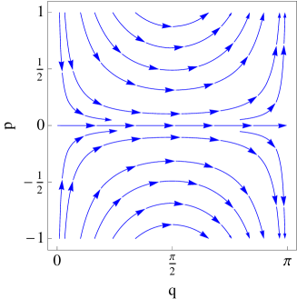
Figure 1: Trajectories in the phase space with original variables $(q,p)$.

Solutions to these equations are given by

$$q(T) = 2\arctan\exp(T-T_{0}),$$ (8)

$$p(T) = p_{0}\cosh(T-T_{0}),$$ (9)

where $p_{0}$ and $T_{0}$ are constants of integration. The solution for $p$ presents a nonsingular symmetric bounce type evolution. Fig. 1 presents the phase portrait of the phase space, illustrating Eqs. (8) and (9).

II.1 Canonical transformation

Let us define the map $(q,p)\in(0,\pi)\times\mathbb{R}\mapsto(Q,P)\in\mathbb{R}^{2}$ as follows:

$$Q := \log\tan\left(\frac{q}{2}\right)\in\mathbb{R},$$ (10)

$$P := p\ \sin(q)\in\mathbb{R}.$$ (11)

In contrast to $q$ and $p$, both new variables $Q$ and $P$ are defined on the entire real line. The variables $Q$ and $P$ fulfill the following Poisson bracket

$$\left\{Q,P\right\}=\frac{\partial Q}{\partial q}\frac{\partial P}{\partial p}-\frac{\partial Q}{\partial p}\frac{\partial P}{\partial q}=1,$$ (12)

so the transformation (10)-(11) is canonical.

In what follows we use the following identities

$$\sin q=\frac{1}{\cosh Q},~{}~{}~{}~{}\frac{dQ}{dq}=\frac{1}{\sin q}=\cosh Q,$$ (13)

which are useful in further considerations.

In the new variables the Hamiltonian (4) reads

$$H=P,$$ (14)

which resembles the Hamiltonian of photon. The equations of motion are:

$$\frac{dQ}{dT} = \frac{\partial H}{\partial P}=1,$$ (15)

$$\frac{dP}{dT} = -\frac{\partial H}{\partial Q}=0,$$ (16)

which have the solutions

$$Q(T)=T+c_{1},~{}~{}~{}~{}P(T)=c_{2},$$ (17)

where $c_{1}$ and $c_{2}$ are constants of integration. The corresponding phase portrait composes of the parallel trajectories, as shown in Fig. 2.

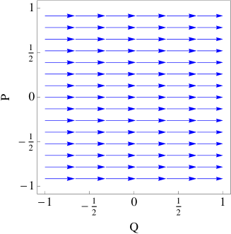
Figure 2: Trajectories in the phase space $(Q,P)$.

Comparing Figs. 1 and 2 we can see the importance of making suitable choice of phase space variables. The simplification in describing the dynamics is manifest.

III Quantum dynamics

In order to quantize the system, we introduce the Hilbert space $\mathcal{H}_{1}=L^{2}([0,\pi],dq)$. In the Dirac LQC, one considers the Bohr Hilbert space of almost periodic functions, instead of the $L^{2}$ space, which complicates quantization.

The action of the operators $\hat{q}$ and $\hat{p}$ is defined as follows

$$\hat{q}\phi = q\phi,$$ (18)

$$\hat{p}\phi = -i\hslash\frac{d}{dq}\phi.$$ (19)

The presence of the symbol $\hslash$ is justified by the physical dimension of variable $p$ which is an action in the units we have chosen from the beginning (time has no dimension, and $p$ is energy-like). While passing from classical to quantum theory, along canonical quantization procedure, the known problem of factor ordering appears. In our case we have

$$H=p\;\sin q=\left(\sin q\right)^{n}p\;\left(\sin q\right)^{1-n}=:H_{n},$$ (20)

which can be quantized as follows (letting aside the formal appearance of singularities)

$$\hat{H}_{n}:=\frac{1}{2}\left[\left(\sin\hat{q}\right)^{n}\widehat{p}\left(\sin\hat{q}\right)^{1-n}+\left(\sin\hat{q}\right)^{1-n}\widehat{p}\left(\sin\hat{q}\right)^{n}\right],$$ (21)

where $n\in\mathbb{R}$.

For such a class of possible factor orderings, the resulting Hamiltonian takes the following form

$$\hat{H}_{n}\phi=-i\hslash\left[\frac{1}{2}\cos q+\sin q\frac{d}{dq}\right]\phi=:\hat{H}\phi,$$ (22)

so in a sense it does not depend on $n$. In some cases, however, it is advantageous to make some specific choice. The case $n=1$ was used in Ref. Mielczarek:2011mx , while $n=1/2$ is considered in what follows. The latter choice is useful while defining an isometry transformation.

III.1 Eigenfunctions

The eigenequation of the Hamilton operator is the following

$$-i\hslash\left[\frac{1}{2}\cos(q)\phi+\sin(q)\frac{d\phi}{dq}\right]=E\phi,$$ (23)

where $E\in\mathbb{R}$ belongs to the continuous spectrum. Solution to this equation is given by

$$\phi_{E}(q)=\frac{1}{\sqrt{2\pi\hslash}}\frac{\exp\left\{\frac{i}{\hslash}E\ln\tan\left(\frac{q}{2}\right)\right\}}{\sqrt{\sin q}}.$$ (24)

One can verify that

$$\langle\phi_{E_{1}}|\phi_{E_{2}}\rangle = \int_{0}^{\pi}\overline{\phi_{E_{1}}(q)}\phi_{E_{2}}(q)dq$$ (25)

$$= \frac{1}{2\pi\hslash}\int_{0}^{\pi}dq\frac{\exp\left\{\frac{i}{\hslash}(E_{2}-E_{1})\ln\tan\left(\frac{q}{2}\right)\right\}}{\sin q}$$

$$= \frac{1}{2\pi\hslash}\int_{-\infty}^{+\infty}dQe^{\frac{i}{\hslash}(E_{2}-E_{1})Q}$$

$$= \delta(E_{2}-E_{1}),$$

where we have used the mapping (10)

$$(0,\pi)\ni q\rightarrow Q(q)\in\mathbb{R}.$$ (26)

III.2 Unitary map

For $n=1/2$, the quantum Hamiltonian reads

$$\hat{H}:=\sqrt{\sin\hat{q}}\ \widehat{p}\ \sqrt{\sin\hat{q}}.$$ (27)

Now, we introduce a new Hilbert space $\mathcal{H}_{2}=L^{2}(\mathbb{R},dQ)$ connected with $\mathcal{H}_{1}$ as follows

$$\mathcal{U}:\ \phi(q)\in\mathcal{H}_{1}\rightarrow\psi(Q)=\sqrt{\sin(q(Q))}\phi(q(Q))\in\mathcal{H}_{2}.$$ (28)

In particular, the eigenfunctions $\phi_{E}(q)$ are mapped into the plane waves

$$\mathcal{U}:\ \phi_{E}(q)\rightarrow\psi_{E}(Q)=\frac{e^{\frac{i}{\hslash}EQ}}{\sqrt{2\pi\hslash}}.$$ (29)

The map $\mathcal{U}$ is an invertible isometry (unitary transform), since we have

$$\langle\phi_{1}|\phi_{2}\rangle_{\mathcal{H}_{1}} = \int_{0}^{\pi}\overline{\phi_{1}(q)}\phi_{2}(q)dq$$ (30)

$$= \int_{-\infty}^{+\infty}\overline{\phi_{1}(q(Q))}\phi_{2}(q(Q))\sin(q(Q))dQ$$

$$= \int_{-\infty}^{+\infty}\overline{\psi_{1}(Q)}\psi_{2}(Q)dQ=\langle\psi_{1}|\psi_{2}\rangle_{\mathcal{H}_{2}}.$$

Under this isometry, an operator $\hat{O}_{\mathcal{H}_{1}}$ acting in $\mathcal{H}_{1}$ is transformed into an operator $\hat{O}_{\mathcal{H}_{2}}$ acting on $\mathcal{H}_{2}$ and vice versa

$$\hat{O}_{\mathcal{H}_{2}} = \mathcal{U}\hat{O}_{\mathcal{H}_{1}}\mathcal{U}^{-1},$$ (31)

$$\hat{O}_{\mathcal{H}_{1}} = \mathcal{U}^{-1}\hat{O}_{\mathcal{H}_{2}}\mathcal{U}.$$ (32)

As an example, let us consider the operator $\hat{P}$ which acts in $\mathcal{H}_{2}$ as follows

$$\hat{P}\psi(Q)=-i\hslash\frac{d}{dQ}\psi(Q).$$ (33)

Using the transformation (32) as well as relation (13), we obtain

$$\hat{P}\psi(Q) = \mathcal{U}^{-1}\hat{P}\mathcal{U}\phi(q)=\frac{1}{\sqrt{\sin q}}\left(-i\hslash\frac{d}{dQ}\right)\sqrt{\sin q}\phi(q)$$ (34)

$$= \frac{1}{\sqrt{\sin q}}\left(-i\hslash\sin q\frac{d}{dq}\right)\sqrt{\sin q}\phi(q)$$

$$= \sqrt{\sin q}\left(-i\hslash\frac{d}{dq}\right)\sqrt{\sin q}\phi(q)$$

$$= \widehat{\sqrt{\sin q}}\ \widehat{p}\ \widehat{\sqrt{\sin q}}\phi(q)$$

$$= \hat{H}\phi(q).$$

Thus, the isometry $\mathcal{U}$ transforms the Hamiltonian $\hat{H}$ acting in $\mathcal{H}_{1}$ into a well known momentum operator $\hat{P}$ acting in $\mathcal{H}_{2}$.

Using the above results, we define a unitary evolution operator $\hat{U}$ as follows:

$$\hat{U}\phi(q):=e^{-\frac{i}{\hslash}\hat{H}T}\phi(q)=e^{-\frac{i}{\hslash}\hat{P}T}\psi(Q)$$

$$=\exp\left\{-T\frac{d}{dQ}\right\}\psi(Q)=\psi(Q-T).$$ (35)

Therefore, a time evolution in $\mathcal{H}_{1}$ corresponds to translation operator in $\mathcal{H}_{2}$. So the shape of the probability distribution is preserved in time.

The classical dynamics of the $Q$ variable is $Q=T+c_{1}$ (See Eq. 17). Thus, if the probability distribution is peaked on the classical trajectory at some given moment in time, it will trace the classical trajectory during the whole evolution Zipfel .

We should notice at this point that combining translation (III.2) with phase modulation, $\Psi(Q)\mapsto e^{\frac{i}{\hslash}P_{0}Q}\Psi(Q):=\Psi_{P_{0}}(Q)$, leads to the unitary irreducible representation of the Weyl-Heisenberg group

$$\Psi(Q)\mapsto e^{\frac{i}{\hslash}P_{0}Q}\Psi(Q-T):=\Psi_{P_{0},T}(Q)\,,$$ (36)

used for constructing coherent states in quantum mechanics (up to a constant phase factor) perelomov86 ; gazeaubook09 and the Gabor states for time-frequency analysis used in signal processing walkerbook08 . The Weyl-Heisenberg action (36) will be at the heart of the construction of the examples presented in the next section.

IV Choice of initial state

In the next three sections we investigate three representative initial quantum states:

• Boxcar state

• Standard coherent state

• Soliton-like state

Moreover, for each of these states we investigate Schrödinger cat type superposition in the form

$$\Psi=\frac{N}{\sqrt{2}}\left(\Psi_{P_{0}}+\Psi_{-P_{0}}\right)\,$$ (37)

where $P_{0}$ is the mean value of the $\hat{P}$ operator in the constituent state $\Psi_{P_{0}}$ and $N$ is the normalization factor. It is known that such states are experimentally attainable (for instance in quantum optics grangieretal07 ). The state (see Sec. 69) can be viewed also as a superposition of the two orientations of triads. Decoherence of two triads orientations in LQC was recently studied in Ref. Kiefer:2012kp . In what follows we study such a process in our framework.

As was already mentioned, quantum dynamics of the considered model reduces to shifting the initial state in the $Q$ variable: $\hat{U}(T)\Psi(Q)=\Psi(Q-T)$. Therefore while we have the initial quantum state $\Psi(Q)$, the corresponding state at the time $T$ is obtained by replacing $Q\rightarrow Q-T$. For the later convenience we define variable $X:=Q-T$, which absorbs all time dependence of a given quantum state.

To characterize the states under consideration we study quantum moments of the operators $\hat{Q}$ and $\hat{P}$ in the given state. In particular, determination of the mean values $\langle\hat{Q}\rangle$ and $\langle\hat{P}\rangle$ is crucial to compare quantum dynamics with the classical phase-space trajectories. Furthermore, quantum dispersions

$$\sigma_{Q}:=\sqrt{\langle\hat{Q}^{2}\rangle-\langle\hat{Q}\rangle^{2}},~{}~{}~{}~{}\sigma_{P}:=\sqrt{\langle\hat{P}^{2}\rangle-\langle\hat{P}\rangle^{2}},$$ (38)

as well as covariance

$$C_{QP}:=\langle(\hat{Q}-\langle\hat{Q}\rangle)(\hat{P}-\langle\hat{P}\rangle)\rangle$$

$$=\frac{1}{2}\langle\hat{Q}\hat{P}+\hat{P}\hat{Q}\rangle-\langle\hat{Q}\rangle\langle\hat{P}\rangle,$$ (39)

will be a source of information about spreading and squeezing of the quantum states. Furthermore, by employing dispersions and covariance, one can define the covariance matrix

$${\bf\Sigma}:=\left[\begin{array}[]{cc}\sigma_{Q}^{2}&C_{QP}\\ C_{QP}&\sigma_{P}^{2}\end{array}\right].$$ (40)

Making use of it, one can define the Schrödinger-Robertson uncertainty relation as follows

$$\det{\bf\Sigma}\geq\frac{\hslash^{2}}{4}.$$ (41)

The value of $\det{\bf\Sigma}$ is an important characteristic of the quantum state, telling us about spread of the state on the phase space. One could expect that for small values of $\det{\bf\Sigma}$, the quantum systems behaves more like a classical one. However, it is not a general rule. Therefore, other indicators of semi-classicality should be used.

In the literature, the relative fluctuations $\sigma_{\mathcal{O}}/\langle\hat{O}\rangle$ are usually considered as a measure of semi-classicality. Namely, one could expect that, in the semiclassical limit, quantum fluctuations of some observable $\hat{O}$ should be much smaller that its mean value: $\sigma_{\mathcal{O}}/\langle\hat{O}\rangle\ll 1$. Such a definition has to be however applied with care. Namely, while denominator $\langle\hat{O}\rangle$ approaches zero, the relative fluctuations diverge even, if the quantum dispersion is very small. But this does not correspond to any strong quantum effects, and is only a result of the definition of the observable $\hat{O}$. Another important aspect is the meaning of choosing $\sigma_{\mathcal{O}}/\langle\hat{O}\rangle$ being much smaller that one. Should it be one hundred or one million times smaller? While the choice is quite arbitrary, we already have a reference value coming from the measurements of a given observable. If our experimental abilities does not allow us to see the quantum aspects of a given phenomenon, then we can state that the underlying dynamics is classical. Therefore, the state can be called semiclassical if relative fluctuations of some observable are smaller than the relative uncertainty of experimental (observational) determination of that observable.

In what follows we study one quantity, which can be used to characterize semi-classicality of a quantum state. Namely, the Wigner function, which is a quasi-probability distribution defined on the phase space. Having the wave function $\Psi(Q)=\langle Q|\Psi\rangle$ of a pure state $|\Psi\rangle$, the Wigner function is defined to be

$$W(Q,P):=\frac{1}{\pi\hslash}\int_{-\infty}^{+\infty}\overline{\Psi}(Q+y)\Psi(Q-y)e^{2iPy/\hslash}dy.$$ (42)

The basic properties of the Wigner function are

$$\int_{-\infty}^{+\infty}\int_{-\infty}^{+\infty}W(Q,P)dQdP=1,$$ (43)

$$\int_{-\infty}^{+\infty}W(Q,P)dP=|\Psi(Q)|^{2},$$ (44)

$$\int_{-\infty}^{+\infty}W(Q,P)dQ=|\Psi(P)|^{2},$$ (45)

and

$$-\frac{1}{\pi\hslash}\leq W(Q,P)\leq\frac{1}{\pi\hslash}.$$ (46)

The last property tells us that also negative values of the the Wigner function are allowed. It was suggested that such negative part of the Wigner function can be considered as an indicator of quantumness Kenfeck2004 . Briefly, less negative the Wigner function is, more classically the system behaves. In this context the parameter $\delta(\Psi)$ was introduced in Ref. Kenfeck2004 :

$$\delta(\Psi):=\int_{-\infty}^{+\infty}\int_{-\infty}^{+\infty}|W(X,P)|dXdP-1\in[0,\infty].$$ (47)

One half of this parameter is equal to the modulus of the integral over those domains of the phase space where the Wigner function is negative.

One says that a state is semiclassical if $\delta(\Psi)\ll 1$.

In this paper, we study also areas of the negative parts of the Wigner functions for the considered states. This issue, as far as we know, was not systematically investigated yet. We show that the structure of these negative sectors may uncover some deep aspects of the formulation of quantum mechanics on phase space.

The Wigner function for the Schördinger cat state (see Sec. 69) can be written as the following sum

$$W(X,P)=\frac{N^{2}}{2}(W_{+}+W_{-})+W_{\text{int}},$$ (48)

where $W_{\pm}$ are Wigner functions for $\Psi_{\pm P_{0}}$ states while the interference term

$$W_{\text{int}} = \frac{N^{2}}{2\pi\hslash}\int_{-\infty}^{+\infty}\left[\overline{\Psi}_{P_{0}}(x+y)\Psi_{-P_{0}}(x-y)\right.$$ (49)

$$+ \left.\overline{\Psi}_{-P_{0}}(x+y)\Psi_{P_{0}}(x-y)\right]e^{2iPy/\hslash}dy.$$

Surprisingly for the considered states, including the Schrödinger cat states, it is possible to find analytical formulas for the corresponding Wigner functions. Plots of the Wigner functions will allow to better visualize some quantum aspects of the states.

V Boxcar state

V.1 Construction

We begin with considering the most basic example of a state with compact support, namely the rectangular or ‘boxcar’ window, widely used in Gabor signal analysis walkerbook08 . The definition of the state is the following

$$\Psi_{P_{0}}(Q)=\left\{\begin{array}[]{ccc}0&\text{for}&|Q|>\frac{L}{2}\\ \frac{1}{\sqrt{L}}e^{\frac{i}{\hslash}QP_{0}}&\text{for}&|Q|\leq\frac{L}{2}\end{array}\right.,$$ (50)

where $L>0$ (the dependence of $\Psi_{P_{0}}$ on parameter $L$ is not made explicit for the sake of simplicity). This state can be also written as

$$\Psi_{P_{0}}(Q)=\frac{1}{\sqrt{L}}e^{\frac{i}{\hslash}QP_{0}}\Theta\left(\frac{L}{2}+Q\right)\Theta\left(\frac{L}{2}-Q\right),$$ (51)

where $\Theta(x)$ is the Heaviside step function.

V.2 Quantum moments

The mean value and the dispersions of $\hat{Q}$ at the time $T$ are found to be

$$\langle\hat{Q}\rangle = T,$$ (52)

$$\sigma_{Q} = \frac{L}{\sqrt{12}}.$$ (53)

As expected from the previous analysis, evolution of the mean value $\langle\hat{Q}\rangle$ traces the classical dynamics. Here, the quantum dynamics correspond to the classical trajectory with the constant of integration $c_{1}=0$ (see Eq. (17).

Difficulties due to the discontinuous character of the considered state prevent the evaluation of a similar quantity for the momentum, since the computation of $\langle\hat{P}\rangle$ and $\langle\hat{P}^{2}\rangle$ involves divergent integrals. In principle, one can proceed with a regularization of these divergences, however the obtained expressions for $\langle\hat{P}\rangle$ and $\sigma_{P}$ would not have standard interpretation. Such results, are however of little use, and therefore not discussed here.

V.3 Wigner function

Based on definition (42), Wigner function for the boxcar state is

$$W(X,P)=\left\{\begin{array}[]{ccc}0&\text{for}&|X|>\frac{L}{2}\\ \frac{\sin\left[\dfrac{2(P-P_{0})}{\hslash}\left(\frac{L}{2}-|X|\right)\right]}{\pi L(P-P_{0})}&\text{for}&|X|\leq\frac{L}{2}\end{array}\right.$$ (54)

We plot this function in Fig. 3.

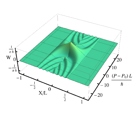
Figure 3: Wigner function for the boxcar state.

Furthermore, in Fig. 4, we show regions of the negative values of the Wigner function.

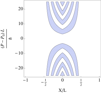
Figure 4: Regions where the Wigner function for the boxcar state assumes its negative values.

It is worth noticing that for $X=0$ and $P=P_{0}$ the Wigner function takes the maximal possible value:

$$W(0,P_{0})=\frac{1}{\pi\hslash}.$$ (55)

As we will see later, analysis of the Wigner functions suggests that

$$W(\langle\hat{X}\rangle,\langle\hat{P}\rangle)=\frac{1}{\pi\hslash}.$$ (56)

As far as we know such a relation was not proved so far. However, at least for the known Wigner functions it is always fulfilled. For the boxcar state, indeed $\langle\hat{X}\rangle=\langle\hat{Q}\rangle-T=T-T=0$, however the value of $\langle\hat{P}\rangle$ is not properly defined in the present case. However, since the obtained Wigner function is symmetric with respect to $P_{0}$, one can formally write $\langle\hat{P}\rangle=P_{0}$, supporting the relation (56).

V.4 Schrödinger cat state

The normalization factor for the Schrödinger cat state composed of two boxcar states is

$$N=\frac{1}{\sqrt{1+\frac{\sin(LP_{0}/\hslash)}{(LP_{0}/\hslash)}}}.$$ (57)

The interference part of the Wigner function is

$$W_{\text{int}}=\left\{\begin{array}[]{ccc}0&\text{for}&|X|>\frac{L}{2}\\ \dfrac{N^{2}\cos\left[\frac{2P_{0}X}{\hslash}\right]\sin\left[\frac{2P}{\hslash}\left(\frac{L}{2}-|X|\right)\right]}{\pi LP}&\text{for}&|X|\leq\frac{L}{2}\end{array}\right.$$ (58)

Plot of the Wigner function for the Schrödinger cat state composed of two boxcar states is shown in Fig. 5.

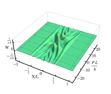
Figure 5: Wigner function of the Schrödinger cat state $LP_{0}=7\hslash$.

In Fig. 6 we show regions of the negative values of the Wigner function.

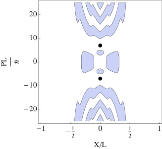
Figure 6: Regions where the Wigner function for the Schrödinger cat state assumes its negative values, with $LP_{0}=7\hslash$. The black dots represent peaks of the two constituent states.

For $LP_{0}\gtrsim 6.04$ there are two regions with negative values of the Wigner function, located at the $X=0$ axis. We observe that for the particularly case $LP_{0}=7\hslash$ the area of each of these regions is about $0.198\hbar$. However, while approaching the value $LP_{0}\approx 6.04$, the area of these regions falls to zero. At around $LP_{0}\gtrsim 7.64$ these two regions merge with the two negative domains located at $P=0$ axis.

VI Standard coherent state

VI.1 Construction

Standard or Glauber coherent states (see gazeaubook09 and references therein) are known to play a central role in studies of connection between classical and quantum world.

In quantum cosmology one expects that in the low energy density limit, the state is described by the coherent state mimicking the classical behavior. Here we study the state in which such a semi-classical behavior is preserved during the whole evolution. Namely, we consider a squeezed initial wave packet state like

$$\Psi_{0}(Q)=\int_{-\infty}^{+\infty}f(P)\psi_{P}(Q)dP,$$ (59)

where $\psi_{P}(Q)$ is the eigenstate of the $\hat{P}$ operator and

$$f(P)=\exp\left(-z_{1}P^{2}+z_{2}P+z_{3}\right),$$ (60)

where $z_{1},z_{2},z_{3}\in\mathbb{C}$, such that $\Re z_{1}>0$. The integral (59) is of the Gaussian type and can be calculated analytically. Due to (III.2) we get $\Psi(Q,T)=\hat{U}\Psi_{0}(Q)$ which finally reads

$$\Psi(Q,T)=\left(\frac{2\Re a_{1}}{\pi}\right)^{1/4}e^{-a_{1}(Q-T)^{2}+a_{2}(Q-T)-\frac{(\Re a_{2})^{2}}{4\Re a_{1}}}.$$ (61)

The factors $a_{1}$ and $a_{2}$ can be expressed in terms of coefficients $z_{1}$ and $z_{2}$ as follows

$$a_{1}:=\frac{1}{4\hslash^{2}z_{1}},~{}~{}~{}~{}~{}~{}a_{2}:=\frac{iz_{2}}{2\hslash z_{1}}.$$ (62)

It is worth stressing that the condition $\Re z_{1}>0$ enables normalization of the state.

VI.2 Quantum moments

The mean values of the canonical variables in the state (61) are found to be

$$\langle\hat{Q}\rangle=T+\underbrace{\frac{1}{2}\frac{\Re a_{2}}{\Re a_{1}}}_{=\ c_{1}\in\mathbb{R}},~{}~{}~{}~{}~{}~{}\langle\hat{P}\rangle=\underbrace{\hslash\left(\frac{\Im a_{2}}{\Im a_{1}}-\frac{\Re a_{2}}{\Re a_{1}}\right)\Im a_{1}}_{=\ c_{2}\in\mathbb{R}},$$ (63)

and are in agreement with the classical solutions (17). Furthermore, the dispersions are

$$\sigma_{Q}=\frac{1}{2\sqrt{\Re a_{1}}}$$ (64)

and

$$\sigma_{P}=\hslash\sqrt{\Re a_{1}}\sqrt{1+\left(\frac{\Im a_{1}}{\Re a_{1}}\right)^{2}}.$$ (65)

Finally, the covariance reads

$$C_{QP}=-\frac{\hslash}{2}\frac{\Im a_{1}}{\Re a_{1}}.$$ (66)

Based on the above, the determinant of the covariance matrix reads

$$\det{\bf\Sigma} = \sigma_{Q}^{2}\sigma_{P}^{2}-C_{QP}^{2}$$ (67)

$$= \frac{1}{4\Re a_{1}}\hslash^{2}\Re a_{1}\left[1+\left(\frac{\Im a_{1}}{\Re a_{1}}\right)^{2}\right]-\left(\frac{\hslash}{2}\frac{\Im a_{1}}{\Re a_{1}}\right)^{2}$$

$$= \frac{\hslash^{2}}{4}.$$

As expected for such a case, the squeezed state saturates the Schrödinger-Robertson uncertainty relation.

VI.3 Wigner function

For the standard coherent state, the Wigner function takes the form of the two dimensional Gauss distribution

$$W(X,P)=\frac{1}{\pi\hslash}\exp\left(-\frac{1}{2}{\bf x}^{T}{\bf\Sigma}^{-1}{\bf x}\right),$$ (68)

where ${\bf x}=(X-\langle\hat{X}\rangle,P-\langle\hat{P}\rangle)$. It is worth stressing, that the Wigner function (68) is positive definite. As Hudson-Piquet Hudson1974 theorem says, this is a characteristic property of the standard coherent states, distinguishing them among other pure states. Therefore, positiveness of the Wigner function can be treated as a definition of the standard coherent state. Taking negativeness of the Wigner function as a measure of the quantumness, one can conclude that the standard coherent states are the most classical pure states. Furthermore, the positivitiveness of the Wigner function is observed also for the mixed states Brocker1995 .

Plot of the Wigner function (68) is shown in Fig. 7.

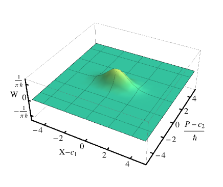
Figure 7: Wigner function for the standard coherent state. We set $C_{QP}=0$ and $\sigma_{Q}=1$, which implies $\sigma_{P}=\hslash/2$.

We set $C_{QP}=0$, thus axes of symmetry of the obtained Gaussian distribution overlap with the axes of coordinates. In the case of $C_{QP}\neq 0$ the distribution would rotate around the centre of the coordinate system.

VI.4 Schrödinger’s cat state

The standard coherent state can be interpreted as the least quantum state, since they saturate uncertainty relation during the whole evolution. However, by creating superposition of such states, strictly non-semiclassical states can be formed. Here, we study Schrödinger’s cat type superposition of two standard coherent states. For simplicity, we consider the case in which $\Re a_{1}=\frac{1}{4\hslash^{2}\alpha}$, $\Im a_{1}=0$, $\Re a_{2}=0$ and $\Im a_{2}=\frac{P_{0}}{\hslash}$. Taking this into account, the state (61) reduces to

$$\Psi_{P_{0}}(X)=\frac{1}{(2\pi\hslash^{2}\alpha)^{1/4}}e^{-\frac{X^{2}}{4\hslash^{2}\alpha}+\frac{i}{\hslash}P_{0}X}.$$ (69)

Based on this, we construct Schrödinger’s cat type superposition . The normalization factor in this case is

$$N=\frac{1}{\sqrt{1+\exp(-2P_{0}^{2}\alpha)}},$$ (70)

thus in the limit $P_{0}\rightarrow 0$ we get $N\rightarrow 1/\sqrt{2}$, so $\Psi\rightarrow\Psi_{P_{0}=0}$. The corresponding probability distribution function takes the form:

$$|\Psi(X)|^{2}=\frac{N^{2}e^{-\frac{X^{2}}{2\hslash^{2}\alpha}}}{\sqrt{2\pi\hslash^{2}\alpha}}\left[1+\cos\left(\frac{2P_{0}X}{\hslash}\right)\right].$$ (71)

The mean values of the canonical variables in the state (see Sec. 69) are

$$\langle\hat{Q}\rangle=T,~{}~{}~{}~{}~{}~{}\langle\hat{P}\rangle=0.$$ (72)

Therefore, they correspond to the particular classical trajectory with $c_{1}=0=c_{2}$. The dispersions are:

$$\sigma^{2}_{Q}=(\hslash^{2}\alpha)\frac{1+e^{-2k^{2}}(1-4k^{2})}{1+e^{-2k^{2}}},$$ (73)

where for the later convenience we have introduced the dimensionless parameter $k:=P_{0}\sqrt{\alpha}$, and

$$\sigma^{2}_{P}=\frac{\hslash^{2}}{4}\frac{1}{(\hslash^{2}\alpha)}\frac{(e^{-2k^{2}}+(1+4k^{2}))}{1+e^{-2k^{2}}},$$ (74)

while the covariance is vanishing

$$C_{QP}=0.$$ (75)

Using the above we have:

$$\sigma^{2}_{Q}\sigma^{2}_{P}-C_{QP}^{2}=\frac{\hslash^{2}}{4}(1+\xi(k))\geq\frac{\hslash^{2}}{4},$$ (76)

where the inequality comes from the fact that $\xi(k)\geq 0$. Plot of the function $\xi(k)$ is shown in Fig. 8.

Figure 8: Function $\xi(k)$.

In the expression for the Wigner function

$$W(X,P)=\frac{N^{2}}{2}(W_{+}+W_{-})+W_{\text{int}},$$ (77)

we have

$$W_{\pm}=\frac{1}{\pi\hslash}e^{-\frac{X^{2}}{2\hslash^{2}\alpha}-2(P\mp P_{0})^{2}\alpha},$$ (78)

and the interference term reads

$$W_{\text{int}}=\frac{N^{2}}{\pi\hslash}e^{-\frac{X^{2}}{2\hslash^{2}\alpha}-2P^{2}\alpha}\cos\left(\frac{2P_{0}X}{\hslash}\right).$$ (79)

Collecting the contributions, the Wigner function can be written as

$$W(X,P)=\frac{N^{2}}{\pi\hslash}e^{-\frac{X^{2}}{2\hslash^{2}\alpha}-2P^{2}\alpha}\times$$

$$\times\left[\cosh(4PP_{0}\alpha)e^{-2P_{0}^{2}\alpha}+\cos\left(\frac{2P_{0}X}{\hslash}\right)\right].$$ (80)

The plot of this function is shown in Fig. 9.

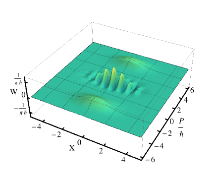
Figure 9: Wigner function for the Schrödinger cat state. Here $\alpha=1/\hslash^{2}$ and $P_{0}=4\hslash$, such that $k=4$.

Using the expression (80) we get:

$$\delta(\Psi)=N^{2}-1+\frac{N^{2}}{\sqrt{2\pi}}\int_{-\infty}^{+\infty}e^{-\frac{z^{2}}{2}}\left|\cos(2kz)\right|dz.$$ (81)

We plot this function in Fig. 10.

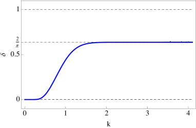
Figure 10: Indicator $\delta(\Psi)$ for the Schrödinger cat state. In the limit $k\rightarrow\infty$ the value $\tfrac{2}{\pi}\approx 0.637$ is approached, while for $k\rightarrow 0$ the state becomes coherent $\delta(\Psi)=0$.

One can show that there exists the following limit:

$$\lim_{k\rightarrow\infty}\delta(\Psi)=\frac{2}{\pi}\approx 0.637.$$ (82)

The regions of the negative values of the Wigner function are specified by the inequality:

$$\cosh(4PP_{0}\alpha)e^{-2P_{0}^{2}\alpha}+\cos\left(\frac{2P_{0}X}{\hslash}\right)<0.$$ (83)

Due to the periodicity of the cosine function we obtain an infinite set of ellipse-like regions of negative values of the Wigner function, as shown in Fig. 11.

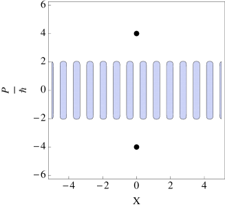
Figure 11: Regions where the Wigner function for the CS cat state assumes its negative values. The black dots represent peaks of the two constituent states.

The area of each such region can be expressed as follows

$$A=\frac{\hslash}{2}\frac{e^{-2k^{2}}}{k^{2}}\int_{1}^{e^{2k^{2}}}\frac{\text{arccosh}(z)}{\sqrt{1-e^{-4k^{2}}z^{2}}}dz\approx\pi\frac{\hslash}{2}=\frac{h}{4}.$$ (84)

The value of above integral was found numerically for a broad range of the parameter $k$, exhibiting independence on the value of $k$. While we were not able to determine the above integral analytically, in the $k\rightarrow 0$ limit, after change of variables, it reduces to

$$\lim_{k\rightarrow 0}A=\hslash\int_{0}^{1}\frac{dz}{\sqrt{1-z^{2}}}=\hslash\frac{\pi}{2}=\frac{h}{4},$$ (85)

in agreement with the numerical result. Thus, while passing to the case of the standard coherent states the area of the negative parts of the Wigner function is preserved. This may seem to be inconsistent since there are no regions of negative values for the coherent states at all. However, this discrepancy is only apparent. In fact, in the limit $k\rightarrow 0$ the domains of $W<0$ elongate in the P direction and disperse in the X direction. In the limit $k\rightarrow 0$, separation between these domains tends to infinity. In short, the domains of $W<0$ escape to infinity in the limit $k\rightarrow 0$, maintaining its areas.

It is interesting to notice that the area (84) is the same as in the case of the $|1\rangle$ Fock state of the harmonic oscillator. This coincidence may exhibit some deeper properties of the formulation of quantum mechanics on phase space schleichbook01 ; zachosetalbook06 .

VII Soliton-like state

VII.1 Construction

In this section we study a state given by superposition of the eigenstates of the Hamiltonian with the profile

$$f(P)\propto\frac{1}{\cosh\left(a(P-P_{0})\right)}.$$ (86)

We will see that while this profile looks qualitatively similar to the Gaussian distribution, its properties are significantly different. In particular, the corresponding Wigner function takes negative values. We have

$$\Psi_{P_{0}}(Q)=\sqrt{\frac{\pi}{4a\hslash}}\frac{e^{\frac{i}{\hslash}P_{0}Q}}{\cosh\left(\frac{\pi}{2a\hslash}Q\right)}.$$ (87)

This state is also of the hyperbolic secant form, since the hyperbolic secant function is a fixed point of the Fourier transform, as the Gaussian distribution.

It is worth mentioning that the obtained state has the form of the so-called bright soliton, which is a solution of the Gross-Pitaevskii equation describing Bose-Einstein condensate. For experimental evidences of such soliton states see for instance beckeretal08 ; Khayk ; Cornish .

The mean values of the canonical variables are

$$\langle\hat{Q}\rangle=T,~{}~{}~{}~{}~{}~{}\langle\hat{P}\rangle=P_{0}.$$ (88)

Therefore the classical constant of integration $c_{1}$ is fixed to be zero, while integration constant $c_{2}=P_{0}$.

The covariance is equal to

$$C_{QP}=0.$$ (89)

The dispersions are

$$\sigma_{Q}=\frac{a\hslash}{\sqrt{3}},$$ (90)

and

$$\sigma_{P}=\frac{1}{a\hslash}\cdot\frac{\pi}{\sqrt{3}}\cdot\frac{\hslash}{2}$$ (91)

Based on the above, the uncertainty relation is satisfied

$$\sigma_{Q}\sigma_{P}=\frac{\pi}{3}\cdot\frac{\hslash}{2}\simeq 1.0472\cdot\frac{\hslash}{2}>\frac{\hslash}{2}\,.$$ (92)

The uncertainty differs only by the factor $\frac{\pi}{3}\approx 1.0472$ from the case of minimal uncertainty realized by the standard coherent states.

VII.2 Wigner function

Inserting the wave function (87) into the definition of the Wigner function we obtain the integral

$$W(X,P)=\frac{1}{a\hslash^{2}}\int_{0}^{\infty}\frac{\cos\left(\frac{2y}{\hslash}(P-P_{0})\right)dy}{\cosh\left(\frac{\pi}{a\hslash}X\right)+\cosh\left(\frac{\pi}{a\hslash}y\right)}.$$ (93)

This integral can be calculated analytically by using the formula (see Integral 3.983 in Ref. Gradshteyn )

$$\int_{0}^{\infty}\frac{\cos(ay)}{b\cosh(\beta y)+c}dy=\frac{\pi\sin\left(\frac{a}{\beta}\text{arccosh}\left(\frac{c}{b}\right)\right)}{\beta\sqrt{c^{2}-b^{2}}\sinh\left(\frac{a\pi}{\beta}\right)},$$ (94)

which holds for $c>b>0$, leading to

$$W(X,P)=\frac{1}{\hslash}\frac{\sin\left(\frac{2(P-P_{0})}{\hslash}X\right)}{\sinh(2(P-P_{0})a)\sinh\left(\frac{\pi}{a\hslash}X\right)}.$$ (95)

We plot this function in Fig. 12.

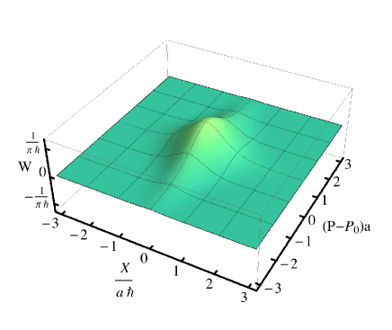
Figure 12: Wigner function for the soliton-like state.

Figure 13: Regions where the Wigner function for the soliton-like state assumes its negative values.

By employing the integral

$$\int_{0}^{\infty}\frac{\sin(\alpha y)}{\sinh(\beta y)}dy=\frac{\pi}{2\beta}\tanh\left(\frac{\alpha\pi}{2\beta}\right)$$ (96)

one can verify that

$$\int_{-\infty}^{+\infty}W(X,P)dP=\frac{\pi}{4a\hslash}\frac{1}{\cosh^{2}\left(\frac{\pi}{2a\hslash}X\right)}$$ (97)

as expected.

VII.3 Superposition of soliton-like states

The normalization function is equal to

$$N=\frac{1}{\sqrt{1+\frac{2P_{0}a}{\sinh(2P_{0}a)}}}.$$ (98)

The interference part of the Wigner function is found to be

$$W_{\text{int}}=\frac{N^{2}}{\hslash}\frac{\cos\left(\frac{2P_{0}}{\hslash}X\right)\sin\left(\frac{2P}{\hslash}X\right)}{\sinh(2Pa)\sinh\left(\frac{\pi}{a\hslash}X\right)}.$$ (99)

Figure 14 presents the Wigner function.

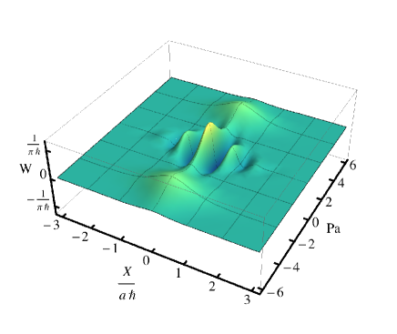
Figure 14: Wigner function for the superposition of soliton-like states for $P_{0}a=4$.

In Fig. 15 we show negative domains of the Wigner function.

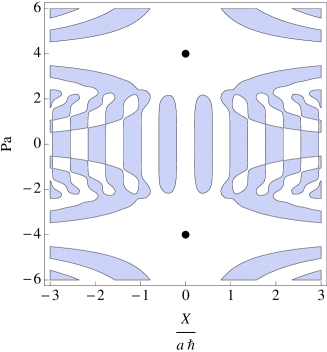
Figure 15: Regions where the Wigner function for the soliton-like cat state assumes its negative values. The black dots represent peaks of the two constituent states.

The areas of the finite domains of $W<0$ are $A\approx 1.00288\cdot\tfrac{h}{4}>\tfrac{h}{4}$.

VIII Decoherence

In quantum mechanics, we are dealing with quantum systems, observers and environments. Because there is always some interaction between quantum system and its environment, quantum systems are never perfectly isolated. Due to this interaction, quantum systems form an entangled state with its environment. The environmental degrees of freedom are however inaccessible to observer. Therefore, from the observer point of view, a quantum system is described by a mixed quantum state, being a statistical mixture of so-called pointer states. These einselected states have properties closest to the classical realm. This process of interaction of the quantum system with its environment, leading to emergence of the classical behavior, is called decoherence Zurek:1991vd ; Zurek:2003zz ; Zurek:1992mv .

In this paper we consider a minisuperspace cosmological model with two-dimensional phase space, parametrized by $Q$ and $P$. It describes dynamics of a global degree of freedom of the universe - the scale factor. At the quantum level, state of this system was described by a pure state in the Hilbert space $\mathcal{H}_{S}=L^{2}(\mathbb{R},dQ)$.

Phase space of the Universe is however much richer and forms the so-called superspace. There is an infinite number of degrees of freedom describing the inhomogeneities of the gravitational and matter fields. These degrees of freedom (irrelevant degrees of freedom) can serve as an environment for our system (relevant degrees of freedom). It was tacitly assumed here that the inhomogeneities have no influence on the background dynamics. However, this assumption can be violated at some stages of the cosmic evolution.

The state of our system and its environment is described by a vector in the Hilbert space which is the tensor product $\mathcal{H}_{S}\otimes\mathcal{H}_{E}$, where $\mathcal{H}_{E}$ is the Hilbert space of the environment states. It is worth noticing here that the total state describing the system plus environment is pure, since there is no environment with respect to the Universe. However, from the perspective of an internal observer, the state of the quantum system, immersed in the inaccessible environment, is mixed.

Let us consider a possible situation, which can arise in the cosmological context. Namely let us assume that the state of our minisuperspace model is described by the Schrödinger cat state composed of two coherent states, as was studied in Sec. VI. Due to interaction with environment, this state forms an entangled state with its environment. This state is described by the total density matrix $\hat{\rho}_{E+S}$. However, for an observer, only elements of the reduced density matrix $\hat{\rho}_{S}=\text{tr}_{E}(\hat{\rho}_{E+S})$ are available, which forms a statistical mixture of two coherent states

$$\hat{\rho}_{E}=\frac{1}{2}|P_{0}\rangle\langle P_{0}|+\frac{1}{2}|-P_{0}\rangle\langle-P_{0}|.$$ (100)

Therefore, while the initial pure state contained interference terms in its density matrix

$$\hat{\rho}=|\Psi\rangle\langle\Psi|,$$ (101)

they were suppressed by interaction with the environment.

The described process of decoherence can be clearly seen at the level of the Wigner functions. Namely, in this process the interference part of the Wigner function is suppressed leading to the statistical mixture of two coherent states.

Employing the general definition of the Wigner function, which applies also to mixed states:

$$W(X,P)=\frac{1}{\pi\hslash}\int_{-\infty}^{+\infty}\langle X-y|\hat{\rho}|X+y\rangle e^{2iPy/\hslash}dy,$$ (102)

we get

$$W(X,P)=\frac{1}{2}(W_{+}+W_{-}),$$ (103)

for the reduced density matrix (100). We show this function in Fig. 16.

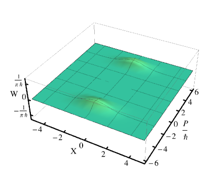
Figure 16: Wigner function for the decohered Schrödinger cat state.

By comparing Fig. 16 with Fig. 9, it is clear that during the decoherence process the interference pattern disappears, and the state of the universe reduces to the statistical mixture of the two uncorrelated universes.

We suggest two possible interpretations of the observed emergence of two separated universes:

• The two signs of the $P$ variable may be related with the two possible orientations of triad. Therefore, the Schrödinger cat state may describe universe being in superposition of two orientations of the triad. These orientations correspond to the two values $\pm P_{0}$. Due to the interaction with environment, the state of the universe breaks into a statistical mixture of the two universes with positive and negative orientations, respectively. Such possibility was recently studied in Ref. Kiefer:2012kp . It was shown that fermionic matter serves as a natural environment with respect to which decoherence of the triad orientation may occur.

• According to the BKL scenario BKL22 ; BKL33 , the space-points decouple while approaching the cosmic singularity. Such a behavior, known also as the asymptotic silence, appears already at the classical level, but is also predicted within some approaches to quantum gravity. In particular, recent investigations of the perturbative sector of LQC exhibited occurrence of the asymptotic silence due to the discrete nature of space at the Planck scale Mielczarek:2012tn .

  In the state of asymptotic silence, each small neighbourhood of a point of space can be described by a homogenous model. In particular, in the BKL scenario, each such small homogeneous ‘universe’ is described by the Kasner solution. Turning on some nonvanishing coupling between the different space points leads to transitions between Kasner phases for each of those small universes.

  In the idealized situation, each of the space points may be described by the homogeneous and isotropic model as the one considered in this paper. The Schrödinger cat state describes the simplest superposition of two such small universes with opposite values of $P_{0}$ respectively.

IX Entropies

Due to the possible relation to the flow of time, it is tempting to introduce the notion of entropy in quantum cosmology. In particular, in our earlier paper Mielczarek:2012qs , the following definition of entropy of squeezing was proposed:

$$S:=k_{B}\ln\left(\frac{\sigma_{Q}\sigma_{P}\sqrt{1-\rho^{2}}}{\hslash/2}\right),$$ (104)

where $\rho=C_{QP}/(\sigma_{Q}\sigma_{P})\in[-1,1]$ is a dimensionless correlation coefficient, measuring phase squeezing of a quantum state. This entropy is defined such that it is equal to zero for the states saturating the Schrödinger-Robertosn uncertainty relation and is positive definite for other pure states.

It was shown that while considering dynamics of a standard coherent state (Gaussian state) in the $\mathcal{H}_{1}$ Hilbert space, qualitative behavior of (104) agrees with predictions based on the von Neumann entropy of mixed states:

$$S_{N}=-k_{B}\text{tr}[\hat{\rho}\ln\hat{\rho}].$$ (105)

In particular, the entropy (104) assumes its minimal value at the bounce, when the energy density reaches its maximal value Mielczarek:2012qs .

The density matrix is invariant under unitary transformation, $\hat{\rho}\rightarrow\hat{U}\hat{\rho}\hat{U}^{\dagger}$, which amounts to unitary invariance of the von Neumann entropy. This reflects the fact that, at the classical level, Gibbs entropy as well as Boltzmann entropy are invariant under canonical transformations.

The entropy (104) is however not invariant with respect to the canonical transformations. For the variables $(q,p)$ and $(Q,P)$ related by the canonical transformation, the entropy can take a completely different form. In particular, while in one coordinate system it is time dependent function, in another one it takes a constant value in time. Such a situation happens e.g. in the case of standard coherent states considered in this paper. In Ref. Mielczarek:2012qs we have studied the evolution of dispersions $\sigma_{q}$, $\sigma_{p}$ and $C_{qp}$ for such a state. All of these variables exhibited time dependence and both amplitude and phase squeezing in time were observed.

However, as shown in Sec. VI the values of $\sigma_{Q}$, $\sigma_{P}$ and $C_{QP}$ are constant in time. Moreover, also for the other states in this paper, time independence of dispersions and covariance was observed. This turns out to be a general property, resulting from the particular form of the Hamiltonian $H=P$. For such a system, the time evolution manifests as a shift of the Q variable, $Q\rightarrow Q-T$. Therefore, the whole dynamics reduces to translations of the Wigner function with preservation of its shape. Such translation does not affect the initial spreads and covariance, as well as the higher moments. This behavior, is precisely the same as observed for the photon wave-packets, for which dispersions are preserved in time due to linear dispersion relation.

Due to the above property, the Wehrl entropy wehrl , which employs the Husimi husimi function, is also expected to take constant values for the state considered in this paper. However, it is worth stressing that the von Neumann’s entropy grows during decoherence of the Schrödinger cat state studied in the previous section. This increase of the von Neumann entropy exhibits the fact that the part of information about the system is hidden in the environment. Such an increase of entropy can contribute to the total increase of the entropy of the universe and the observed arrow of time.

X Relation to observations

Each of the states considered in this paper aims to describe global degrees of freedom of the universe in the quantum epoch. There is no theoretical principle which could be used to distinguish one of these states in the context of quantum cosmology. Such a goal can be achieved only by confronting theoretical predictions with observational data. The task is however extremely difficult due to the lack of well established probes of the Planck epoch. Nevertheless, a significant progress in this direction has been made in recent years. Especially, by employing scalar and tensor perturbations which can be produced during the quantum epoch. They may lead to some imprints on the spectrum of the cosmic microwave background (CMB) radiation. In particular, by using observations of the CMB one can determine the value of the Hubble factor

$$\mathcal{H}:=\frac{1}{a}\frac{da}{dt},$$ (106)

during the phase of inflation, which follows the quantum epoch. This measurement can be used to put constraints on the quantum fluctuations of the Hubble factor in a given state describing the Universe. Namely, we expect that relative quantum fluctuations of the Hubble parameter are smaller than the relative uncertainty of the measurement. It means that:

$$\frac{\sigma_{\mathcal{H}}}{\langle\hat{\mathcal{H}}\rangle}<\frac{\Delta\mathcal{H}}{\mathcal{H}},$$ (107)

where $\mathcal{H}$ is the measured value of the Hubble parameter and $\Delta\mathcal{H}$ is the uncertainty of the measurement. As shown in Ref. Mielczarek:2012qs , based on the seven years observations of the WMAP satellite, uncertainty of the measurement of the Hubble at some fixed point of inflation is $\frac{\Delta\mathcal{H}}{\mathcal{H}}\approx 0.19$. Whereas, measurements of the present value of the Hubble factor give us $\frac{\Delta\mathcal{H}}{\mathcal{H}}\approx 0.02$. Both results are in agreement with our expectation that relative quantum fluctuations should satisfy

$$\frac{\sigma_{\mathcal{H}}}{\langle\hat{\mathcal{H}}\rangle}\ll 1.$$ (108)

Such a restriction is usually considered as a condition of semi-classicality Corichi:2007am .

One can also interpret the above as a requirement of the correspondence principle. Namely, in the limit of large quantum numbers the quantum mechanics should reproduce classical dynamics. Here, the limit of the large quantum numbers corresponds to the limit of large volume.

Based on the above we can guess, as confirmed by the astronomical observations, that the relative fluctuations of the Hubble parameter may be used to indicate semi-classicality of the expanding universe. In what follows we use this restriction to put constraints on the parameters of considered states of the universe.

The important observation is that in the limit of large volumes $(|p|\rightarrow\infty,q\rightarrow 0)$, the value of the parameter $q$ is proportional to the Hubble factor: $q=\gamma\lambda\mathcal{H}$. But this is precisely where our observational constraints can be applied. Therefore, in the considered limit, the constraint (107) leads to

$$\frac{\sigma_{q}}{\langle\hat{q}\rangle}<\frac{\Delta\mathcal{H}}{\mathcal{H}}.$$ (109)

The task is now to determine the left hand side of the above equation for the examined states in the limit $q\rightarrow 0$. Since we investigated properties of the states in the Hilbert space $\mathcal{H}_{2}$, we have to express the parameter $q$ in terms of $Q$. Employing the definition (10), we can write

$$q=2\text{arctan}\left(e^{X+T}\right)=\epsilon e^{X}+\mathcal{O}(\epsilon^{3}),$$ (110)

where we have performed expansion in the parameter $\epsilon=e^{T}$, which tends to zero in the limit $T\rightarrow-\infty$. In this limit $q\rightarrow 0$.

Now we express the first and the second moment of the variable $q$ as follows:

$$\langle\hat{q}\rangle = 2\epsilon\int_{-\infty}^{+\infty}e^{X}|\Psi(X)|^{2}dX+\mathcal{O}(\epsilon^{3}),$$ (111)

$$\langle\hat{q}^{2}\rangle = 4\epsilon^{2}\int_{-\infty}^{+\infty}e^{2X}|\Psi(X)|^{2}dX+\mathcal{O}(\epsilon^{4}).$$ (112)

Using the above expressions, the relative uncertainty of $q$ in the limit $\epsilon\rightarrow 0$ can be written as

$$\lim_{\epsilon\rightarrow 0}\frac{\sigma_{q}}{\langle\hat{q}\rangle} = \lim_{\epsilon\rightarrow 0}\sqrt{\frac{\langle\hat{q}^{2}\rangle}{\langle\hat{q}\rangle^{2}}-1}$$ (113)

$$= \sqrt{\frac{\int_{-\infty}^{+\infty}e^{2X}|\Psi(X)|^{2}dX}{\left(\int_{-\infty}^{+\infty}e^{X}|\Psi(X)|^{2}dX\right)^{2}}-1}.$$

The condition of semi-classicality (108) now states that:

$$\lim_{\epsilon\rightarrow 0}\frac{\sigma_{q}}{\langle\hat{q}\rangle}\ll 1.$$ (114)

In what follows, we will use this restriction to put constraints on the parameters of our models.

X.1 Boxcar state

For the boxcar state, the following integrals can be easily found:

$$\int_{-\infty}^{+\infty}e^{X}|\Psi(X)|^{2}dX = \frac{2}{L}\sinh\left(\frac{L}{2}\right),$$ (115)

$$\int_{-\infty}^{+\infty}e^{2X}|\Psi(X)|^{2}dX = \frac{1}{L}\sinh(L).$$ (116)

By applying those integrals to expression (113), we obtain

$$\lim_{\epsilon\rightarrow 0}\frac{\sigma_{q}}{\langle\hat{q}\rangle}=\sqrt{\frac{L/2}{\tanh(L/2)}-1}.$$ (117)

Employing the condition of semi-classicality (114) we obtain the following transcendental ineqality

$$2\tanh(L/2)\gg L/2.$$ (118)

This equation can be solved numerically leading to the restriction

$$L\ll 3.83.$$ (119)

Only for such values the state reveals the correct semi-classical limit. As we see, by imposing the requirement of an agreement with the semi-classical behavior of the universe in the expanding branch, a dominant part of the range of the parameter $L$ is excluded.

X.2 Schrödinger cat composed of boxcar states

For the Schrödinger cat composed of boxcar states, the formula (113) can be expressed as follows

$$\lim_{\epsilon\rightarrow 0}\frac{\sigma_{q}}{\langle\hat{q}\rangle}=\sqrt{\frac{e^{L}(1+4\tilde{P}_{0}^{2})^{2}(L\tilde{P}_{0}+\sin(L\tilde{P}_{0}))(\tilde{P}_{0}\cosh(L)\sin(L\tilde{P}_{0})+(1+\tilde{P}_{0}^{2}+\cos(L\tilde{P}_{0}))\sinh(L))}{((\tilde{P}_{0}+\tilde{P}_{0}^{3})((-1+e^{L})(1+4\tilde{P}_{0}^{2})+(-1+e^{L})\cos(L\tilde{P}_{0})+2(1+e^{L})\tilde{P}_{0}\sin(L\tilde{P}_{0}))^{2})}-1},$$ (120)

where $\tilde{P_{0}}=P_{0}/\hslash$. This equation simplifies to (117), in the limit $\tilde{P_{0}}\rightarrow 0$. Based on equation (120), in Fig. 17 we show the region of the parameter space for which $\lim_{\epsilon\rightarrow 0}\frac{\sigma_{q}}{\langle\hat{q}\rangle}<1$. In this region, relative quantum fluctuations of the Hubble factor in the large volume limit are smaller than unity.

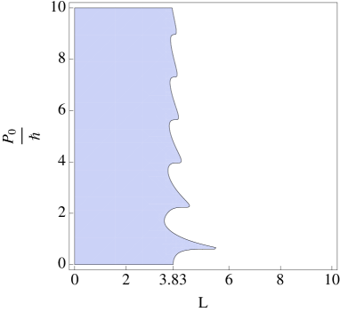
Figure 17: Shadowed region of the parameter space represents $\lim_{\epsilon\rightarrow 0}\frac{\sigma_{q}}{\langle\hat{q}\rangle}<1$, a necessary condition for semi-classicality, which holds in a neighborhood of the origin.

Therefore, only for the values of the parameters belonging to this region, the Schrödinger cat composed of boxcar states has a semiclassical limit. It is worth noticing that for $P_{0}/\hslash=0$, the obtained constraints overlap with (119), as expected.

X.3 Standard coherent state

For the standard coherent state

$$\int_{-\infty}^{+\infty}e^{X}|\Psi(X)|^{2}dX = \exp\left[\frac{(2\Re a_{2}+1)^{2}}{8\Re a_{1}}\right],$$ (121)

$$\int_{-\infty}^{+\infty}e^{2X}|\Psi(X)|^{2}dX = \exp\left[\frac{(2\Re a_{2}+2)^{2}}{8\Re a_{1}}\right].$$ (122)

Using these integrals we get

$$\lim_{\epsilon\rightarrow 0}\frac{\sigma_{q}}{\langle\hat{q}\rangle}=\sqrt{\exp\left[\frac{1-2(\Re a_{2})^{2}}{4\Re a_{1}}\right]-1}.$$ (123)

The condition of reality of the above expression together with the requirement of semi-classicality can be written as

$$0\leq\frac{1-2(\Re a_{2})^{2}}{4\Re a_{1}}\ll\ln 2.$$ (124)

Because $\Re a_{1}>0$, the two conditions must hold:

$$(\Re a_{2})^{2} \leq\frac{1}{2},$$ (125)

$$\Re a_{1} \gg\frac{1-2(\Re a_{2})^{2}}{4\ln 2}.$$ (126)

For the special case $\Re a_{2}=0$ $(\alpha=0)$ we obtain

$$\Re a_{1}\gg\frac{1}{4\ln 2},$$ (127)

which yields the following constraint on dispersion

$$\sigma_{Q}\ll\sqrt{\ln 2}\approx 0.83.$$ (128)

X.4 Schrödinger cat composed of standard coherent states

For the Schrödinger’s cat state we have

$$\int_{-\infty}^{+\infty}e^{X}|\Psi(X)|^{2}dX=$$

$$=N^{2}e^{\frac{\hslash^{2}\alpha}{2}}\left[1+e^{-2P_{0}^{2}\alpha}\cos(P_{0}\alpha\hslash)\right],$$ (129)

$$\int_{-\infty}^{+\infty}e^{2X}|\Psi(X)|^{2}dX=$$

$$=N^{2}e^{2\hslash^{2}\alpha}\left[1+e^{-2P_{0}^{2}\alpha}\cos(4P_{0}\alpha\hslash)\right].$$

Based on the above we find

$$\lim_{\epsilon\rightarrow 0}\frac{\sigma_{q}}{\langle\hat{q}\rangle}=\sqrt{\frac{e^{\hslash^{2}\alpha}}{N^{2}}\frac{\left[1+e^{-2P_{0}^{2}\alpha}\cos(4P_{0}\alpha\hslash)\right]}{\left[1+e^{-2P_{0}^{2}\alpha}\cos(P_{0}\alpha\hslash)\right]^{2}}-1}.$$ (130)

In the limit $P_{0}\rightarrow 0$, this equation simplifies to

$$\lim_{\epsilon\rightarrow 0}\frac{\sigma_{q}}{\langle\hat{q}\rangle}=\sqrt{e^{\alpha\hslash^{2}}-1}.$$ (131)

The semi-classicality condition (114) applied to (130) leads to the following constraint

$$\frac{e^{\hslash^{2}\alpha}}{N^{2}}\frac{\left[1+e^{-2P_{0}^{2}\alpha}\cos(4P_{0}\alpha\hslash)\right]}{\left[1+e^{-2P_{0}^{2}\alpha}\cos(P_{0}\alpha\hslash)\right]^{2}}\ll 2.$$ (132)

In Fig. 18 we show the region of the parameter space for which $\lim_{\epsilon\rightarrow 0}\frac{\sigma_{q}}{\langle\hat{q}\rangle}<1$, indicating the part of the parameter space within which the semi-classicality condition is fulfilled.

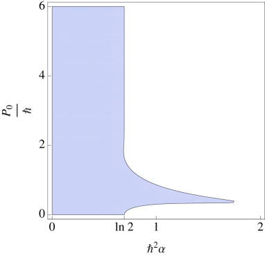
Figure 18: For the state to be semiclassical the parameters must lie within the shadowed region. Semi-classicality holds in a neighborhood of the origin.

In the special case when $P_{0}\rightarrow 0$ (two peaks overlap) the condition (132) simplifies to

$$\hslash^{2}\alpha\ll\ln 2\approx 0.693.$$ (133)

By using (73), the above constrain leads to

$$\sigma_{Q}\ll\sqrt{\ln 2}\approx 0.83,$$ (134)

which, as expected, is in agreement with the case of the standard coherent state for $\Re a_{2}=0$.

X.5 Soliton-like state

For the soliton-like state, the following integrals can be determined:

$$\int_{-\infty}^{+\infty}e^{X}|\Psi(X)|^{2}dX = \frac{a\hbar}{\sin(a\hbar)},$$ (135)

$$\int_{-\infty}^{+\infty}e^{2X}|\Psi(X)|^{2}dX = \frac{2a\hbar}{\sin(2a\hbar)},$$ (136)

for $a\hbar<\pi$ in the first case and $a\hbar<\frac{\pi}{2}$ in the second case. The integrals are not convergent above these ranges.

By applying the above integrals to expression (113), we obtain

$$\lim_{\epsilon\rightarrow 0}\frac{\sigma_{q}}{\langle\hat{q}\rangle}=\sqrt{\frac{\tan(a\hslash)}{a\hslash}-1}$$ (137)

Employing the condition of semi-classicality (114) we obtain

$$\tan(a\hslash)\ll 2a\hslash,$$ (138)

which can be solved numerically leading to

$$a\hslash\ll 1.17.$$ (139)

X.6 Schrödinger cat composed of soliton-like states

For the Schrödinger cat composed of soliton-like states on can also find analytical formula for $\lim_{\epsilon\rightarrow 0}\frac{\sigma_{q}}{\langle\hat{q}\rangle}$. However, because the obtained formula is quite long, we present, in Fig. 19, only the the resulting constraint $\lim_{\epsilon\rightarrow 0}\frac{\sigma_{q}}{\langle\hat{q}\rangle}<1$.

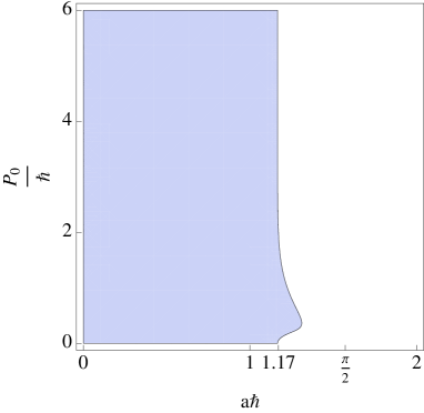
Figure 19: For the state be semiclassical the parameters must lie within the shadowed region. Semi-classicality holds in a neighborhood of the origin.

As expected, for $P_{0}=0$ the constraint (139) is recovered.

XI Conclusions

In this paper we have studied dynamics of the quantum bouncing universe for a variety of quantum states. We examined properties of the following states: boxcar state, standard coherent state, and soliton-like state, as well as Schrödinger’s cat states constructed from each of them respectively. Characteristics of these states such as quantum moments and Wigner functions were investigated.

We have found a canonical transformation $\Gamma_{1}\ni(q,p)\rightarrow(Q,P)\in\Gamma_{2}$, which transforms initial non-polynomial Hamiltonian $H_{1}=p\sin q$ into a simple linear Hamiltonian $H_{2}=P$, which resembles the Hamiltonian of a photon. The unitary map $\mathcal{U}:\mathcal{H}_{1}\rightarrow\mathcal{H}_{2}$, corresponding to the canonical transformation was also constructed.

Analysis of the Wigner functions for considered states enabled us to relate quantum dynamics with the classical phase space structure. It was shown that, the boxcar state, standard coherent state, and soliton-like state can reproduce all trajectories on the phase space. However, Schödinger cat states, which are less classical than the above states, can follow only the trajectories with $P=0$, since $\langle\hat{P}\rangle=0$ for these states. By analyzing the classical limit (large volumes) we have found that all considered states have proper semi-classical behavior for some values of parameters. We have determined ranges of the parameters. The obtained semi-classical states are complementary to those found in Refs. Corichi:2011rt ; Corichi:2011sd .

Furthermore, analysis of the Wigner functions for the considered states leads to the two general observations:

• For the investigated states we have found that $W\left(\langle X\rangle,\langle P\rangle\right)=1/\hslash\pi.$ This may suggest that such relation is fulfilled for some broad class of pure states. For mixed states this relation does not hold as can be seen for the decohered Schrödinger cat state.

• We have found that the minimal area of the domain of the negative values of the Wigner function may be bounded from below by the factor $h/4$ for some class of states. In other words, we conjecture that $\oint PdQ\geq h/4$, for a region of the negative values of the Wigner function. The approximate value $h/4$ was found numerically for the Schrödinger cat states composed of two standard coherent states as well as for the Schrödinger cat state composed of two soliton-like states. For the peculiar case of the Schrödinger cat of two boxcar states the above inequality is not fulfilled, which may result from the fact that the uncertainty relation is not well defined for this state. Therefore, it is possible that the relation $\oint PdQ\geq h/4$ is valid only if the Schrödinger-Robertson uncertainty relation is satisfied.

Wigner’s function can be reconstructed experimentally by applying methods of quantum tomography. It is interesting to ask if such a method could be applied also in the cosmological realm? The answer to this question is however closely related to the meaning of reduction of state in quantum cosmology. In laboratory, in order to determine the shape of the Wigner distribution, an ensemble of systems prepared in the same quantum state is necessary. Then, by collecting measurements performed on each system, the structure of the phase space distribution can be recovered by virtue of the inverse Radon transform. Possibility of such a reconstruction in cosmology is however uncertain due to an absence of a sound notion of quantum measurement for the universe. The problem is due to the fact that there is only one Universe. Therefore, one cannot perform measurements on ensemble of identical universes. However, measurements of expansion rate at different locations (subsystems) can be done. The average expansion at different places is described by the same equation, with similar initial conditions. In such a case, statistical interpretation of quantum mechanics could be applied, and extraction of the Wigner function by quantum tomography would be, in principle, possible. This issue deserves further investigations.

We have also shown that the notion of an entropy of squeezing, introduced in our earlier paper Mielczarek:2012qs is not invariant under canonical transformations. Therefore, it cannot be used as a reliable intrinsic time parameter. The same applies to quantum covariance, which only for some specific coordinates evolves monotonically.

In this paper, we have studied decoherence of the Schrödinger cat state of the minisuperspace model, due to the interaction with the environment. Such a decoherence is a toy model of what could in fact happen in the very early universe. Firstly, this process may describe decoherence of the triad orientation, as already suggested in Ref. Kiefer:2012kp . This is a quite attractive interpretation, since there are two equivalent triad orientations allowed, and the process of decoherence affords an explanation to the emergence of them in the classical world.

Secondly, the Schrödinger cat state can describe superposition of two separated space points in the quantum counterpart of the state of asymptotic silence (quantum BKL scenario). One can speculate that, is such a phase, entire Universe was in highly entangled state. Due to the the decoherence process, the classical BKL scenario, characterized by existence of almost independent homogeneous regions of space, emerged.

In the context of the decoherence, one can speculate what follows: During the quantum phase the entire Universe was in a highly entangled state with small quantum inhomogeneities described by hypothetical quantum BKL scenario. Due to expansion, the evolution entered classical BKL scenario characterized by the existence of almost independent homogeneous but anisotropic regions of space. Later, each of these regions turned into an isotropic region that could be modeled by the FRW type spacetime. Due to entanglement during the quantum phase, all space regions became correlated. Such quantum correlation may explain observed causal connection of the cosmic microwave background (CMB) radiation without need of inflation.

- (1) A. Ashtekar and P. Singh, “Loop Quantum Cosmology: A Status Report,” Class. Quant. Grav. 28 (2011) 213001 [arXiv:1108.0893 [gr-qc]].
- (2) M. Bojowald, “Loop quantum cosmology”, Living Rev. Rel. 8 (2005) 11.
- (3) P. Dzierzak, P. Malkiewicz and W. Piechocki, “Turning big bang into big bounce. 1. Classical dynamics”, Phys. Rev. D 80 (2009) 104001 [arXiv:0907.3436 [gr-qc]].
- (4) P. Malkiewicz and W. Piechocki, “Turning big bang into big bounce: II. Quantum dynamics”, Class. Quant. Grav. 27 (2010) 225018 [arXiv:0908.4029 [gr-qc].
- (5) J. Mielczarek and W. Piechocki, “Evolution in bouncing quantum cosmology”, Class. Quant. Grav. 29 (2012) 065022 [arXiv:1107.4686 [gr-qc]].
- (6) J. Mielczarek and W. Piechocki, “Gaussian state for the bouncing quantum cosmology”, Phys. Rev. D 86 (2012) 083508 [arXiv:1108.0005 [gr-qc]].
- (7) K. A. Meissner, “Black hole entropy in loop quantum gravity,” Class. Quant. Grav. 21 (2004) 5245 [gr-qc/0407052].
- (8) M. Bojowald, “What happened before the Big Bang?”, Nature Phys. 3N8 (2007) 523.
- (9) Authors are grateful to Antonia Zipfel for pointing out the possibility of such a behavior.
- (10) A. Perelomov, Generalized coherent states and their applications, (Berlin: Springer, 1986).
- (11) J.-P. Gazeau, Coherent States in Quantum Physics (Berlin: Wiley-VCH, 2009).
- (12) J. S. Walker, A Primer on Wavelets and Their Scientific Applications, Sd Edition (Studies in Advanced Mathematics), (Chapman and Hall/CRC, 2008).
- (13) A. Ourjoumtsev, H. Jeong, Rosa Tualle-Brouri and P. Grangier, “Generation of optical ‘Schrödinger cats’ from photon number states”, Nature 448 (2007) 784.
- (14) C. Kiefer and C. Schell, “Interpretation of the triad orientations in loop quantum cosmology”, arXiv:1210.0418 [gr-qc].
- (15) A. Kenfeck and K. Życzkowski, “Negativity of the Wigner function as an indicator of nonclassicality”, J. Opt. B: Quantum Semiclass. Opt. 6 (2004) 396.
- (16) R. L. Hudson, “When is the Wigner quasi-probability density non-negative?,” Rep. Math. Phys. 6 (1974) 249.
- (17) T. Brocker and R. F. Werner, “Mixed states with positive Wigner functions,” J. Math. Phys. 36 (1995) 62.
- (18) W. P. Schleich, Quantum Optics in Phase Space (Berlin: Wiley-VCH, 2001).
- (19) C. K. Zachos, D. B. Fairlie, and T. L. Curtright (eds) Quantum Mechanics In Phase Space, World Scientific Series in 20th Century Physics 34 (World Scientific 2006).
- (20) C. Becker et al “Oscillations and interactions of dark and dark-bright solitons in Bose-Einstein condensates”, Nature Physics 4 (2008) 496501.
- (21) L. Khaykovich et al. “Formation of a Matter-Wave Bright Soliton”, Science 296 (2002) 1290.
- (22) S. L. Cornish, S. T. Thompson, and C. E. Wieman, “Formation of Bright Matter-Wave Solitons during the Collapse of Attractive Bose-Einstein Condensates”, Phys. Rev. Lett. 96 (2006) 170401.
- (23) I. S. Gradshteyn and I. M. Ryzhik, Table of Integrals, Series, and Products (Alan Jeffrey, 1994), Fifth edition.
- (24) W. H. Zurek, “Decoherence and the transition from quantum to classical”, Phys. Today 44N10 (1991) 36.
- (25) W. H. Zurek, “Decoherence, einselection, and the quantum origins of the classical”, Rev. Mod. Phys. 75 (2003) 715.
- (26) W. H. Zurek, S. Habib and J. P. Paz, “Coherent states via decoherence”, Phys. Rev. Lett. 70 (1993) 1187.
- (27) V. A. Belinskii, I. M. Khalatnikov and E. M. Lifshitz, “Oscillatory approach to a singular point in the relativistic cosmology”, Adv. Phys. 19 (1970) 525.
- (28) V. A. Belinskii, I. M. Khalatnikov and E. M. Lifshitz, “A general solution of the Einstein equations with a time singularity”, Adv. Phys. 31 (1982) 639.
- (29) J. Mielczarek, “Asymptotic silence in loop quantum cosmology,” AIP Conf. Proc. 1514 (2012) 81 [arXiv:1212.3527 [gr-qc]].
- (30) A. Wehrl, “General properties of entropy”, Rev. Mod. Phys. 50 (1978) 221.
- (31) K. Husimi, “Some Formal Properties of the Density Matrix”, Proc. Phys. Math. Soc. Jpn. 22 (1940) 264 314.
- (32) A. Corichi and P. Singh, “Quantum bounce and cosmic recall,” Phys. Rev. Lett. 100 (2008) 161302 [arXiv:0710.4543 [gr-qc]].
- (33) A. Corichi and E. Montoya, “Coherent semiclassical states for loop quantum cosmology,” Phys. Rev. D 84 (2011) 044021 [arXiv:1105.5081 [gr-qc]].
- (34) A. Corichi and E. Montoya, “On the Semiclassical Limit of Loop Quantum Cosmology,” Int. J. Mod. Phys. D 21 (2012) 1250076 [arXiv:1105.2804 [gr-qc]].