Two cases of squares evolving by anisotropic diffusion

Abstract

We are interested in an anisotropic singular diffusion equation in the plane and in its regularization. We establish existence, uniqueness and basic regularity of solutions to both equations. We construct explicit solutions showing the creation of facets, i.e. flat regions of solutions. By using the formula for solutions, we rigorously prove that both equations create ruled surfaces out of convex initial conditions as well as do not admit point (local) extrema. We present numerical experiments suggesting that the two flows seem not differ much. Possible applications to image reconstruction is pointed out, too.

1 Introduction

We study two examples of singular diffusion equations. One of them is an anisotropic total variation (TV) flow, the other one is the same equation with the additive isotropic linear diffusion,

$$\frac{\partial u}{\partial t}=\beta\,\text{div}\left(\frac{u_{x_{1}}}{|{u_{x_{1}}}|},\frac{u_{x_{2}}}{|{u_{x_{2}}}|}\right),$$ (1.1)

$$\frac{\partial u}{\partial t}=\gamma\Delta u+\beta\,\text{div}\left(\frac{u_{x_{1}}}{|{u_{x_{1}}}|},\frac{u_{x_{1}}}{|{u_{x_{1}}}|}\right).$$ (1.2)

These problems are considered on a domain in $\mathbb{R}^{2}$. Our goal is to study features of solutions like facets, i.e. flat parts of solutions with normals corresponding to the singular directions. Our study was inspired by the phase transition theory appearing in crystal growth problems and image restoration, where presence of walls and edges plays a significant role, [13], [23], [24].

Let us describe ideas behind this note. The key element of the systems we study is the anisotropy. In both cases this determines the features of solutions. We will see that numerical experiments appear to give almost the same despite fact that the second equation is not degenerate. The most spectacular phenomenon which is observed for this type of problems are flat parts of solutions, connected with very strong diffusion, where $\nabla u=0$. Such effects have been well studied for the isotropic total variation flow. We note that the interest in the TV flow arose from its application to image analysis and reconstruction, [25], [5], [2]. Namely, any regular level sets of solutions to this flow evolve by the mean curvature. This property is used to smooth out contours and in deblurring. We stress that numerical algorithms exploit properties of this flow even implicitly.

The case of anisotropic diffusion is not so well studied. Despite the available papers like [18], [3], the mathematical theory is still far from the excellence. This changes however, because of the interest in algorithms detecting or retaining special image features like edges and corners. A conspicuous example is the paper [10] on 2D bar codes. We observe a growing body of literature devoted to this subject, [22], [7], [14], [16], [15]. We see the need to study evolution equations which are likely to preserve pronounced features of solution or its graphs besides facets, e.g. edges or corners. It turns out that the equations we study here may serve this purpose. The rigorous goals will be stated below, but we also present numerical simulations in section 5, which illustrate the qualitative features of solutions.

We set the following main goals of this paper:

$\clubsuit$  to study facets, the flat parts of solutions, defined by $\nabla u=0$;

$\clubsuit$   to exhibit ruled surfaces, arising when one of the components of the gradient of solution $u$ vanishes;

$\clubsuit$  to construct special solutions, given by the explicit formulas which shows characteristic features of solutions;

$\clubsuit$  to present numerical experiments and to show evolution of interesting model shapes, which were the motivation for looking for analytical results;

$\clubsuit$  to propose a possible application to image processing.

It is surprising that facets and ruled surfaces are the attributes of solutions to both systems. The lack of degeneration in the second model results only in smoothing out effect appearing near ‘corners’ and some dispersion. Hence in practice, one could find the second equation as more suitable for practical applications. Here, we present a series of solutions to both systems, represented by the gray scale. It shows some interesting differences, which nonetheless are very subtle. The initial data are represented by the last picture on Fig. 2.

        

        

Figure 1: Snapshots of evolution by (1.1) (first row) and (1.2) (second row) of the same initial datum

Applications to the phase transition theory are of particular interest, [24], however, systems (1.1) and (1.2) are rather a simplification of more complex models. In the image processing, usefulness may be more straightforward to see. The pictures presented in Section 5 show a possibility of reconstructing images. The diffusion in the second system helps us to restore the picture. Positivity of $\gamma$ gives averaging effects, but strong anisotropic nonlinearity keeps edges in the chosen directions.

The upshot of these experiments is the following. The regularization of a very singular system yields not only smooth solutions but also it preserves the main features of the original equation. We should keep in mind this important observation in our future studies of systems with very singular nonlinear operators.

At this point we note that the system with the added isotropic diffusion behaves like phase field models with respect to free boundary problems including the mean curvature flow. We mention just a few papers exploring the link, [1], [4], [6].

Here, we do not plan to present a consistent theory, but rather to pinpoint a few interesting results and phenomena to find motivation for our future deeper mathematical analysis. In fact, this note can be viewed as an attempt to extend results for one-dimensional systems [17, 20, 21, 19] on the two-dimensional case. To be more precise, we establish existence of solutions to both equations (1.1) and (1.2) by using the theory of nonlinear semigroups. For this purpose we exploit the gradient structure of (1.1) and (1.2). Uniqueness is automatically guaranteed. This is presented in the next section. There we also present exact formulas for solutions. The advantage is that they provide insight into the facet formation problem. Since the formulas do not always fit the framework of semigroup solutions, we recall the notion of a weak solution. The explicit solutions suggest that the flows of (1.1) and (1.2) make ruled surfaces out of the initial data, provided additional conditions are satisfied. This is rigorously established in Section 4. This considerations require quite precise regularity estimates established in Theorem in Section 3.

The paper is organized as follows. In Section 2 we state basic existence results for systems (1.1) and (1.2) coming from the general theory. We point also to a few interesting explicit solutions illustrating typical shapes. In Section 3 we show that the solutions are of better regularity, provided the initial data are smooth enough. Next we prove conditional results, which explain why flat regions and ruled surfaces are typical for graphs of solutions. In Section 5 we concentrate on numerical analysis and obtain a few interesting numerical solutions. These results show more direct phenomena which are able to be captured by the systems. In the appendix we present more complex example of an explicit solutions to (1.1).

2 Existence

We will use general tools exploiting the structure of the problem. In order to use the semigroup theory we notice that we present equations (1.1), (1.2) as gradient flows of corresponding functionals on $L^{2}(\Omega)$. We set

$$\Phi_{0}(u)=\left\{\begin{array}[]{ll}\int_{\Omega}\beta(|u_{x_{1}}|+|u_{x_{2}}|)&\hbox{if }u\in BV(\Omega),\\ +\infty&\hbox{if }u\in L^{2}(\Omega)\setminus BV(\Omega).\end{array}\right.$$ (2.1)

$$\Phi_{1}(u)=\left\{\begin{array}[]{ll}\int_{\Omega}\frac{\gamma}{2}|\nabla u|^{2}+\beta(|u_{x_{1}}|+|u_{x_{2}}|)&\hbox{if }u\in H^{1}(\Omega),\\ +\infty&\hbox{if }u\in L^{2}(\Omega)\setminus H^{1}(\Omega);\end{array}\right.$$ (2.2)

Here, $\Omega$ is an open subset of $\mathbb{R}^{2}$, possibly unbounded, e.g. $\Omega=\mathbb{R}^{2}$. We study the above equations on a square with homogeneous Neumann boundary conditions which is convenient from the numerical point of view, i.e. it is easier to implement a numerical scheme on rectangular domain. We also consider periodic boundary conditions. In general $\beta,\gamma>0$, however we may scale the time and from now on we put $\beta=1$ and admit $\gamma>0$ or $\gamma=0$ to have a possibility to study both cases simultaneously.

It is obvious that $\Phi_{1}$ is well-defined and finite iff $u\in H^{1}$. The correctness of the definition of $\Phi_{0}(u)$ is less obvious. In fact, this is an example of a more general situation studied in [18, Section 2]. Formula (2.1) should be understood as follows,

$$\int_{\Omega}(|u_{x_{1}}|+|u_{x_{2}}|):=\sup\{\int_{\Omega}(z,Du)\,dx:\ z\in C^{1}_{0}(\Omega;\mathbb{R}^{2}),\ |z|_{\infty}\leq 1\},$$ (2.3)

where $|(p_{1},p_{2})|_{\infty}:=\max\{|p_{1}|,|p_{2}|\}$. It is now easy to check that these two functionals are convex, proper and lower semicontinuous on $L^{2}(\Omega)$.

We notice that formally, the elliptic operator $\gamma\Delta u+\hbox{div}\,\left(\frac{u_{x}}{|{u_{x}}|},\frac{u_{y}}{|{u_{y}}|}\right)$ is the first variation of functional $\Phi_{1}$ while $\hbox{div}\,\left(\frac{u_{x}}{|{u_{x}}|},\frac{u_{y}}{|{u_{y}}|}\right)$ is the first variation of functional $\Phi_{0}$. Thus, equation (1.2) is the gradient flow of $\Phi_{1}$ and equation (1.1) is the gradient flow of $\Phi_{0}$. Keeping this in mind, we infer the following statement, where $A_{i}(u)=-\partial\Phi_{i}(u)$, $i=0,1$.

Theorem 2.1

Let us suppose that $u_{0}\in D(A_{i})$, $i=0,1$. Then there exists a unique function $u:[0,\infty)\to L^{2}(\Omega)$ such that:
(1) for all $t>0$ we have $u(t)\in D(A)$;
(2) $\frac{du}{dt}\in L^{\infty}(0,\infty,L^{2}(\Omega))$ and $\|\frac{du}{dt}\|_{L^{\infty}(0,\infty,L^{2}(\Omega))}\leq\|A^{o}_{i}(u_{0})\|_{L^{2}}$;
(3) $\frac{du}{dt}\in A_{i}(u(t))$ a.e. on $(0,\infty)$;
(4) $u(0)=u_{0}$.

In addition, $u$ has a right derivative at all $t\in[0,\infty)$ and

$$\frac{d^{+}u}{dt}+A^{o}_{i}(u(t))=0,$$ (2.4)

where $A^{o}_{i}(u(t))$ is the minimal section of $A_{i}(u(t))$, (see [8]).

Actually, since $A_{i}$ are subdifferential of convex functional, we say more.

Theorem 2.2

Let us suppose that $u_{0}\in L^{2}$ and $A_{i}$ are as in Theorem 2.1, then there exists a unique solution to equation

$$\frac{d^{+}u}{dt}+A_{i}(u(t))\ni 0,\quad u(\cdot,0)=u_{0}.$$

Moreover, for all $t>0$ $u(t)$ belongs to $D(A)$ and (2.4) holds.

We notice that Theorem 2.1 follows from [8, Theorem 3.1], while [8, Theorem 3.2] implies our Theorem 2.2. In Theorem 2.1 we refer to the domains $D(\partial\Phi_{0})$ and $D(\partial\Phi_{1})$, however, we abstain from exact description of theses sets. The semigroups obtained by these theorems are contraction semigroups, thus if $u^{n}_{0}\to u_{0}$ in $L^{2}(\Omega)$, then for all fixed $t$ we have $u^{n}(t)\to u(t)$. This observation will be used in the constructions of examples of solutions based on explicit calculations.

This general result gives us the justification for our exact formulas for solutions. They are particularly valuable when we strive to study motion of facets or other special properties. First, for special data we cook up explicit formula for a solution to (1.1). To keep the simplest setting we consider the equations in the whole plane. We construct $u$ (see formula (2.7)) a solution to a differential inclusion

$$u_{t}+A_{0}(u)\ni 0\qquad\hbox{in }\mathbb{R}^{2}\times\mathbb{R}_{+}$$ (2.5)

in place of (1.1), with the initial datum

$$u_{0}(x_{1},x_{2})=x_{1}^{2}+x_{2}^{2}-2R^{2}.$$ (2.6)

This initial condition does not belong to $L^{2}(\mathbb{R}^{2})$, but $u_{0}\in L^{2}_{loc}(\mathbb{R}^{2}),$ $u_{0},\nabla u_{0}\in BV_{loc}(\mathbb{R}^{2}).$ The same property will be valid for $u(\cdot,t)$. Hence the notion of solution introduced in Theorem 2.1 by (2.4) is not quite appropriate. This is why we introduce in (2.9) the notion of a weak solution.

Proposition 2.1

Formula (2.7) below yields a weak solution to (1.1) in $\mathbb{R}^{2}$ with data (2.6), understood as (2.9). Moreover, (2.5) is satisfied in $\mathbb{R}^{2}\times\mathbb{R}_{+}$ in a pointwise manner with the exception of a one dimensional set and the solution is Lipschitz continuous, but not $C^{1}$.

Proof. Let us define

$$\xi^{+}(t)\equiv\xi(t)=\left(\frac{3}{2}\right)^{\frac{1}{3}}t^{\frac{1}{3}}\equiv-\xi^{-}(t)\mbox{ \ and \ }h(t)=\left(\frac{3}{2}\right)^{\frac{2}{3}}t^{\frac{2}{3}}+x_{1}^{2}+x_{2}^{2}-2R^{2}.$$

We notice that for $t\geq 0$ the quantities $\xi^{\pm}(t)$ are uniquely defined by the condition

$$u_{0}(\xi^{\pm}(t),0)=h(t)=u_{0}(0,\xi^{\pm}(t))\mbox{ \ \ with \ }\xi^{\pm}(t)=\pm\sqrt{h(t)}.$$

The final observation is that these functions satisfy the equation

$$\frac{dh}{dt}=\frac{2}{\xi^{+}(h)-\xi^{-}(h)},\quad h(0)=0.$$

Now, we write the advertised formula for solutions to (1.1),

$$u(x,t)=\left\{\begin{array}[]{ll}2h(t)&|x_{1}|,|x_{2}|\leq\xi(t),\\ h(t)+x_{2}^{2}-2R^{2}&|x_{1}|\leq\xi(t),|x_{2}|>\xi(t),\\ h(t)+x_{1}^{2}-2R^{2}&|x_{2}|\leq\xi(t),|x_{1}|>\xi(t),\\ x_{1}^{2}+x_{2}^{2}-2R^{2}&|x_{1}|,|x_{2}|>\xi(t).\end{array}\right.$$ (2.7)

This formula defines a Lipschitz continuous, but not a $C^{1}$ function.

We shall calculate $u_{t}$. We obviously obtain

$$u_{t}(x,t)=\left\{\begin{array}[]{ll}2h^{\prime}(t)&|x_{1}|,|x_{2}|<\xi(t),\\ h^{\prime}(t)&|x_{1}|<\xi(t),|x_{2}|>\xi(t),\\ h^{\prime}(t)&|x_{2}|<\xi(t),|x_{1}|>\xi(t),\\ 0&|x_{1}|,|x_{2}|>\xi(t).\end{array}\right.$$

The point is to calculate a selection of ${\cal L}(\nabla u):=(u_{x_{1}}/|u_{x_{1}}|,u_{x_{2}}/|u_{x_{2}}|)$, where at least one of the components of $\nabla u$ vanishes. For this purpose, we take advantage of the special structure of this operator, permitting us to use what we learned about the one dimensional case, see [20], [21]. This yields

$${\cal L}(\nabla u)(x,t)=\left\{\begin{array}[]{ll}\frac{1}{\xi(t)}(x_{1},x_{2})&|x_{1}|,|x_{2}|\leq\xi(t),\\ (\frac{x_{1}}{\xi(t)},{\rm\,sgn\,}x_{2})&|x_{1}|\leq\xi(t),|x_{2}|>\xi(t),\\ ({\rm\,sgn\,}x_{1},\frac{x_{2}}{\xi(t)})&|x_{2}|\leq\xi(t),|x_{1}|>\xi(t),\\ ({\rm\,sgn\,}x_{1},{\rm\,sgn\,}x_{2})&|x_{1}|,|x_{2}|>\xi(t).\end{array}\right.$$ (2.8)

This is a Lipschitz continuous vector field. Let us check if $u$ is a weak solution to (1.1). We recall that $u$ is a weak solution iff

$$(u_{t},\phi)+(\sigma,\nabla\phi)=0\mbox{ \ \ in }\mathcal{D}^{\prime}([0,T))$$ (2.9)

for each $\phi\in C^{\infty}_{c}(\mathbb{R}^{2}\times[0,T))$ and $\sigma^{i}\in{\rm\,sgn\,}u_{x_{i}}$, $i=1,2$.

Here we put $\sigma={\cal L}(\nabla u)(x,t)$, where ${\cal L}(\nabla u)(x,t)$ is given by (2.8). Since $\sigma$ is Lipschitz continuous, we are allowed to integrate by parts in the second term of the LHS in (2.9), getting $u_{t}=\hbox{div}{\cal L}(\nabla u)$. If we take into account the explicit form of $h(t)$, it is easy to see that the identity holds everywhere, except a two-dimensional subset $\{(x_{1},x_{2},t):\ |x_{1}|=\xi(t)\hbox{ or }|x_{2}|=\xi(t)\}$ of $\mathbb{R}^{2}\times\mathbb{R}_{+}$. $\Box$

This example was relatively easy to present, because the problem was consider on the whole $\mathbb{R}^{2}$. It is also interesting to see if a similar formula works on a bounded domain with a boundary condition. In Proposition 6.1 in the Appendix, we present a similar, but more messy formula for a square with Neumann boundary data.

The same notion of weak solutions like introduced in (2.9) may be used also when Theorems 2.1 and 2.2 are applicable. However, it is easy to see that if $u$ satisfies (2.4), then it is a weak solution in the sense of (2.9). In addition, if $u^{1}$ and $u^{2}$ are weak solutions with the same initial data, then they must coincide.

Next, we study solutions to (1.1) with data just in $BV$ space.

Proposition 2.2

Let us suppose that $\Omega=(-L,L)^{2}$, and $\alpha\in(0,L)$, $M>0$. We set

$$u_{0}(x_{1},x_{2})=-M\chi_{(-\alpha,\alpha)^{2}}.$$

Then a unique solution to (1.1) with the above initial data is given by formula (2.10) below.

Proof. Let us set

$$u(x,t)=\left\{\begin{array}[]{ll}\frac{2t}{\alpha}-M&|x_{1}|,|x_{2}|\leq\alpha,\\ -\frac{2\alpha}{L^{2}-\alpha^{2}}t&\hbox{otherwise }\end{array}\right.$$ (2.10)

Checking correctness requires defining ${\cal L}(\nabla u)$ in a proper way. We define two auxiliary functions

$$Z_{1}(x)=\left\{\begin{array}[]{ll}\frac{-L-x}{L-\alpha}&x\in(-L,-\alpha),\\[3.0pt] \frac{1}{\alpha}x&|x|\leq\alpha,\\[3.0pt] \frac{L-x}{L-\alpha}&x\in(\alpha,L),\end{array}\right.Z_{2}(x)=\left\{\begin{array}[]{ll}-\alpha\frac{x+L}{L^{2}-\alpha^{2}}&x\in(-L,-\alpha),\\[3.0pt] -\frac{1}{L+\alpha}x&|x|\leq\alpha,\\[3.0pt] -\alpha\frac{x-L}{L^{2}-\alpha^{2}}&x\in(\alpha,L),\end{array}\right.$$

We now define ${\cal L}(\nabla u)$ by setting

$${\cal L}(\nabla u)=(Z_{1}(x_{1})\chi_{\{|x_{2}|\leq\alpha\}}+Z_{2}(x_{1})\chi_{\{|x_{2}|>\alpha\}},Z_{1}(x_{2})\chi_{\{|x_{1}|\leq\alpha\}}+Z_{2}(x_{2})\chi_{\{|x_{1}|>\alpha\}}).$$

It is now easy to check that

$$u_{t}=\hbox{div}{\cal L}(\nabla u).$$

We use the same argumentation as in the proof of Proposition 2.1, however the difference is that here the defined above ${\cal L}(\nabla u)$ is not so regular. In order to take the divergence we are required to control only appropriate directional derivatives, so the form of ${\cal L}(\nabla u)$ and Lipschitz continuity of $Z_{1}$ and $Z_{2}$ allow us to obtain the desired identity. This equality holds pointwise in $\mathbb{R}^{2}\times\mathbb{R}_{+}$ except for a two-dimensional set. This formula is valid until the time when two facets merge into a constant stationary state at the extinction time $t=T_{ext}$,

$$T_{ext}=M\left(\frac{2}{\alpha}+\frac{2\alpha}{L^{2}-\alpha^{2}}\right)^{-1}.$$

Finally we point one special solution to the second system. We show existence of a moving front for (1.2), but without any boundary conditions.

Proposition 2.3

Let us fix $\alpha>0$, then each of the functions given by the formula below is traveling front solution to (1.2),

$$u^{\alpha}(x,t)=\left\{\begin{array}[]{ll}\frac{2t}{\alpha}&|x_{1}|,|x_{2}|\leq\alpha,\\[3.0pt] \frac{2t}{\alpha}+\frac{1}{\alpha}x_{2}^{2}&|x_{1}|\leq\alpha,|x_{2}|>\alpha,\\[3.0pt] \frac{2t}{\alpha}+\frac{1}{\alpha}x_{1}^{2}&|x_{2}|\leq\alpha,|x_{1}|>\alpha,\\[3.0pt] \frac{2t}{\alpha}+\frac{1}{\alpha}(x_{1}^{2}+x_{2}^{2})&|x_{1}|,|x_{2}|>\alpha.\end{array}\right.$$

Checking the correctness of this formula is easier than in the previous case. The above formula makes it clear that no traveling front solution is possible for (1.1). In the Appendix we point an extra explicit solution to (1.1).

3 Extra regularity

In this part we show that solutions to (1.1) and (1.2) obtained via Theorems 2.1 and 2.2 are of a better regularity. It will be very important for deducing some qualitative features of solutions.

Theorem 3.1

Let $u_{0}\in H^{1}(K)$, then the solution to (1.2) given by Theorem 2.1 fulfills the following estimate

$$\|u_{t}\|_{L_{2}(0,T\times K)}+\sup_{t\in[\delta,T]}\|u_{t},\gamma\nabla^{2}u\|_{L_{2}(K)}(t)\leq DATA(\delta).$$ (3.1)

Proof. We consider both cases at ones: $\gamma=0$ and $\gamma>0$. After mollifying the system we test it by $u_{t}$ getting

$$\qquad\int_{0}^{T}\int_{K}u_{t}^{2}dxdt+\sup_{t\in[0,T]}\int_{K}[\frac{\gamma}{2}|\nabla u|^{2}+|u_{x_{1}}|+|u_{x_{2}}|]dx\\ \leq 2\int_{K}[\frac{\gamma}{2}|\nabla u_{0}|^{2}+|u_{0,x_{1}}|+|u_{0,x_{2}}|]dx.$$ (3.2)

The structure of the equation allows us to differentiate the system with respect to $t$.

$$u_{tt}-(\partial_{x_{1}}({\rm\,sgn\,}u_{x_{1}})_{t}+\partial_{x_{2}}({\rm\,sgn\,}u_{x_{2}})_{t}+\gamma\Delta u_{t})=0.$$ (3.3)

Let $\eta$ be a time dependent function such that $\eta(0)=0$ and for $\delta>0$ $\eta\equiv 1$, then we test (3.3) by $u_{t}\eta$ getting

$$\sup_{t\in[0,T]}\int_{K}u_{t}^{2}\eta dx+\int_{0}^{T}\int_{K}\eta[\delta(u_{x_{1}})u_{x_{1}t}^{2}+\delta(u_{x_{2}})u_{x_{2}t}^{2}+\gamma|\nabla u_{t}|^{2}]dxdt\\ \leq 2\int_{0}^{T}\int_{K}u_{t}^{2}\eta^{\prime}dxdt.\qquad$$

But the r.h.s. is bounded by (3.2), so we have $u_{t}\in B(\delta,T;L_{2}(K)).$ Taking into account the above information, we consider (1.2) in the following modification

$$-[\partial_{x_{1}}(\delta(u_{x_{1}})u_{x_{1}x_{1}})+\partial_{x_{2}}(\delta(u_{x_{2}})u_{x_{1}x_{2}})+\gamma\Delta u_{x_{1}}]=-u_{tx_{1}}$$ (3.4)

here time is a fixed parameter. Testing (3.4) by $u_{x_{1}}$, we get

$$\int_{K}(\delta(u_{x_{1}})u_{x_{1}x_{1}}^{2}+\delta(x_{2})u_{x_{1}x_{2}}^{2}+\gamma|\nabla u_{x_{1}}|^{2})dx\leq\int_{K}|u_{t}u_{x_{1}x_{1}}|dx$$

which gives the estimates on $\gamma\int_{K}|\nabla u_{x_{1}}|^{2}dx$. The same we have for $x_{2}$. The estimate (3.1) is proved. $\Box$

If we use $t^{2}$ as a test function $\eta$ above, then we obtain information on the blow up of $\|u_{t}\|$. Namely, it is easy to see that

Corollary 3.1

Under the assumptions of Theorem 3.1, we have $\|u_{t}\|_{L^{2}}\leq Ct^{-1/2}.$

We shall emphasize that the terms $\delta(u_{x_{1}})u_{x_{1}x_{1}}^{2}$ are considered just formal, to be precise we shall treat them as limits coming from analysis done on the level of approximation.

4 Ruled surface and convexity

The first phenomenon, which is very expected for this type of systems, are features of minimizers and maximizers of the solution. We ask about a possible structure of sets where the function $u$, for fixed time $t$, admits extrema. Since the issue of regularity is not well studied, here, we prove only the following result.

Proposition 4.1

Let $u$ be a solution to system (1.1) or (1.2). Let $t>0$ and for $x_{0}$ in the domain $u(\cdot,t)$ has a minimum at $x_{0}$ and in addition, $u(\cdot,t)$ is a convex function different from a constant in a neighborhood $N$ of set $u(\cdot,t)=u(x_{0},t)$, then the set

$$M=\{x:u(x,t)=u(x_{0},t)\}\cap N$$

is a closed set with nonempty interior.

Proof. We deduce that there is a sequence $m_{n}$ converging to $m:=u|_{M}$ from above and such that each level set $\{u(\cdot,t)=m_{n}\}$ is a convex closed curve. Moreover, the sets $M_{n}=\{u(\cdot,t)\leq m_{n}\}$ are convex too. We integrate equation (1.2) over this set

$$\int_{M_{n}}u_{t}-\gamma\Delta u-\text{div}({\rm\,sgn\,}u_{x_{1}},{\rm\,sgn\,}u_{x_{2}})\,dx_{1}dx_{2}=0.$$

Integration by parts leads us to the following conclusion,

$$\int_{\{u=m_{n}\}}(\gamma\frac{\partial u}{\partial n}+n_{1}{\rm\,sgn\,}u_{x_{1}}+n_{2}{\rm\,sgn\,}n_{x_{2}})d{\cal H}^{1}=\int_{M_{n}}u_{t}\,dx_{1}dx_{2}.$$

But convexity implies that $\frac{\partial u}{\partial n}\geq 0$ at $\partial M_{n}$. At the same time for almost all $y$ functions $x_{1}\mapsto u(x_{1},y,t)\quad\hbox{and}\quad x_{2}\mapsto u(y,x_{2},t)$ are monotone, hence in a neighborhood of $M_{n}$

$$n_{1}{\rm\,sgn\,}u_{x_{1}}+n_{2}{\rm\,sgn\,}u_{x_{2}}=|n_{1}|+|n_{2}|\geq|n|=1.$$

We conclude that we obtain

$$\int_{\{u=m_{n}\}}d{\cal H}^{1}\leq|M_{n}|^{1/2}(\int_{M_{n}}u_{t}^{2}dx_{1}dx_{2})^{1/2}.$$

Moreover, since $u$ is not constant, then the sets $M_{n}$ must have a positive two-dimensional Lebesgue measure. However, due to the isoperimetric inequality we have

$${\cal H}^{1}(\partial M_{n})\geq\frac{1}{2\sqrt{\pi}}|M_{n}|^{1/2},$$

the identity holds for the disc. Hence

$$C\leq(\int_{M_{n}}u_{t}^{2}dx_{1}dx_{2})^{1/2}.$$ (4.1)

However, due to Theorem 3.1, $u_{t}$ is square integrable, so the RHS of (4.1) above cannot go to zero when $n\to\infty$. Thus, $M$ is a convex set of positive two-dimensional measure, hence it must have nonempty interior. $\Box$

The next feature concerns the shape of the graph of solutions. The example presented in the earlier section suggests that the graph of the solution develops parts which are ruled surfaces. To be more precise, we will show that if the level sets of a convex solution $u(\cdot,t)$ at $t>0$ are regular, then the graph contains ruled surfaces which are of positive two-dimensional measure. The tangent is orthogonal to vector $(0,1)$ or $(1,0)$. The precise phenomenon is prescribed by the lemma below.

Lemma 4.1

Let $u$ be a sufficiently regular solution to (1.1) or (1.2), (in other words $\gamma$ is equal to $0$ or $1$). That means, for a fixed $t$ the restriction of $u(\cdot,t)$ to an open set $U$ is convex. Furthermore, we assume that for given $c\in\mathbb{R}$, the level set

$$S(c)=\{x\in K:u(t,x)=c\}$$

is regular, i.e. $\nabla u|_{S(c)}$ exists ${\cal H}^{1}$–a.e. on $S(c)$ and $\nabla u|_{S(c)}\neq 0$ ${\cal H}^{1}$ a.e. Then sets

$$M^{+}_{1}=\{x:x=(m^{+}_{1},x_{2})\in S(c)\},\mbox{ where }m^{+}_{1}=\max\{x_{1}:(x_{1},x_{2})\in S(c)\};$$

$$M^{-}_{1}=\{x:x=(m^{-}_{1},x_{2})\in S(c)\},\mbox{ where }m^{-}_{1}=\min\{x_{1}:(x_{1},x_{2})\in S(c)\};$$

$$M^{+}_{2}=\{x:x=(x_{1},m^{+}_{2})\in S(c)\},\mbox{ where }m^{+}_{2}=\max\{x_{2}:(x_{1},x_{2})\in S(c)\};$$

$$M^{-}_{2}=\{x:x=(x_{1},m^{-}_{2})\in S(c)\},\mbox{ where }m^{-}_{2}=\min\{x_{2}:(x_{1},x_{2})\in S(c)\}$$

do not contain isolated points.

Proof. It suffices to consider just one of these sets, e.g. $M^{+}_{1}$. Let us suppose that our claim fails and $M^{+}_{1}=\{p\}$, in other words, function $x_{2}\mapsto u(m^{+},x_{2})$ has a strict minimum at $x_{2}=p$ in the interval $[p-\ell,p+\ell]$. Due to the continuity of $u$ we notice that if $u(x_{1},\cdot)$ restricted to $[p-\ell,p+\ell]$ attains its minimum on $[p^{-}(x_{1}),p^{+}(x_{1})]$, then $p^{-}(x_{1})$, $p^{+}(x_{1})$ converge to $p$ as $x_{1}$ goes to $m^{+}$. In particular, $u(x_{1},p\pm\ell)>u(m^{+},p)$ for $x_{1}$ close to $m^{+}$. The last observation combined with monotonicity of $u^{-}_{x_{2}}(x_{1},\cdot)$, $u^{+}_{x_{2}}(x_{1},\cdot)$ implies that

$$u^{\pm}_{x_{2}}(x_{1},p+\ell)>0,\qquad u^{\pm}_{x_{2}}(x_{1},p-\ell)<0,$$

for all $x_{1}$ close to $m^{+}$. Thus, we can consistently define

$${\rm\,sgn\,}u_{x_{2}}=\left\{\begin{array}[]{ll}1&\hbox{ on }\{(x_{1},p+\ell):\ x_{1}\in(m^{+}-\delta,m^{+}+\delta\},\\ -1&\hbox{ on }\{(x_{1},p-\ell):\ x_{1}\in(m^{+}-\delta,m^{+}+\delta\}\end{array}\right.$$

Let us take rectangles, $R_{k}=[m^{+},m^{+}+\delta_{k}]\times[p-\ell,p+\ell]$, where $\delta_{k}\leq\delta$ and $\delta$ is so small that the above considerations are valid. We integrate $({\rm\,sgn\,}u_{x_{2}})_{x_{2}}$ over $R_{k}$. We obtain,

$$\int_{R_{k}}({\rm\,sgn\,}u_{x_{2}})_{x_{2}}dx_{1}dx_{2}=\int_{\partial R_{k}}{\rm\,sgn\,}u_{x_{2}}n_{2}=2\cdot 2\ell.$$

We may assume that function $x_{1}\mapsto u(x_{1},p)$ is increasing on $[m^{+},m^{+}+\delta]$, otherwise we could consider $u(-x_{1},x_{2})$, in place of $u(x_{1},x_{2})$.

Since $x_{2}\mapsto u(m,x_{2})$ is convex, with minimum at $x_{2}=p$, then it must be increasing on $[p,p+\delta]$ and due to our assumption $u(m^{+},x_{2})>u(m^{+},p)$ for $x_{2}\neq p$. Moreover, all lines $l_{a}=\{(x,a):x\in\mathbb{R}\}$ intersect $S(c)$ for $a$ close to $p$, i.e. $|p-a|<\delta$, otherwise $S(c)$ would be a point, i.e. a singular level set. Let us suppose

$$(\tilde{x}_{1},\tilde{x}_{2})\in l_{a}\cap S(c),$$ (4.2)

with $x_{2}$ close to $p$. Then,

$$u^{\pm}_{x_{1}}(m,\tilde{x}_{2})>0.$$

Equality above is excluded because it contradicts (4.2) and the monotonicity of $u_{x_{1}}(\cdot,\tilde{x}_{2})$. By the monotonicity of the derivative of a convex function we also obtain $u^{\pm}_{x_{1}}(m,\tilde{x}_{2})<u^{\pm}_{x_{1}}(m,\tilde{x}_{2}+\delta_{k})$. Thus, we may consistently define ${\rm\,sgn\,}u_{x_{1}}=1$ on the sides of $R_{k}$ parallel to the vertical axis.

Let us now integrate our equation over $R_{k}$,

$$\int_{R_{k}}\partial_{x_{1}}({\rm\,sgn\,}u_{x_{1}})+\partial_{x_{2}}({\rm\,sgn\,}u_{x_{2}})dx_{1}dx_{2}=\int_{R_{k}}(u_{t}-\gamma\Delta u)dx_{1}dx_{2}.$$

performing integration by parts on the LHS and taking into account observations collected above, we conclude that

$$\int_{\partial R_{k}}{\rm\,sgn\,}u_{x_{2}}n_{2}d\sigma=\int_{R_{k}}(u_{t}-\gamma\Delta u)\,dx_{1}dx_{2}.$$

We continue the calculations. Using the square integrability of $u_{t}-\gamma\Delta u$ established in Theorem 3.1 we obtain that

$$4\ell\leq|\int_{R_{k}}(u_{t}-\gamma\Delta u)\,dx_{1}dx_{2}|\leq(2\ell\delta_{k})^{1/2}\left(\int_{R_{k}}|u_{t}-\gamma\Delta u|^{2}\,dx_{1}\right)^{1/2}$$

i.e.

$$4\ell^{1/2}\leq(2\delta_{k})^{1/2}\left(\int_{R_{k}}|u_{t}-\gamma\Delta u|^{2}\,dx_{1}\right)^{1/2}.$$

If $\delta_{k}$ goes to zero, then we reach a contradiction. Thus, $M_{1}^{+}$ may not be a point. $\Box$

Theorem 4.1

Assume that for $t>0$ and a region $A$ the solution $u(\cdot,t)$, restricted to $A$, is convex and the level sets of $u(\cdot,t)$ satisfy the regularity assumption of Lemma 4.1, then sets

$$S_{1}=\{(x,u(x,t)):x\in A,u_{x_{1}}(x)=0\}\mbox{ and }S_{2}=\{(x,u(x,t)):x\in A,u_{x_{2}}(x)=0\}$$ (4.3)

are ruled surfaces, provided that $u_{t},\gamma\nabla^{2}u$ is bounded pointwisely, and $\nabla u$ is continuous for $\gamma=0$.

The proof of the above lemma follows immediately from Lemma 4.1.

5 Numerical experiments

The algorithm used to perform numerical experiments is based on the duality approach considered by Chambolle [9]. He computed a minimizer of the total variation model for the image denoising proposed by Rudin et al. [23]. In order to adapt this approach to solve the equation (1.2), we note first that the semi-discretization of (1.2) yields the following iterative scheme

$$\frac{u^{m}-u^{m-1}}{\delta t}=\gamma\Delta u^{m}+\beta\,\nabla\cdot\left(\frac{u^{m}_{x_{1}}}{|u^{m}_{x_{1}}|},\frac{u^{m}_{x_{2}}}{|u^{m}_{x_{2}}|}\right)\,,$$ (5.1)

where $u^{m}(x):=u(x,t_{m})$ for $m=1,2,...$ and $x\in\mathbb{R}^{2}$, the initial data $u^{0}(x):=f(x)$ for $x\in\mathbb{R}^{2}$, where $f\in L^{\infty}(\Omega)$ is a given function, and $0<\delta t=t_{m}-t_{m-1}$ for $m=1,2,...$ denotes the time discretization step. For the convenience of notation, assume that $\delta t=1$ and consider the case $m=1$. Then, we note that the equation (5.1) can be seen as the optimality condition for the minimization problem

$$\min_{u\in H^{1}(\Omega)}\left(\dfrac{1}{2}\int_{\Omega}(u-f)^{2}+\gamma|\nabla u|^{2}\,dx+\beta\int_{\Omega}\lvert u_{x_{1}}\rvert+\lvert u_{x_{2}}\rvert\,dx\right)\,.$$ (5.2)

Let us introduce the differential operator $A_{\gamma}:H^{1}(\Omega)\rightarrow H^{-1}(\Omega)$ defined by $A_{\gamma}u:=u-\gamma\Delta u$. Using standard results of convex analysis (see, e.g., Ekeland and Témam [12]), we can show that the dual problem to (5.2) is

$$\begin{split}&\min_{g\in C^{1}_{c}(\Omega;\mathbb{R}^{2})}\left(\dfrac{1}{2}\int_{\Omega}A_{\gamma}^{-1}(f-\beta\nabla\cdot g)\,(f-\beta\nabla\cdot g)\,dx\right)\\[5.69046pt] &\qquad\qquad\qquad\qquad\text{subject to}\ \ |g|_{\infty}\leq 1,\end{split}$$ (5.3)

where $g=(g_{1},g_{2})$ is a vector function and $|g|_{\infty}:=\max\{\lvert g_{1}\rvert,\lvert g_{2}\rvert\}$.

From the Karush–-Kuhn–-Tucker conditions (see, e.g., Ciarlet [11, Theorem 9.2-4]), we get that there exist constants $\mu_{1}$, $\mu_{2}\geq 0$, such that

$$\left(A_{\gamma}^{-1}(f-\beta\nabla\cdot g)\right)_{x_{k}}-\mu_{k}g_{k}=0\,,\quad k=1,2\,,$$

with either $\mu_{k}>0$ and $\lvert g_{k}\rvert=1$ or $\mu_{k}=0$ and $|g_{k}|<1$ for $k=1,2$. In any case, we have that $\mu_{1}=\lvert u_{x_{1}}\rvert$ and $\mu_{2}=\lvert u_{x_{2}}\rvert$, and therefore, we conclude that the solution $u$ to problem (5.2) can be found by solving the system of equations

$$\left\{\begin{array}[]{rr}A_{\gamma}u=f-\beta\nabla\cdot g\,,\\[2.84544pt] -u_{x_{k}}+\lvert u_{x_{k}}\rvert g_{k}=0\,,&k=1,2\,.\end{array}\right.$$ (5.4)

In order to introduce the algorithm to solve (5.4), we need to turn into the discrete setting. From now on let $\Omega=(-L,L)^{2}\subset\mathbb{R}^{2}$ and values of the initial data $f$ be given in the discrete set of $N^{2}$ uniformly distributed points in $\Omega$. To simplify notation, we can fix the number $N$ and take $L$ such that $N=2L+1$. Now let $\bar{f}$ be a vector in the Euclidean space $X=\mathbb{R}^{N^{2}}$, defined by $\bar{f}(\lvert x_{2}-L\rvert+1+\lvert x_{1}+L\rvert N):=f(x_{1},x_{2})$, for $x_{1},\,x_{2}=-L,-L+1,...,L-1,L$, and let us define vectors $\bar{g_{1}}$, $\bar{g_{2}}$ and $\bar{u}$ in $X$ in a similar way. Using this notation, we can introduce the discrete version of the system (5.4), given by

$$\left\{\begin{array}[]{rr}\bar{A}_{\gamma}\bar{u}=\bar{f}-\beta\sum_{k=1}^{2}D_{k}\bar{g}_{k}\,,\\[2.84544pt] -D_{k}\bar{u}+\lvert D_{k}\bar{u}\rvert\bar{g}_{k}=0\,,&k=1,2\,,\end{array}\right.$$ (5.5)

where $\bar{A}_{\gamma}\in Y$ with $Y=\mathbb{R}^{N^{2}\times N^{2}}$ is a discrete version of the operator $A_{\gamma}$ derived by the standard finite difference scheme taking into account the Neumann boundary conditions and $(D_{1},D_{2})\in Y\times Y$ corresponds to the discrete version of the gradient operator. To solve the last equations in (5.5), we follow Chambolle [9] and propose the fixed point iteration

$$\bar{g}_{k}^{n}=\bar{g}_{k}^{n-1}+\tau\left(D_{k}\bar{u}^{n}-\lvert D_{k}\bar{u}^{n}\rvert\bar{g}_{k}^{n}\right)\,,\quad k=1,2,$$

for $n=1,2,...$. Finally, the algorithm to solve (5.4) is given by

$$\left\{\begin{array}[]{rr}\bar{A}_{\gamma}\bar{u}^{n}=\bar{f}-\beta\sum_{k=1}^{2}D_{k}\bar{g}_{k}^{n-1}\,,\\[2.84544pt] \bar{g}_{k}^{n}=\dfrac{\bar{g}_{k}^{n-1}+\tau D_{k}\bar{u}^{n}}{1+\tau\lvert D_{k}\bar{u}^{n}\rvert}\,,&k=1,2\,,\end{array}\right.$$ (5.6)

for $n=1,2,...$.

Theorem 5.1

Let $\tau<(8\lambda_{1})^{-1}$, where $\lambda_{1}$ is the smallest eigenvalue of the operator $\bar{A}_{\gamma}$. Then, the sequence $(\bar{u}_{n},\bar{g}_{n})$ defined by the scheme (5.6) converges to the solution $(\bar{u},\bar{g})$ of the equations (5.5) as $n\rightarrow\infty$.

Proof. The proof can be carried out in a similar way as in Chambolle [9, Theorem 3.1] using the fact that $\bar{A}_{\gamma}$ is a symmetric positive define matrix, what implies that $\lambda_{1}>0$ and $\langle\bar{A}_{\gamma}^{-1}w,v\rangle=\langle w,\bar{A}_{\gamma}^{-1}v\rangle$, for all $w,v\in X$.

        

Figure 2: Images $f_{S_{1}}$, $f_{S_{2}}$, $f_{S_{3}}$ and $f_{S_{4}}$.

In the further part of this section, we present numerical solutions to the equations (1.1) and (1.2) with the Neumann boundary conditions and the initial data $f_{S}=-M\chi_{S}$, where $\chi_{S}:(-L,L)^{2}\rightarrow\{0,1\}$ is a characteristic function of the set $S\subset(-L,L)^{2}$. For experiments, we have taken $L=250$, $M=50$ and considered the following four sets:

$$\begin{array}[]{l}S_{1}=\{x\in\mathbb{R}^{2}:\lVert x\rVert_{1}\leq 150\}\,,S_{2}=\{x\in\mathbb{R}^{2}:\lVert x\rVert_{2}\leq 150\}\,,S_{3}=\{x\in\mathbb{R}^{2}:\lVert x\rVert_{\infty}\leq 150\}\,,\\[2.84544pt] S_{4}=(S_{1}\cup\{x\in\mathbb{R}^{2}:\lVert x-(125,175)\rVert_{1}\leq 25\})\setminus\{x\in\mathbb{R}^{2}:\lVert x+(0,125)\rVert_{1}\leq 25\}\,.\end{array}$$

Images $f_{S_{1}}$, $f_{S_{2}}$, $f_{S_{3}}$ and $f_{S_{4}}$ are presented in Figure 2.

All experiments were performed with the same values for parameters involved in the algorithm, i.e., $\gamma=5^{-1}$, $\beta=10$, $\delta t=1$, $\tau=8^{-1}$. As the stopping criterion for the iterative scheme (5.6), we have used $\lVert\bar{u}^{n-1}-\bar{u}^{n}\rVert_{2}\lVert\bar{u}^{n}\rVert_{2}^{-1}<tol$, with the tolerance $tol=10^{-5}$.

        

        

Figure 3: Numerical solutions to the equations (1.1) (upper row) and (1.2) (lower row) with the initial data $f_{S_{1}}$, $f_{S_{2}}$, $f_{S_{3}}$ and $f_{S_{4}}$, respectively.

Numerical solutions to the equation (1.1) with the initial data accordingly equal to $f_{S_{1}}$, $f_{S_{2}}$, $f_{S_{3}}$ and $f_{S_{4}}$ are presented in the upper row of Figure 3. The first two results have been obtained for $m=200$ , whereas the next two results, for $m=170$ and $m=90$, respectively. We recall that $m$ denotes the number of iteration of the scheme (5.1). Numerical solutions to the equation (1.2), with the same initial data and for the same numbers of iterations as before are presented in the lower row of Figure 3.

        

        

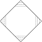
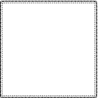
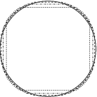
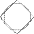
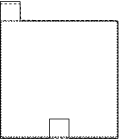
Figure 4: Evolution of contours corresponding to solutions to the equations (1.1) (upper row) and (1.2) (lower row) with the initial data $f_{S_{1}}$, $f_{S_{2}}$, $f_{S_{3}}$ and $f_{S_{4}}$, respectively.

The first two graphs in the upper row of Figure 4 present evolution of contour lines of solutions to the equation (1.1) with the initial data $f_{S_{1}}$ and $f_{S_{2}}$, respectively. In each graph, contours are plotted for the level equal to the average value of a given initial data and correspond to solutions of the equation (1.1) for $m=0$, $70$, $140$ and $210$. The contour lines of solutions to the same equation but with the initial data $f_{S_{3}}$ and $f_{S_{4}}$ and for $m=0$, $60$, $120$ and $170$ are presented in the next two graphs in the same row. The lower row of Figure 4 presents the evolution of contour lines corresponding to solutions of the equation (1.2) with the same initial data and for the same numbers of iterations as before.

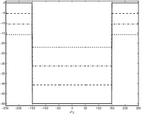
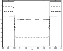
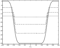
Figure 5: Evolution of numerical solutions to the equations (1.1) and (1.2) with the initial data $f_{S_{1}}$ and to the equation (1.1) with the initial data $G_{\sigma}\ast f_{S_{1}}$.

The first two plots in Figure 5 show evolution of numerical solutions to the equations (1.1) and (1.2), respectively, along cross-sectional line $x_{1}=0$ passing through the middle of the square $S_{1}$ for $m=0$, $70$, $140$ and $210$. In the case of the solution $u$ to the equation (1.1), obtained values were equal to: $\{-5.25,-40.67\}$ for $m=70$, $\{-10.5,-31.33\}$ for $m=140$, $\{-15.75,-22\}$ for $m=210$, where the first numbers in brackets correspond to values of $u$ in $\Omega\setminus S_{1}$, and the second ones, in $S_{1}$. We note that these results coincide with the exact values given by the formula (2.10) for $t=\beta\,\delta t\,m$. The third plot in Figure 5 presents the evolution of the numerical solution to the equation (1.1) for smooth initial data obtained by convolution of the image $f_{S_{1}}$ and the Gaussian kernel $G_{\sigma}$ with the standard deviation $\sigma=10$. Similarly as in the one dimensional version of the equation (1.1) studied in [20]. Here, we may observe propagation of facets.

        

        

Figure 6: In columns: (a) initial data – two binary images of the scanned text, (b) solutions to the equation (1.1), (c) solutions to the equation (1.2), (d) solutions to the linear diffusion equation.

        

        

Figure 7: Results obtained by thresholding of images presented in the lower row of Figure 6 on the level $-10$ (upper row) and on the level $-5$ (lower row).

In the last experiment, we were testing a possible application of the anisotropic total variation flow equations (1.1) and (1.2) to solve the real problem of improving the quality of the scanned text. In this experiment, we were considering two binary images presented in the first column of Figure 6 with values scaled to $\{-50,0\}$. Images in the second and third column of Figure 6 correspond to numerical solutions to the equations (1.1) and (1.2), respectively, for parameters $\gamma=10^{-2}$, $\beta=1$, $\delta t=1$, $\tau=8^{-1}$, $m=15$, and with images in the first column of Figure 6 as initial data. For comparison, in the last column of Figure 6, we present numerical solutions to the linear diffusion flow (the equation (1.2) for $\gamma=10^{-2}$, $\beta=0$, $\delta t=1$, $m=15$) with the same initial data. We observe that in fact equation (1.2) represents the interplay between an anisotropic total variation flow and the linear diffusion. It allows to fill corrupted parts of letters and at the same time slightly blur their boundaries. We notice that these properties are also visible in the results of the experiment with the image $f_{S_{4}}$, presented in the last columns of Figures 3 and 4.

In Figure 7, we present results obtained by thresholding images in the lower row of Figure 6 on the level $-10$ and $-5$, respectively. We see that application of equation (1.1) gives basically better results, however in the case when larger parts of the letters are corrupted, the properties of equation (1.2) may be useful. In general, we infer from the experiments we performed that both total variation flow models analysed in this paper provide better results when applied to a class of real problem, than the standard linear diffusion equation.

6 Appendix

Formula (2.7) must be modified in order to accommodate the boundary conditions. This is done below.

Proposition 6.1

Formula (6.1) below yields a weak solution to (1.1) in $\mathbb{R}^{2}$ with the data

$$u_{0}(x_{1},x_{2})=(x_{1}^{2}+x_{2}^{2}-2R^{2})\chi_{B(0,R)}(x_{1},x_{2})\in L^{2}(\mathbb{R}^{2}).$$

in the sense specified in Theorem 2.1. Moreover, the equation is satisfied in $\mathbb{R}^{2}$ in a pointwise manner with the exception of a one dimensional set and the solution is Lipschitz continuous, but not $C^{1}$.

Proof. Formula (2.7) shows the creation of a square facet and ruled surfaces over strips $|x_{1}|\leq\xi(t)$ and $|x_{2}|\leq\xi(t)$. Now, we have to take into account their interaction with the boundary of the ball $x_{1}^{2}+x_{2}^{2}\leq R^{2}$. The result is region $\Omega(t)$, where $u$ is different from zero. This set is defined as follows, $\Omega(t)=B(0,R)\cap(-L(t),L(t))$, where $L(t)=\sqrt{R^{2}-\xi^{2}(t)}$.

We shall see that the solution gets extinct, when the square facet hits the plane $u=0$ at $t=t_{1}$. This is why for $t\in[0,t_{1})$, we set,

$$u(x,t)=\left\{\begin{array}[]{ll}2h(t)&|x_{1}|,|x_{2}|\leq\xi(t),(x_{1},x_{2})\in\Omega(t),\\ h(t)+x_{2}^{2}-2R^{2}&|x_{1}|\leq\xi(t),\xi(t)<|x_{2}|\leq\sqrt{R^{2}-\xi^{2}(t)},(x_{1},x_{2})\in\Omega(t)\\ 0&|x_{1}|\leq\xi(t),|x_{2}|>\sqrt{R^{2}-\xi^{2}(t)},(x_{1},x_{2})\in\Omega(t),\\ h(t)+x_{1}^{2}-2R^{2}&|x_{2}|\leq\xi(t),\xi(t)<|x_{1}|\leq\sqrt{R^{2}-\xi^{2}(t)},(x_{1},x_{2})\in\Omega(t),\\ 0&|x_{2}|\leq\xi(t),|x_{1}|>\sqrt{R^{2}-\xi^{2}(t)},\\ x_{1}^{2}+x_{2}^{2}-2R^{2}&|x_{1}|,|x_{2}|>\xi(t),(x_{1},x_{2})\in\Omega(t),\\ 0&(x_{1},x_{2})\not\in\Omega(t).\end{array}\right.$$ (6.1)

This formula is valid up to $2\xi^{2}(t_{1})=R^{2}$, i.e. $t_{1}=\frac{\sqrt{2}}{6}R^{3}$.

Calculating $\nabla u$ is easy, but we have to modify ${\cal L}(\nabla u)$. Namely, we set,

$${\cal L}(\nabla u)_{1}=\left\{\begin{array}[]{ll}\frac{x_{1}}{\xi(t)}&|x_{1}|\leq\xi(t),|x_{2}|\leq\sqrt{R^{2}-\xi^{2}(t)},\\ {\rm\,sgn\,}x_{1}&|x_{1}|>\xi(t),\\ 0&|x_{2}|>\sqrt{R^{2}-\xi^{2}(t)};\end{array}\right.$$

$${\cal L}(\nabla u)_{2}=\left\{\begin{array}[]{ll}\frac{x_{2}}{\xi(t)}&|x_{2}|\leq\xi(t),|x_{1}|\leq\sqrt{R^{2}-\xi^{2}(t)},\\ {\rm\,sgn\,}x_{2}&|x_{2}|>\xi(t),\\ 0&|x_{1}|>\sqrt{R^{2}-\xi^{2}(t)}.\end{array}\right.$$

We notice that vector field ${\cal L}(\nabla u)$ has jump discontinuities, nonetheless its distributional divergence is in $L^{2}_{loc}$ and has the desired properties. It is now easy to check that $u$ satisfies (1.1) pointwise except a two-dimensional set in $\mathbb{R}^{2}\times\mathbb{R}_{+}$. We note the discontinuity of $u_{t}$ is responsible for the creation of the two dimensional facet and its growth. $\Box$

Acknowledgement

The work has been supported by the MN grant IdP2011 000661. A part of the research for this paper was performed while PR was visiting IMA, University of Minnesota, whose hospitality is acknowledged.

References

- [1] M.Alfaro, H.Garcke, D.Hilhorst, H.Matano, R.Schätzle, Motion by anisotropic mean curvature as sharp interface limit of an inhomogeneous and anisotropic Allen-Cahn equation. Proc. Roy. Soc. Edinburgh Sect. A, 140 (2010), no. 4, 673–706.
- [2] F.Andreu, C.Ballester, V.Caselles, J.M.Mazón, Minimizing total variation flow, Differential Integral Equations, 14 (2001), no. 3, 321–360.
- [3] F.Andreu-Vaillo, V.Caselles, J.M.Mazón, Existence and uniqueness of a solution for a parabolic quasilinear problem for linear growth functionals with data, Math. Ann., 322 (2002), no. 1, 139–206.
- [4] J. W. Barrett, H.Garcke, and Robert Nürnberg, Finite element approximation of one-sided Stefan problems with anisotropic, approximately crystalline, Gibbs-Thomson law, to appear in Adv. Diff. Eqs
- [5] G.Bellettini, V.Caselles, M. Novaga, The total variation flow in , J. Differential Equations, 184 (2002), no. 2, 475–525.
- [6] G.Bellettini, R.Goglione, M.Novaga, Approximation to driven motion by crystalline curvature in two dimensions. Adv. Math. Sci. Appl., 10 (2000), no. 1, 467-493.
- [7] H.Birkholz A unifying approach to isotropic and anisotropic total variation denoising models, J. Comput. Appl. Math., 235 (2011), no. 8, 2502–2514.
- [8] H.Brézis, Opŕateurs maximaux monotones et -groupes de contractions dans les espaces de Hilbert. North-Holland Mathematics Studies, No. 5. Notas de Matemática (50). North-Holland Publishing Co., Amsterdam-London; American Elsevier Publishing Co., Inc., New York, 1973.
- [9] A. Chambolle, An algorithm for total variation minimization and applications, J. Math. Imag. Vis., 20, (1-2), 2004, 89–97.
- [10] R.Choksi, Y. van Gennip, A.Oberman, Anisotropic total variation regularized approximation and denoising/deblurring of 2D bar codes. Inverse Probl. Imaging, 5 (2011), no. 3, 591-617.
- [11] P. G. Ciarlet, Introduction to numerical linear algebra and optimisation, Cambridge University Press, 1989.
- [12] I. Ekeland and R. Témam, Convex analysis and variational problems, volume 28 of Classics in Applied Mathematics. SIAM, 1999.
- [13] T. Fukui, Y.Giga, Motion of a graph by nonsmooth weighted curvature, in “World congress of nonlinear analysts ’92”, vol I, ed. V.Lakshmikantham, Walter de Gruyter, Berlin, 1996, 47-56.
- [14] W.Gao and A.Bertozzi, Level Set Based Multispectral Segmentation with Corners, SIAM J. Imaging Sci., 4 (2011), no. 2, 597–617.
- [15] Y.Giga, H.Kuroda, N.Yamazaki, Global solvability of constrained singular diffusion equation associated with essential variation, in Free boundary problems, Internat. Ser. Numer. Math., 154, Birkhäuser, Basel, 2007, 209-218.
- [16] H.-Y.Huang, Ch.-Y.Jia, Z.-D.Huan, On weak solutions for an image denoising-deblurring model, Appl. Math. J. Chinese Univ. Ser. B , 24 (2009), no. 3, 269–81.
- [17] K. Kielak, P.B. Mucha, P. Rybka, Almost classical solutions to the total variation flow. J. Evol. Eqs, 13, (2013), 21–49.
- [18] J.S.Moll, The anisotropic total variation flow, Math. Ann., 332, No. 1, 177-218 (2005).
- [19] P.B. Mucha, Regular solutions to a monodimensional model with discontinuous elliptic operator, Interfaces Free Bound, 14 (2012), no. 2, 145–152.
- [20] P.B. Mucha, P. Rybka, A Note on a Model System with Sudden Directional Diffusion J. Stat. Phys., 146, no 5, (2012) 975-988.
- [21] P.B. Mucha, P. Rybka, Well-posedness of sudden directional diffusion equations, Math. Methods Applied Sci., DOI: 10.1002/mma.2759
- [22] T.Preusser, Viscosity Solutions of a Level-Set Method for Anisotropic Geometric Diffusion in Image Processing, J. Math. Imaging Vis., 29 (2007), 205–217.
- [23] L. Rudin, S. Osher and E. Fatemi, Nonlinear total variation based noise removal algorithms, Physica D, , 60, (1992), 259–268.
- [24] H. Spohn, Surface dynamics below the roughening transition, J. de Physique I, 3, (1993), 68-81.
- [25] Y.-H.R.Tsai, S.Osher, Total variation and level set methods in image science, Acta Numerica, 14, (2005), 509-573.