Reconstruction and constraining of the jerk parameter from OHD and SNe Ia observations

Abstract

Compared with the plentiful researches of the Hubble parameter and deceleration factor, the third time derivative of the scale factor $a(t)$ in the FRW cosmology, namely, the jerk parameter $j$ still lacks attention. In order to study the properties of $j$, we propose several kinds of parameterizations of $j(z)$ as a function of the redshift $z$. By setting the standard $\Lambda$CDM model as the fiducial model, we constrain the jerk models with the observational Hubble parameter data (OHD) and Type Ia Supernovae (SNe) observations. We find that the perturbation of $j(z)$ favors a value of nearly zero and the $\Lambda$CDM is well accommodated by the jerk reconstruction. We also compare the powers of OHD and SNe in constraining the jerk models in detail, and find that the newly released OHD measurement at $z=2.3$ can improve the constraint significantly, even tighter than the SNe one. Furthermore, we analyze the jerk models by calculating the Hubble parameter, equation of state, the deceleration factor and $Om(z)$ diagnostic. Our results show that the universe is indeed undergoing an accelerated expansion phase following the matter-dominated one, which is consistent with the standard model by observations.

I Introduction

One of the most important discoveries of the modern cosmology is the accelerated expansion of the universe. This phenomenon was first discovered by the type Ia supernovae observations SNe..Riess ; SNe..Hicken ; SNe..Perlmutter , and later further confirmed by the measurements of the cosmic microwave background (CMB) CMB..Spergel ; CMB..Komatsu , the baryon acoustic oscillation (BAO) BAO..Eisenstein ; BAO..Percival and so on. Now more than ten years later, this phenomenon has been accepted widely. As pointed out in Ref.review..Weinberg , the question concerning this is no longer whether the universe is accelerating, but why.

In order to give a reasonable explanation to this scenario, a great variety of attempts have been done. These works include the dark energy models which involve the introduction of exotic matter sources, and the modified gravity models which relates to the changes of the geometry of the spacetime dark..energy..review..Tsujikawa ; dark..energy..review..Sola ; dark..energy..review..Li ; dark..energy..review..Capozziello ; dark..energy..review..Trodden . Although these models can solve some problems and fit the observational data, they also have their own difficulties. For example, the standard $\Lambda$CDM model is considered to be the simplest and most natural one which shows great consistence with the observational dataLCDM..Jassal ; LCDM..Wilson ; LCDM..Davis ; LCDM..Allen . In this model, the cosmological constant $\Lambda$ is considered to be the dark energy component of the universe. However, it is also challenged by the fine-tuning problem and the coincidence problem. So the study of explaining the accelerated expansion is still continued and the new models are being proposed cons..prob..S..Weinberg ; cons..pro..A. Vilenkin ; cons..pro..J. Garriga ; cons..pro..G. Caldera-Cabral .

For obtaining more information of the evolutionary behavior of the universe, one can study the time derivative of the scale factor $a(t)$ with respect to the redshift $z$ in the frame of a FRW universe, such as the Hubble parameter $H=\dot{a}/a$, the deceleration factor $q=-\ddot{a}/(aH^{2})$ and so on. As a direct indication of the decelerated/accelerated expansion, the parameter $q$ has been studied from both the observational and theoretical views, including the constraints from the observational data, the analysis of a particular model, or the reconstruction by some statistical methods such as the Principle Component Approach (PCA) and so on q..Cunha ; q..Virey ; q..Yi ; q..Otto ; PCA..Huterer ; q..Shapiro ; q..Campo . As a higher order derivative of the scale factor, the jerk parameter $j=-\dddot{a}/(aH^{3})$ is related to the third time derivative of $a$ (we notice that in some earlier works, there is no negative sign in the definition as Ref.j..Blandford ; j..Visser and so forth. However, some literatures contain the negative sign as Ref.j..model2..1 ; j..model2..2 . We point out the difference here in order to avoid the confusion). It is a measurement of the variation of $q$ and can be used as an indication to predict the future of the universe. Because the higher-order derivatives can characterize the dynamics of the universe, it could be related to the emergence of sudden future singularities future..Dabrowski ; future..Dabrowski2 . Another example is the $\Lambda$CDM cosmology where $j_{\Lambda}=-1$ implies that the universe will continue to expand with an acceleration because of the cosmological constant. Except that, the jerk parameter $j$ is also applied in the statefinder diagnostic to discriminate different dark energy or modified gravity models statef..Sahni ; statef..Alam ; j..fR ; j..Dunajski ; j..Poplawski . Although the single $j$ can not identify some similar models as $\Lambda$CDM and Einstein de-Sitter universe, its combination with $q$ can comprise an identification in a wider range of cosmological models. Compared with the plentiful research works of $q$, the jerk parameter has not been fully explored at present j..Xu ; j..Xu2 ; j..Lu ; j..model2..1 ; j..model2..2 ; j..Rapetti ; j..first . It is therefore natural to study the jerk parameter because of its importance in cosmology.

Among the numerous cosmological models, the standard $\Lambda$CDM model can fit most of the observations and is considered as the best oneLCDM..Maor ; LCDM..Basilakos ; dark..energy..review..Tsujikawa . Thus, it is reasonable to set the $\Lambda$CDM model as the fiducial model and thus $j=-1$ is an important reference. In our calculation, we will mainly measure the departure of $j$ from -1 by its parameterizations. This will be a direct generalization of the standard $\Lambda$CDM model. Specifically, we will reconstruct jerk as $j(z)=-1+departure$ and measure the departure term with the observational data. The results can give us the impression if the universe in the past was strictly the standard model or not.

In our work, the constraints on $j$ are presented by the use of the latest Union 2.1 supernovae data (SNe) Union2.1..Suzuki and the observational Hubble parameter data (OHD) OHD..Farooq . As the two widely used measurements at low redshift, SNe and OHD have been applied in dozens of cosmological researches OHD..Farooq ; OHD..ChenY ; SNe..Mueller ; SNe..Lu ; SNe..Grande ; OHD..Basilakos ; OHD..ZhangH ; OHD..Duan ; OHD..Liao ; OHD..Cao ; OHD..Cao2 ; SNe..Godlowski ; OHD..Lazkoz ; OHD..Wei ; OHD..Wu ; OHD..Kurek ; SNe..ZhangX . The comparisons between them were also discussed deeply and widely OHD..Ma ; OHD..ZhangT ; OHD..Zhai ; OHD..Lin . Therefore, we also compare the powers of SNe and OHD in constraining the models of jerk parameterizations and analyze the differences between them.

Our paper is organized as follows: In Sec. II, the basic formulas of the kinematical models and the reconstruction of jerk parameter are presented. In Sec.III, the constraints by use of SNe and OHD data sample are obtained and analyzed. Our discussions and conclusions are given in Sec.IV.

II Kinematical models and the constraints

II.1 Reconstruction of $j(z)$

Let’s start with the Friedmann-Robertson-Walker (FRW) metric which describes a homogenous and isotropic universe

$$ds^{2}=-dt^{2}+a^{2}(t)\left[\frac{dr^{2}}{1-kr^{2}}+r^{2}d\Omega^{2}\right],$$ (1)

where $k$ is the spatial curvature and for simplicity, we hereafter will assume it to be zero, namely, our calculation will be carried out in a spatial flat FRW universe CMB..Komatsu . And the function $a(t)$ is the scale factor and its current value is always set to be unity, therefore the time recording of the history of the universe can be represented by the redshift $z$ with the relation $a=(1+z)^{-1}$.

As mentioned in the preceding section, the time derivatives of $a$ are defined as

$$H(z)\equiv\frac{\dot{a}}{a},$$ (2)

$$q(z)\equiv-\frac{1}{H^{2}}\frac{\ddot{a}}{a}=\frac{1}{2}(1+z)\frac{[H(z)^{2}]^{\prime}}{H(z)^{2}}-1,$$ (3)

$$j(z) \equiv-\frac{1}{H^{3}}\frac{\dddot{a}}{a}=$$ (4)

$$-\left[\frac{1}{2}(1+z)^{2}\frac{[H(z)^{2}]^{\prime\prime}}{H(z)^{2}}-(1+z)\frac{[H(z)^{2}]^{\prime}}{H(z)^{2}}+1\right],$$

where the prime denotes the derivative with respect to the redshift $z$.

Within the assumption of a constant $j(z)$, Eq.(4) is an Euler equation solved as

$$H^{2}(z)=\tilde{C_{1}}(1+z)^{\alpha_{+}}+\tilde{C_{2}}(1+z)^{\alpha_{-}},$$ (5)

where $\tilde{C_{1}}$ and $\tilde{C_{2}}$ are arbitrary constants and

$$\alpha_{\pm}=\frac{3\pm\sqrt{1-8j}}{2}.$$ (6)

The solution gives a constraint that $j<0.125$. With the redefinition of $C_{1,2}=\tilde{C}_{1,2}/H_{0}^{2}$, where the subscript ’0’ stands for the current value of a quantity, the expansion factor of the FRW cosmology can be written as

$$E(z)=\frac{H(z)}{H_{0}}=(C_{1}(1+z)^{\alpha_{+}}+C_{2}(1+z)^{\alpha_{-}})^{\frac{1}{2}}.$$ (7)

Then using the definition of the expansion factor $E(z)=H(z)/H_{0}$, we can substitute $E(z)$ into Eq.(4) and replace $H(z)$ without any essential change.

In order to determine the constants appeared in Eq.(7) and their physical meanings in the solution, we can apply a particular cosmological model as a reference. In the $\Lambda$CDM model, we have $j=-1$ and Eq.(7) becomes

$$E(z)=(C_{1}(1+z)^{3}+C_{2})^{\frac{1}{2}}.$$ (8)

It is clear that $C_{1}$ becomes the matter term $\Omega_{m0}$ (including the ordinary matter and the dark matter) and $C_{2}$ represents the cosmological constant term $\Omega_{\Lambda}$. However, we should notice that this correspondence is just valid in the frame of the $\Lambda$CDM model. We can not say for sure the explicit relationship between $C_{1}$, $C_{2}$ and $\Omega_{m0}$, $\Omega_{\Lambda}$, but the approximation of $\Lambda$CDM model is a proper reference for us to find the real meaning of the parameters $C_{1}$ and $C_{2}$. Additionally, the current value of Eq.(7) gives

$$C_{1}+C_{2}=1.$$ (9)

The assumption of $j=constant$ leads Eq.(4) to a homogeneous Euler equation which can be seen more obviously under the variable substitutions:

$$(1+z)\rightarrow x,\qquad H^{2}\rightarrow y(x).$$ (10)

This result provides us the possibility to test the deviation of $j(z)$ from -1 or other value in the past, but the calculation is dependent on the functional form of $j(z)$. Similarly as the methods studying the properties of the interaction between dark energy and dark matter by assuming some phenomenological models interaction..Cai , one possible proposal in reconstructing jerk is

$$j(z)=j_{0}+j_{1}\frac{f(z)}{E^{2}(z)},$$ (11)

where $j_{0}$ and $j_{1}$ are constants needed to be constrained while $f(z)$ is an arbitrary function of redshift $z$, the different choices of which can lead to different reconstructions of $j(z)$.This kind of assumption has several advantages. Firstly, it can make Eq.(4) analytically solvable under particular models of $f(z)$. Secondly, it can also make Eq.(4) more symmetric by satisfying both sides of the equation comprised by a constant term plus a $E^{-2}$ term.

The simplest form of $f(z)$ is perhaps the linear form which can be written as $f(z)=z$, which is the first order of the linear expansion of $f(z)$. Moreover, inspired by reconstructing the equation of state (EoS) of the dark energy, we propose another model similarly as the CPL parameterizations CPL..Chevallier ; CPL..Linder

$$f(z)=(1-a)=\frac{z}{1+z}.$$ (12)

To be more general, we can also apply some functions which are different from the above. We choose the similar JBP JBP..Jassal (in reconstructing the EoS of dark energy) and the logarithmic model. To sum up, we apply four models of $f(z)$ in our calculation. Moreover, as mentioned in the previous section, we regard the standard $\Lambda$CDM model as the fiducial model and reconstruct $j(z)$ aiming at measuring the departure of $j$ from -1. Therefore $j_{0}$ in Eq.(11) can be set to -1 and the second term can be seen as the perturbation. This thought is similar with the previous work j..Rapetti , but the specific method is different. The authors there adopted the Chebyshev polynomials in reconstructing $j(z)$ and presented a detailed analysis. In our calculation, we just parameterize the $j(z)$ phenomenologically and make the Euler equation solvable. Once the above reconstructing methods are introduced, we can summarize the four parameterizations as

Model I $$j(z)=-1+j_{1}\frac{z}{E^{2}(z)}$$ (13)

Model II $$j(z)=-1+j_{1}\frac{z}{1+z}\frac{1}{E^{2}(z)}$$ (14)

Model III $$j(z)=-1+j_{1}\frac{z}{(1+z)^{2}}\frac{1}{E^{2}(z)}$$ (15)

Model IV $$j(z)=-1+j_{1}\frac{\ln(1+z)}{E^{2}(z)}.$$ (16)

One point worth noticing is that all these models have $j(z=0)=-1$. More discussions of this issue will be given in the following section. Substituting these equations into Eq.(4), we can obtain the solutions of $E(z)$

Model I $$E^{2}(z)=\frac{1}{3}C_{1}(1+z)^{3}+C_{2}+j_{1}(1+z)-\frac{2}{3}j_{1}\ln(1+z)$$ (17)

Model II $$E^{2}(z)=\frac{1}{3}C_{1}(1+z)^{3}+C_{2}+\frac{j_{1}}{2(1+z)}+\frac{2}{3}j_{1}\ln(1+z)$$ (18)

Model III $$E^{2}(z)=\frac{1}{3}C_{1}(1+z)^{3}+C_{2}+\frac{j_{1}}{5(1+z)^{2}}-\frac{j_{1}}{2(1+z)}$$ (19)

Model IV $$E^{2}(z)=\frac{1}{3}C_{1}(1+z)^{3}+C_{2}+\frac{2}{9}j_{1}\ln(1+z)+\frac{1}{3}j_{1}\ln^{2}(1+z).$$ (20)

The coefficients $C_{1}$ and $C_{2}$ arise from the process of solving Eq.(4) which is a second order differential equation. Another constraint that $E(z=0)=1$ gives a relationship between the constants $C_{1}$, $C_{2}$ and $j_{1}$

Model I $$C_{2}=1-j_{1}-\frac{1}{3}C_{1}$$ (21)

Model II $$C_{2}=1-\frac{j_{1}}{2}-\frac{1}{3}C_{1}$$ (22)

Model III $$C_{2}=1+\frac{3}{10}j_{1}-\frac{1}{3}C_{1}$$ (23)

Model IV $$C_{2}=1-\frac{1}{3}C_{1}$$ (24)

Thus each model above has two free parameters ($C_{1},j_{1}$) needed to be constrained by the observational data.

II.2 Observational data

The first observational data sample used in our calculation is the measurements of Type Ia Supernovae (SNe Ia). This kind of observation plays an important role in discovering the accelerated expansion of the universe. Its application in constraining the cosmological models comes from the distance modulus which is defined as

$$\mu(z)=5\log(d_{L}/Mpc)+25,$$ (25)

where $d_{L}$ is the luminosity distance. In a spatially flat FRW universe, the luminosity distance of a cosmological source at redshift $z$ reads as

$$d_{L}=(1+z)\int_{0}^{z}\frac{dz^{\prime}}{H(z^{\prime})}.$$ (26)

The parameters introduced in the model can be obtained through the $\chi^{2}$ statistics. In our calculations, we choose the marginalized nuisance parameter SNe..Nesseris for $\chi^{2}$

$$\chi^{2}_{\text{SNe}}=A-\frac{B^{2}}{C}$$ (27)

where

$$A=\sum_{i}\frac{[\mu_{obs}(z_{i})-\mu_{th}(z_{i})]^{2}}{\sigma_{i}^{2}},$$ (28)

$$B=\sum_{i}\frac{[\mu_{obs}(z_{i})-\mu_{th}(z_{i})]}{\sigma_{i}^{2}},$$ (29)

$$C=\sum_{i}\frac{1}{\sigma_{i}^{2}},$$ (30)

where $\sigma_{i}$ denotes the $1\sigma$ uncertainty of the $i$th measurement. The subscripts “obs” and “th” stand for the observational and theoretical values of a variable respectively. In our work, we choose the latest Union2.1 compilation of the SNe data sample Union2.1..Suzuki which contains 580 Type Ia supernovae observations in the redshift range $0<z<1.414$. On the other hand, the systematic errors in measuring the luminosity distance should also be considered. Thus we calculate the constraints of Union2.1 with systematic errors of the jerk parameterizations as well. The method we used here is the same as suggested in Ref.OHD..Farooq .

We also adopt the observational Hubble parameter data (OHD) in our constraints. It is known that the SNe is powerful in constraining the cosmological models. However, the integration in its formula makes it hard to reflect the precise evolution of $H(z)$. Therefore, the fine structure of the expansion history of the universe can be well indicated by the $H(z)$ data. The measurement of OHD can be derived from the differential of redshift $z$ with respect to the cosmic time $t$

$$H(z)=-\frac{1}{1+z}\frac{dz}{dt}.$$ (31)

In this work, we use the 21 $H(z)$ measurements of Ref. OHD..Jimenez ; OHD..Jimenez2 ; OHD..Simon ; OHD..Stern2 ; OHD..Gaztanaga ; OHD..Moresco to constrain the jerk models.

The $\chi^{2}$ value for the OHD can be expressed as

$$\chi^{2}_{\text{OHD}}=\sum_{i=1}^{21}\frac{[H_{obs}(z_{i})-H_{th}(z_{i})]^{2}}{\sigma_{i}^{2}}.$$ (32)

The best-fit values of the parameters can be obtained by minimizing the above quantity. It should be noticed that there is a nuisance parameter in the OHD constraint: $H_{0}$. Therefore, we marginalize it by using a prior $H_{0}=74.3\pm 2.1$ km s^-1 Mpc^-1 OHD..Freedman which contains a 2.8% systematic uncertainty. On the other hand, the prior value of $H_{0}=68\pm 2.8$km s^-1 Mpc^-1 was also used in the previous works and showed efficient constraints on the cosmological modelsOHD..Chen . Except that, this value is more consistent with the newly released Planck resultsPlanck . So we also use this prior in our calculation and the results may provide valuable comparisons.

Additionally, as the newly measurement at $z=2.3$ from the Baryon Acoustic Oscillation (BAO) in the Ly$\alpha$ is discovered OHD..Busca , we also adopt this data in our calculation in order to find the effect of this addition in constraining cosmological models. For convenience, we will use the term ”$H_{2.3}$” in the following sections to denote this measurement.

III Constraint results

Figure 1: The confidence regions of $(j_{1},C_{1})$ obtained from SNe with (solid) and without (dotted) systematic errors respectively. The 68.3%, 95.4% and 99.7% confidence level are presented from inner to outer. The thin (without systematic errors) and thick circles (with systematic errors) stand for the best-fit values.

	data	$j_{1}$	$C_{1}$	$\chi_{\text{min}}^{2}$	FoM
Model I	SNe a	$0\pm 2.14$	$0.84\pm 0.60$	$561.73$	7.7829
Model I	SNe b	$0\pm 3.68$	$0.88\pm 1.05$	$545.84$	2.0923
Model II	SNe a	$0\pm 2.96$	$0.84\pm 0.37$	$561.73$	5.5381
Model II	SNe b	$0.4\pm 5.14$	$0.84\pm 0.62$	$545.83$	1.4662
Model III	SNe a	$0\pm 4.03$	$0.84\pm 0.27$	$561.73$	4.1031
Model III	SNe b	$-0.4\pm 7.56$	$0.92\pm 0.49$	$545.84$	1.0994
Model IV	SNe a	$0\pm 2.45$	$0.81\pm 0.41$	$561.73$	6.5553
Model IV	SNe b	$0.2\pm 4.49$	$0.86\pm 0.76$	$545.83$	1.7271

Table 1: The constraint results of the parameters from SNe sample, including the best-fit values with $1\sigma$ errors of the parameters and the FoM of four jerk parameterizations. (the subscript $a$: without systematic errors; $b$: with systematic errors.)

Figure 2: The confidence regions of $(j_{1},C_{1})$ obtained from OHD with $H_{0}$ priors of $H_{0}=74.3\pm 2.1$ km s^-1 Mpc^-1 (dotted) and $H_{0}=68\pm 2.8$ km s^-1 Mpc^-1 (solid) respectively. The 68.3%, 95.4% and 99.7% confidence level are presented from inner to outer. The thin ($H_{0}=74.3\pm 2.1$ km s^-1 Mpc^-1) and thick circles ($H_{0}=68\pm 2.8$ km s^-1 Mpc^-1) stand for the best-fit values.

	data	$j_{1}$	$C_{1}$	$\chi_{\text{min}}^{2}$	FoM
Model I	OHD (H${}_{0}^{\prime}$)	$-2.0\pm 1.63$	$1.19\pm 0.36$	$20.65$	5.8160
Model I	OHD (H0)	$0.4\pm 2.02$	$0.88\pm 0.42$	$19.85$	3.5082
Model II	OHD (H${}_{0}^{\prime}$)	$-3.3\pm 2.60$	$1.04\pm 0.24$	$20.44$	3.7051
Model II	OHD (H0)	$0.4\pm 3.35$	$0.92\pm 0.27$	$19.85$	2.2067
Model III	OHD (H${}_{0}^{\prime}$)	$-5.3\pm 3.92$	$0.97\pm 0.18$	$20.27$	2.4601
Model III	OHD (H0)	$0.8\pm 4.99$	$0.92\pm 0.19$	$19.86$	1.4410
Model IV	OHD (H${}_{0}^{\prime}$)	$-2.6\pm 2.06$	$1.09\pm 0.28$	$20.53$	4.5895
Model IV	OHD (H0)	$0.4\pm 2.64$	$0.92\pm 0.32$	$19.85$	2.7454

Table 2: The constraint results of the parameters from OHD sample, including the best-fit values with $1\sigma$ errors of the parameters and the FoM of four jerk parameterizations. ($H_{0}^{\prime}$ denotes the value $74.3\pm 2.1$ km s^-1 Mpc^-1 of the prior is used, while $H_{0}$ denotes $68\pm 2.8$ km s^-1 Mpc^-1 is applied.)

Figure 3: The confidence regions of $(j_{1},C_{1})$ obtained from OHD+H_2.3 with $H_{0}$ priors of $H_{0}=74.3\pm 2.1$ km s^-1 Mpc^-1 (dotted) and $H_{0}=68\pm 2.8$ km s^-1 Mpc^-1 (solid) respectively. The 68.3%, 95.4% and 99.7% confidence level are presented from inner to outer. The thin ($H_{0}=74.3\pm 2.1$ km s^-1 Mpc^-1) and thick circles ($H_{0}=68\pm 2.8$ km s^-1 Mpc^-1) stand for the best-fit values.

	data	$j_{1}$	$C_{1}$	$\chi_{\text{min}}^{2}$	FoM
Model I	OHD+$H_{2.3}$ (H${}_{0}^{\prime}$)	$-0.3\pm 0.87$	$0.79\pm 0.22$	$22.24$	17.488
Model I	OHD+$H_{2.3}$ (H0)	$1.2\pm 1.11$	$0.70\pm 0.15$	$20.30$	10.5487
Model II	OHD+$H_{2.3}$ (H${}_{0}^{\prime}$)	$-0.8\pm 1.60$	$0.78\pm 0.09$	$22.12$	9.8872
Model II	OHD+$H_{2.3}$ (H0)	$1.6\pm 2.31$	$0.80\pm 0.11$	$20.41$	5.8390
Model III	OHD+$H_{2.3}$ (H${}_{0}^{\prime}$)	$-1.6\pm 2.64$	$0.77\pm 0.07$	$21.98$	6.0180
Model III	OHD+$H_{2.3}$ (H0)	$3.2\pm 3.35$	$0.80\pm 0.07$	$20.52$	3.4702
Model IV	OHD+$H_{2.3}$ (H${}_{0}^{\prime}$)	$-0.5\pm 1.21$	$0.78\pm 0.10$	$22.18$	12.9475
Model IV	OHD+$H_{2.3}$ (H0)	$1.6\pm 1.55$	$0.74\pm 0.10$	$20.38$	7.6735

Table 3: The constraint results of the parameters from OHD+H_2.3 sample, including the best-fit values with $1\sigma$ errors of the parameters and the FoM of four jerk parameterizations.($H_{0}^{\prime}$ denotes the value $74.3\pm 2.1$ km s^-1 Mpc^-1 of the prior is used, while $H_{0}$ denotes $68\pm 2.8$ km s^-1 Mpc^-1 is applied.)

III.1 Constraints from SNe and OHD

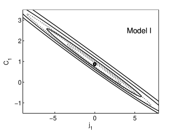
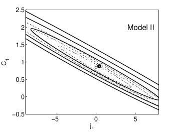
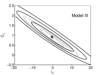
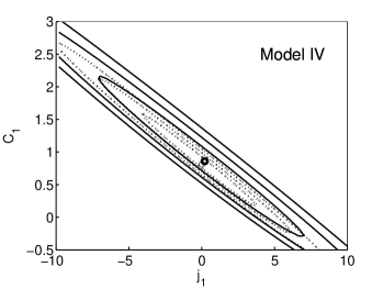
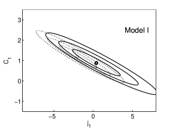
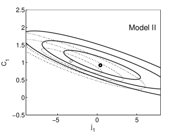
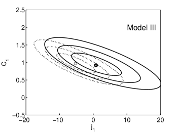
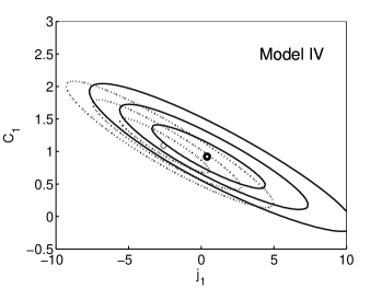
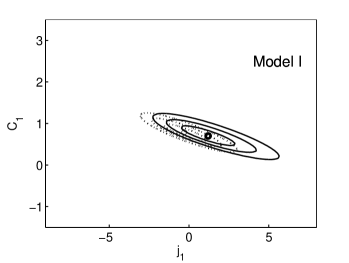
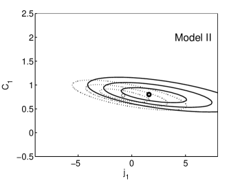
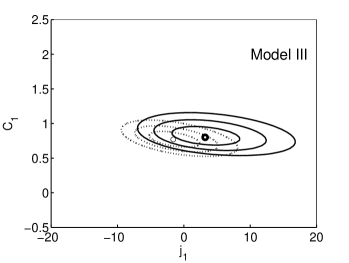
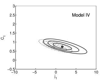
Our constraint results are presented in Fig.1 and Fig.2where the $1\sigma$, $2\sigma$ and $3\sigma$ confidence regions are shown. These are obtained by finding the contours of $\chi^{2}_{min}+2.3,6.17,11.8$ in the parameter space respectively. Also, we summarize the best-fit values and the corresponding uncertainties of the parameters in Table.1 and Table.2. From these results, we can see that the $\Lambda$CDM model or the $j(z)=-1$ model is well accommodated by supernovae observations (with and without systematic errors). The best-fit values of $j_{1}$ in four jerk models are very small which imply that the perturbation term in Eq.(13)-(16) can be ignored. Therefore, the standard $\Lambda$CDM model is well preferred by SNe data. The difference between the samples considering and not considering systematic errors is also obvious. The constraints from the former ones are apparently looser than the latter ones. The 2$\sigma$ confidence regions of SNe not considering systematic errors is almost overlap with the 1$\sigma$ confidence regions of considering systematic errors ones. This situation is expectable since the consideration of the systematic errors means the reduction of the accuracy of the information we obtained. And this can be well reflected by the confidence regions of the parameters.

On the other hand, the OHD constraints show different results about $\Lambda$CDM model. All the four jerk models indicate a tendency of deviation of the universe from the $\Lambda$CDM model. The best-fit values of $j_{1}$ given by OHD are less than zero and can not be neglected when the first prior $H_{0}=74.3\pm 2.1$ km s^-1 Mpc^-1 is used . Moreover, these situation appears in all the four models. However, the choice of the second prior $H_{0}=68\pm 2.8$ km s^-1 Mpc^-1 changes the above situation. All the four jerk models show the best-fit values of $j_{1}\geq 0$. These results are more consistent with the SNe ones. But we should notice that the second prior of $H_{0}$ gives worse constraints of the parameters than the first one.

Based on these results, we can hardly say that the OHD and SNe give very different constraints because the uncertainties should be taken into account. The confidence regions of these two data samples show the overlap at certain confidence level and this phenomenon can be seen as a signal that the OHD and SNe can give similar constraints. In particular, the best-fit values of the constraint from one data sample can locate in the 1$\sigma$ confidence region using different sample. Except that, the tendencies of the confidence regions given by these two data samples are very similar. Therefore, the present results approve the previous works that the OHD can play the same role as SNe in constraining cosmological models OHD..Zhai ; OHD..Lin .

An important point worth noticing is the differences of the powers of OHD and SNe in constraining the cosmological models. In the jerk parameterizations, the OHD shows that the uncertainties of the parameters are smaller than the SNe ones. Thus we may conclude that the OHD is more powerful than SNe. Because of the smaller size of OHD sample, this is quite a satisfactory phenomenon. However, looking at the confidence regions, we find that the constraints given by OHD are not as strict as the SNe ones.

Except for the uncertainties of the parameters, the size of the confidence region at certain level is another useful tool in evaluating the powers of observational data in constraining cosmological models. In order to compare the abilities of OHD and SNe in constraining the jerk models quantitatively, we adopt the test of Figure of Merit (FoM). Similarly, we choose the definition of FoM as the Dark Energy Task Force (DETF) used FoM..Albrecht ; FoM..Huterer . The FoM is the inverse of the area of the 95.4% confidence level region $A_{95}$ in the parameter space (the $j_{1}-C_{1}$ plane in our models.). Once the normalization is considered, we define FoM as FoM..Mortonson ; FoM..Ruiz

$$\text{FoM}_{(j_{1},C_{1})}\approx\frac{6.17\pi}{A_{95}}.$$ (33)

If the probability distribution of the parameter is Gaussian, the approximate equality in this equation becomes exact.

The FoM results are summarized in the rightmost column of Table.1,Table.2 and Table.3. We find that the FoM test does not clearly approve the above conjecture that OHD is superior than SNe. The FoM of SNe without considering the systematic errors is about 1.5 times of the OHD ones. But the addition of the systematic errors changes this because its FoM is smaller than OHD. Thus in fact, the constraints in all the four models show that the powers of OHD and SNe in constraining cosmological models are hard to evaluate because their FoM values are sensitive to the choice of systematic errors. About the Hubble parameter data themselves, their constraints are also sensitive to the choice of the prior. The second prior $H_{0}=68\pm 2.8$ km s^-1 Mpc^-1 gives worse constraints as we mentioned in the previous paragraphs.

We can conclude that the SNe data give both larger uncertainties of the parameters and strict constraint. This seems to be paradoxical but in fact not, because it reflects that the correlations of the parameters given by OHD is weaker than SNe gives. In other words, the parameters in OHD are more independent between each other FoM..Coe .

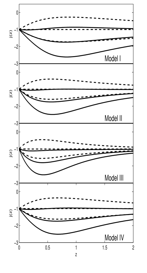
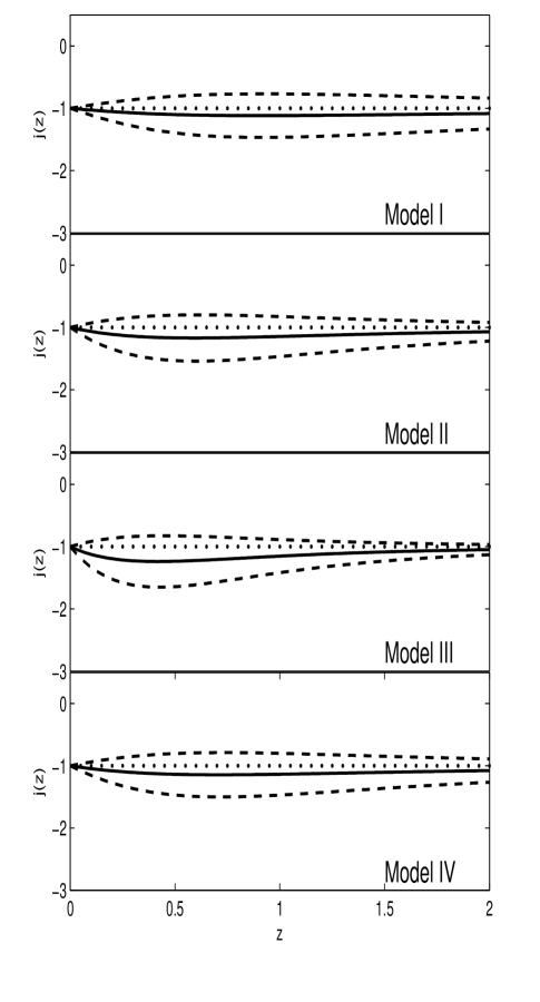
The reconstructions of $j(z)$ of the jerk models are plotted in the left panel of Fig.4 as illustrations (The best-fit values and errors of the parameters are chosen by SNe (without systematic errors) and OHD (first prior)). The SNe data strongly favor the $\Lambda$CDM model, while the OHD prefers a deviation. Once the uncertainties are considered, this deviation disappeared. The curve of standard $\Lambda$CDM model evolves almost along the boundary of the $1\sigma$ confidence level.

Figure 4: The reconstruction of jerk parameter. $Left$: The dotted and solid lines represent the best-fit and $1\sigma$ error curves of SNe and OHD respectively. Right: The results obtained from OHD+H2.3 including the best-fit value and 1$\sigma$ error. The dots stand for j(z) = -1 line.

III.2 The addition of $H_{2.3}$

Recently, the new OHD measurement at $z=2.3$ from BAO in Ly$\alpha$ was discovered with the value of $H(z=2.3)=224\pm 8$ km s^-1 Mpc^-1 OHD..Busca . This measurement has been used in constraining cosmological models OHD..Farooq2 and shows that the addition of it can provide restrictive constraint. In particular, the constraints are tighter than those from SNe data OHD..Farooq2 . This should be attributed to the high redshift of this measurement and the apparently small uncertainty which has been carefully estimated. This can naturally increase its weight in the $\chi^{2}$ statistics.

In our calculation, we also adopt this measurement to the OHD sample. The constraint results of the jerk parameterizations are presented in Fig.3. The best-fit values and the uncertainties of the parameters are also summarized in Table.3. We can find that similarly, the addition of $H_{2.3}$ improves the constraints apparently. This can be obtained from both the uncertainties and FoM test, even it can help OHD to provide tighter constraints than SNe data. The values of FoM based on OHD are almost double of that from SNe, which is a significant progress and is consistent with the previous work OHD..Farooq2 . Also, the best-fit values of the parameters show a preference to the $\Lambda$CDM model, where the absolute value of $j_{1}$ reduces. Taking into account of the uncertainties, we find that OHD+H_2.3 give more consistent constraints compared with the SNe ones

The reconstruction of $j(z)$ are plotted in the right panel of Fig.4 (parameters applied are the same as left panel). It can be found that the standard $\Lambda$CDM model is apparently favored by OHD+H_2.3. Additionally, the $1\sigma$ error of the reconstruction is also reduced even smaller than the SNe ones. It is anticipated that OHD+H_2.3 provides tighter and more efficient constraint than SNe.

Except that, we can see that all the data samples including SNe, OHD and OHD+H_2.3 show that $j(z)$ goes to -1 as the redshift $z$ increase. This is natural as we go back along the cosmic evolution there was a matter-dominated phase before the current accelerated expansion. The Hubble parameter can be approximated as

$$H^{2}(z)\approx\Omega_{m0}(1+z)^{3}.$$ (34)

Substituting this equation into Eq.(4), we may find the first two terms in the bracket of the right hand side cancel out and just leave $j(z)=-1$. Perhaps this can be treated as a criteria in reconstructing $j(z)$ because the matter-dominated phase is almost a necessity.

III.3 The Hubble parameter and the equation of state

Figure 5: $Left$: The evolution of the Hubble parameter $H(z)$ with respect to the redshift $z$. The solid curves represent the best fit results of OHD+H_2.3 while the dashed lines stand for the 1$\sigma$ errors. The original data points are also shown. $Right$: The reconstruction of the equation of state as a function of the redshift $z$ by the use of the OHD+H_2.3 results. The solid lines and dashed lines stand for the best-fit results and 1$\sigma$ errors respectively. The dotted lines represent the $\Lambda$CDM case.

As we know, the jerk parameter relates to the third time derivative of the scale factor. Although $j(z)$ is a good function to describe the evolution of the universe, to identify different dark energy models as a part of the so-called ”statefinder” diagnostic, to study the future including the type of the singularities of the universe future..Dabrowski ; future..Dabrowski2 ; future..Astashenok ; future..Frampton ; future..Frampton2 and so forth, its dynamical properties are not easily handled, at least not as obvious as the deceleration factor or the Hubble parameter. In order to study the effects of our reconstructions of $j(z)$ and trace its behavior, we calculate the Hubble parameter and the equation of state in this section.

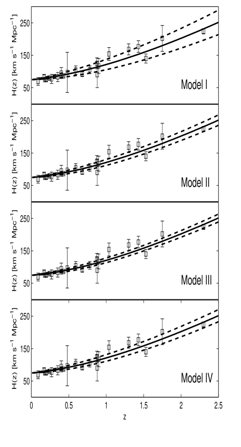
In the left pannel of Fig.5, we plot the evolution of the Hubble parameter $H(z)$ of the jerk models by the use of OHD+H_2.3. The original data points are also shown in the same plane for comparison. The importance of H_2.3 is also clear because the whole point (with error bar) locates in the 1$\sigma$ errors of $H(z)$.

As another important parameter, the equation of state $\omega$ of the “dark energy” plays a crucial role in explaining the cosmic acceleration. On the other hand, $j(z)$ can be also interpreted in fluid term through the relationj..Blandford

$$j=-1+\frac{4\pi\dot{P}}{H^{3}},$$ (35)

where $P$ is the pressure and the gravitational constant $G$ is set to be unity. This expression is valid without considering the spatial curvature. Moreover, this equation derives the relation between $j$ and $w$ as in Ref.j..Blandford where a constant $w$ is assumed. It is also interesting to calculate $w$ in our jerk parameterizations. If we assume that matter evolves in the usual way, the first term in the expression of $E(z)$ in Eq.(17)-(20) can be treated as the matter term with $C_{1}/3=\Omega_{m0}$, while the rests stand for the “dark energy” term. Specifically, the models can be summarized as

$$E^{2}(z)=\Omega_{m0}(1+z)^{3}+\Omega_{DE}(z),$$ (36)

where the subscript “DE” represents the dark energy term. On the other hand, from the Friedmann equation, we can obtain $E(z)$ in a universe comprised by the matter and exotic dark energy

$$E^{2}(z)=\Omega_{m0}(1+z)^{3}+\Omega_{0}\exp\left[3\int_{0}^{z}\frac{1+\omega(z^{\prime})}{1+z^{\prime}}dz^{\prime}\right].$$ (37)

The equivalence of these two expressions can give a relation between $\omega(z)$ and $j(z)$ indirectly

$$\omega(z)=\frac{\Omega_{DE}^{\prime}(z)}{3\Omega_{DE}(z)}(1+z)-1.$$ (38)

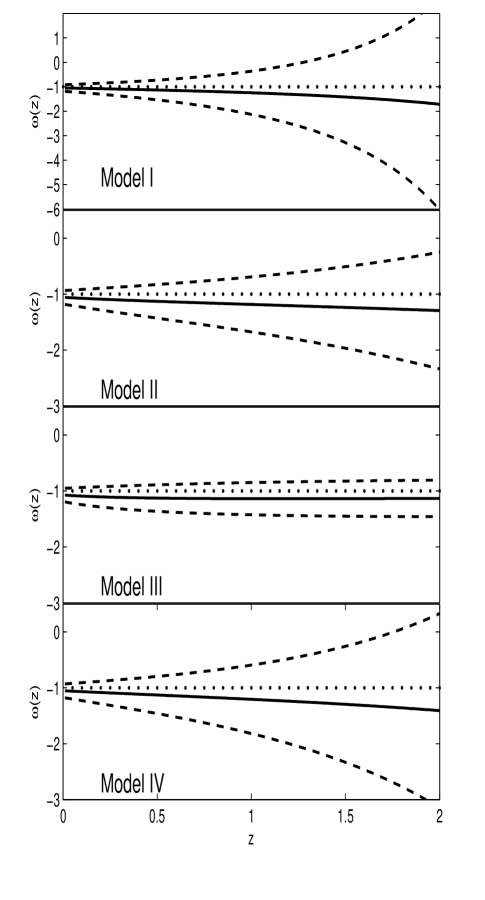
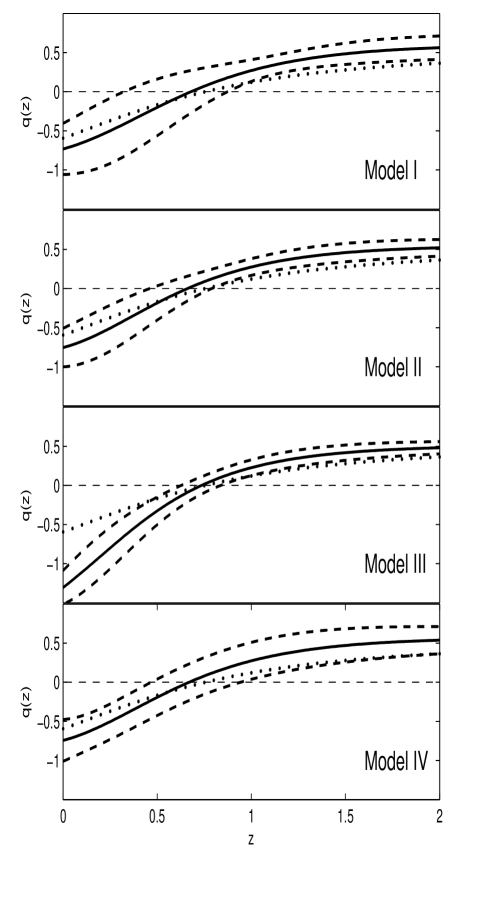
In the right pannel of Fig.5, we plot $w(z)$ of the four jerk models. The best-fit results show $\omega(z)<-1$ in the past, and the departure from -1 enlarges as the redshift $z$ increases. More importantly, the current value $\omega_{0}$ is not strict -1 but a little smaller. This does not contradict with $j(z=0)=-1$ in our calculation since both $j$ and $\omega$ are not constant. It is different from the previous work j..Blandford where a constant $\omega$ is assumed. Taking into account the uncertainty, the $\Lambda$CDM model can be well accommodated in the 1$\sigma$ errors.

III.4 The deceleration factor $q(z)$ and $Om(z)$ diagnostic

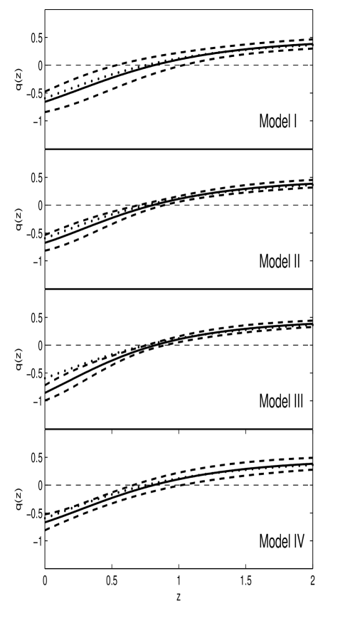
As a further step in tracing the dynamic of the jerk parameterizations, we also calculate the deceleration factor $q(z)$ as Eq.(3) shows. Our results are presented in Fig.6. Since the SNe data sample supports the standard $\Lambda$CDM model, we do not plot its curve and $1\sigma$ errors and only plot the ones of OHD. We use $q(z)$ of the $\Lambda$CDM to represent the SNe results. We find that OHD observations also show an accelerated expansion of the universe in our jerk parameterizations. Despite the bad constraint of the parameters, this phenomenon is proved at high confidence level. One may attribute the reason of the accelerated expansion to the nearly zero value of $j_{1}$ because $j_{1}=0$ leads to $j=-1$ and returns to $\Lambda$CDM model. However, this should be caused by the value of $C_{1}$ in the jerk parameterizations, because a matter-dominated universe (no accelerated expansion) also has $j=-1$ as we discussed in the preceding section.

In addition, $q(z)$ of Model III in Fig.6 behaves differently from other models. The current value $q(z=0)$ is not consistent with $\Lambda$CDM model which can be seen as a deviation at certain extent (even the addition of H_2.3 does not change this). This is not unexpected as seen in Fig.4, the reconstruction of $j(z)$ in Model III. The slope of the best-fit curve at $z=0$ is the largest in Model III which shows a remarkable deviation from $j(z)=-1$ among these models. But we have to say this results are obtained by the use of OHD sample with the first $H_{0}$ prior. When the second prior is used, the deviation disappeared. This is because the constraints are affected at some extent by the choice of prior OHD..Farooq .

Another important epoch of the evolution of the universe is the transition redshift $z_{t}$ when the universe began to expand with an acceleration from the cosmic deceleration phase OHD..Busca ; transition..Lima ; transition..Farooq1 ; transition..Farooq2 . Their works studied the possibility of using the transition redshift as a potential cosmic variable. Except that, their results also show the prediction as the standard $\Lambda$CDM indicates. In the present work, the results obtained from OHD in Fig.6 show that $0.4<z_{t}<1$ for the four jerk parameterizations. This is consistent with the previous works but the uncertainty is obvious j..model2..2 . The addition of H_2.3 improves this estimation as expected, and the consistency between the jerk models may lead us to believe that the transition redshift is not an artifact of the parameterizations.

In our reconstruction, the second term in Eq.(11) can be treated as a perturbation from the standard $\Lambda$CDM model and $j_{1}$ is a measurement of its magnitude. In addition, $j_{1}$ works differently in the four parameterizations. This can be found from the results of $H(z)$, $\omega(z)$ and $q(z)$. Although the calculations show that the different parameterizations have consistent results with each other, it is still of some necessity to find the influence of different functions in choosing $f(z)$ in Eq.(11).

As we know, except for the statefinder diagnostic, another common tool in distinguishing dark energy models is the $Om(z)$ diagnostic which is defined as Om..Sahni

$$Om(z)=\frac{E^{2}(z)-1}{(1+z)^{3}-1}.$$ (39)

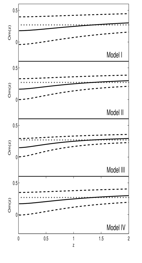
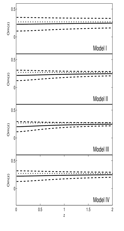
Apparently, $Om(z)=\Omega_{m0}$ for $\Lambda$CDM model, therefore this function is useful and powerful in distinguishing $\Lambda$CDM from other dark energy models. Additionally, since $Om(z)$ relies only on the knowledge of Hubble parameter or equivalently, the expansion factor, the errors in the reconstruction of $Om$ are bound to be small.

On the other hand, since $Om(z)=\Omega_{m0}$ which is the fraction of the matter term in the $\Lambda$CDM model, one may conjecture that the deviation of $Om(z)$ from a constant value $\Omega_{m0}$ in certain dark energy models can represent a perturbation that comes from the effect rather than the matter.

The reconstruction results of $Om(z)$ are presented in Fig.7. The SNe constraint results are just represented by the standard $\Lambda$CDM curve and the $1\sigma$ error is neglected. We can find that the $\Lambda$CDM model can be well accommodated by OHD and OHD+H_2.3 samples, but the best-fit values favor a smaller matter proportion in the low redshift range. Except that, the reconstructed evolution curves of all the four jerk models change little in the redshift range $0<z<2$, especially for the OHD+H_2.3 one. This is caused by the relatively small value of $j_{1}$ and this can be seen as a proof of treating the $j_{1}$ term in Eq.(11) as a perturbation.

Figure 6: The reconstruction of the deceleration factor. The solid lines represent the best-fit curves, while the dashed lines stand for the $1\sigma$ error. $Left$: OHD; $Right$: OHD+H_2.3. The dotted lines stand for the spatially flat $\Lambda$CDM model with $\Omega_{m0}=0.27$ CMB..Komatsu and the horizonal thin dashed lines represent $q=0$.

Figure 7: The reconstruction of the $Om(z)$ diagnostic. The solid lines represent the best-fit curves, while the dashed lines stand for the $1\sigma$ error. $Left$: OHD; $Right$: OHD+H_2.3. The dotted lines stand for the spatially flat $\Lambda$CDM model with $\Omega_{m0}=0.27$.

III.5 The joint constraints

Figure 8: The joint constraints for Model I. $Left$: the OHD with prior of $H_{0}=74.3\pm 2.1$ km s^-1 Mpc^-1 and SNe data with (solid) and without (dotted) systematic errors. $Right$: the OHD with prior of $H_{0}=68\pm 2.8$ km s^-1 Mpc^-1 and SNe data with (solid) and without (dotted) systematic errors. The thin and thick circles belong to dotted and solid contours respectively.

Figure 9: The same as FIG.8 but for Model II.

Figure 10: The same as FIG.8 but for Model III.

Figure 11: The same as FIG.8 but for Model IV.

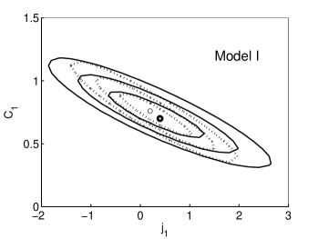
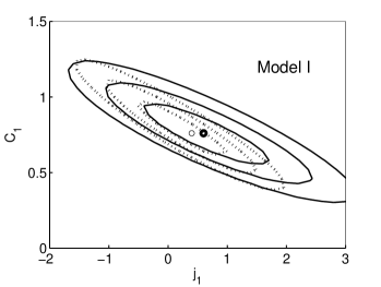
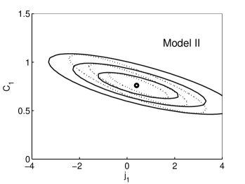
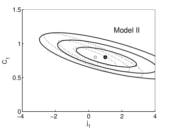
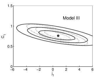
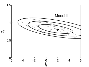
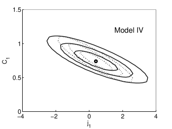
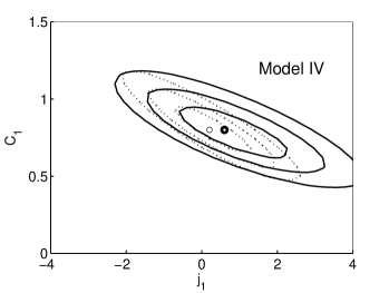
From the previous results, we can see that the SNe and OHD samples give similar constraints on the jerk parameterizations models. Therefore one may expect that the joint constraint of these data could provide tighter constraints. This will give more accurate values of the cosmological parameters and help to discriminate different cosmological models. Our results of the joint constraints are presented in FIG.8 to FIG.11 and TABLE.4 where different combinations of the data samples SNe (with and without systematic errors) and OHD (two choices of the prior of $H_{0}$) are considered. The best-fit values of the parameters are confirmed by minimizing

$$\chi^{2}=\chi_{SNe}^{2}+\chi_{OHD}^{2}.$$ (40)

And the confidence regions are found by the same method as the single constraints.

From the values of FoM, we can see that the joint data improve the constraints significantly. And the best constraint comes from SNe without considering systematic errors plus OHD+H_2.3 with the prior of $H_{0}=74.3\pm 2.1$ km s^-1 Mpc^-1. From the confidence regions, we can conclude that the second prior of $H_{0}$ give worse constraints than the first one. However, it also favors a larger value of $j_{1}$.

The joint constraints give consistent results of the parameter $C_{1}$ and their uncertainties are also sufficiently small. Together with the fact of small value of $j_{1}$, this shows the proportion of the matter in the universe.

	data	$j_{1}$	$C_{1}$	$\chi_{\text{min}}^{2}$	FoM
Model I	SNea+OHD+H2.3($H_{0}^{\prime}$)	$0.20\pm 0.56$	$0.76\pm 0.13$	$584.82$	47.8868
Model I	SNeb+OHD+H2.3($H_{0}^{\prime}$)	$0.40\pm 0.59$	$0.70\pm 0.10$	$569.16$	26.2562
Model I	SNea+OHD+H2.3($H_{0}$)	$0.40\pm 0.39$	$0.76\pm 0.09$	$582.99$	42.2382
Model I	SNeb+OHD+H2.3($H_{0}$)	$0.60\pm 0.73$	$0.76\pm 0.14$	$566.41$	21.3222
Model II	SNea+OHD+H2.3($H_{0}^{\prime}$)	$0.40\pm 0.87$	$0.76\pm 0.09$	$584.95$	27.5121
Model II	SNeb+OHD+H2.3($H_{0}^{\prime}$)	$0.40\pm 1.14$	$0.76\pm 0.09$	$569.18$	15.0537
Model II	SNea+OHD+H2.3($H_{0}$)	$0.40\pm 0.81$	$0.80\pm 0.08$	$582.88$	24.7434
Model II	SNeb+OHD+H2.3($H_{0}$)	$1.00\pm 1.25$	$0.80\pm 0.10$	$566.50$	12.1524
Model III	SNea+OHD+H2.3($H_{0}^{\prime}$)	$0.80\pm 1.27$	$0.76\pm 0.07$	$584.91$	17.1361
Model III	SNeb+OHD+H2.3($H_{0}^{\prime}$)	$0.80\pm 1.69$	$0.76\pm 0.07$	$569.25$	9.2012
Model III	SNea+OHD+H2.3($H_{0}$)	$0.80\pm 1.19$	$0.80\pm 0.07$	$582.96$	15.3857
Model III	SNeb+OHD+H2.3($H_{0}$)	$2.00\pm 1.74$	$0.80\pm 0.07$	$566.64$	7.3906
Model IV	SNea+OHD+H2.3($H_{0}^{\prime}$)	$0.40\pm 0.64$	$0.74\pm 0.08$	$584.81$	36.1403
Model IV	SNeb+OHD+H2.3($H_{0}^{\prime}$)	$0.40\pm 0.87$	$0.74\pm 0.09$	$569.15$	19.6640
Model IV	SNea+OHD+H2.3($H_{0}$)	$0.20\pm 0.73$	$0.80\pm 0.09$	$582.94$	31.9332
Model IV	SNeb+OHD+H2.3($H_{0}$)	$0.60\pm 1.10$	$0.80\pm 0.12$	$566.52$	15.6984

Table 4: The constraint results of the parameters, including the best-fit values with $1\sigma$ errors of the parameters and the FoM of four jerk parameterizations. (The subscripts ”$a$”,”$b$” and prime have the same meanings as TABLE.1 and TABLE.2).

IV discussions and conclusion

In this paper, we study the property of the cosmological jerk parameter in detail. Just within the assumption of a homogeneous and isotropic universe without any introduction of the underlying gravitational theory and energy components, we propose several various kinds of reconstruction of jerk parameter and perform a kinematic analysis and constraint by the SNe and OHD samples.

Our constraining results show that the standard $\Lambda$CDM model can be well accommodated by the SNe and OHD observations. In other words, the $\Lambda$CDM model can be well supported by the evolution of the scale factor up to its third time derivative. Especially, the constraint of SNe data gives a nearly zero value of the parameter $j_{1}$ which is a measurement of the deviation of $j(z)$ from the $\Lambda$CDM model. Once the constraint uncertainties are taken into account, the OHD can give similar results. This is consistent with the previous studies that OHD can play the same role as SNe in constraining cosmological models.

As pointed out in Sec.II.1, the parameterizations of jerk in our work have $j=-1$ at $z=0$. Although the previous works did not show the current universe is strictly the $\Lambda$CDM onej..model2..1 ; j..model2..2 ; j..Rapetti , the concordance $\Lambda$CDM paradigm is also strongly supported j..Rapetti . Moreover, the real value of $j$ at $z=0$ should be directly obtained by the current or at least, the low-redshift observations. However, the low-redshift research is far from comprehensive or efficient enough. For example, the equation of state of the dark energy is allowable and theoretically possible to have arbitrarily large fluctuations at ultra-low redshifts eos..Mortonson . This may increase the uncertainties of the measurements at low redshift. And thus the study of the low redshift cosmology is necessary and of great importance. Except that, There also appears to be some tension between low $z$ and high $z$ data tension..Shafieloo ; tension..Wei . These facts make the confirmation of the current value of $j$ difficult. Thus compared with this potential uncertainty, one possible way is to adopt the simplest model, the $\Lambda$CDM model and ignore the chaotic knowledge.

In order to obtain more information of our reconstruction, we also calculated the Hubble parameter $H(z)$, equation of state $\omega$, deceleration factor $q(z)$ and $Om(z)$ diagnostic of the jerk models. The effect of the addition of H_2.3 is significant in the $\chi^{2}$ constraint which can be seen from Fig.5. Also, the equation of state $\omega<-1$ in the redshift range $0<z<2$ shows a phantom-like universe but the evidence is not strong. The reconstruction of $q(z)$ indicate a current accelerated expansion phase following a matter-dominated phase. This is consistent with the great discovery of Type Ia SNe SNe..Riess ; SNe..Perlmutter . Moreover, we employ the $Om(z)$ diagnostic in our calculation. This kind of function can not only behave as a diagnostic to distinguish different dark energy models from $\Lambda$CDM model. Moreover, We conjecture that it is also useful in studying the kinematic models. Because this kind of models is often obtained mathematically rather than physically, the meanings of the parameters rising from the solution process are hard to handle. From this point of view, $Om$ can be used as a “matter generator” or the “effective” matter term in this kind of cosmological models. Our results show that OHD prefers a smaller value of $Om$ at $z=0$. Additionally, the change of $Om(z)$ in the past was not significant. In other words, $Om(z)$ evolves like a constant. This can be seen as a positive proof of regarding the $j_{1}$ term in the $j(z)$ parameterizations as a perturbation.

In this work, we use two kinds of observational data: Type Ia Supernovae and Hubble parameter. The comparisons between them in constraining cosmological models have been studied for several years. Because of the large size of the data sample and relatively clear systematic errors, SNe always provides more efficient constraint than OHD. However, when the systematic errors of the measurements are taken into account, the constraints from SNe become worse than OHD and this can be seen in our jerk results. Moreover, the latest development in the measurement of Hubble parameter gives us the possibility that the data sample with smaller size also has the power to constrain dark energy models effectively even better than SNe OHD..Farooq2 . Therefore, it is anticipated that the future high-z, high-accuracy $H(z)$ determinations will provide more important contributions in cosmological researches OHD..ZhangT .

In our analysis, the joint constraints are also achieved. As expected, the joint constraints can sufficiently improve the constraining results. And the different combinations of the data samples also give us the information that the parameter $C_{1}$ is confirmed in a high precision.

Additionally, the relationships of SNe and OHD in constraining jerk model should be noticed. As we know, the measurement of SNe comes from the distance modulus, while OHD comes from the ages of passively evolving galaxies, BAO measurement and so forth. If we regard the SNe observations as the distance measurement, OHD should be related to the velocity measurement which is a time derivative of the distance. Thus the information of acceleration or higher order derivative (such as jerk, snap etc.) can be obtained from distance or velocity measurement respectively. One question is that what is the difference when we use distance and velocity respectively to study the acceleration or jerk? An important issue is the error propagation. The number of derivative from distance to acceleration or higher-order variables is bigger than that from velocity to them. So this may increase the uncertainty in estimating the acceleration and jerk. From this point of view, the OHD should be a better tool in studying the evolution of the universe, especially when we hope to find more accurate and subtle information of the universe since this kind of information can be well carried by the higher order derivative of the scale factor.

V acknowledgement

We are very grateful to the anonymous referee for his valuable comments and suggestions that greatly improve this paper. The authors would like to thank W-B Liu for helpful discussions and suggestions. This work is supported by the Ministry of Science and Technology National Basic Science program (project 973) under grant No. 2012CB821804, the National Natural Science Foundation of China (Grant Nos. 11173006, 10875012, 11235003 and 11365008), the Fundamental Research Funds for the Central Universities and the Natural Science Fund of Education department of Hubei Province (Grant No. Q20131901).

References

- (1) A. G. Riess, A. V. Filippenko, P. Challis et al., Astron J., 116, 1009 (1998)
- (2) M. Hicken, W. M. Wood-Vasey, S. Blondin et al., Astrophys J., 700, 1097 (2009)
- (3) S. Perlmutter et al., Astrophys. J., 517, 565 (1999)
- (4) D. N. Spergel, R. Bean, O. Doré et al., Astrophys. J. S., 170, 377 (2007)
- (5) E. Komatsu, K. M. Smith, J. Dunkley et al., Astrophys. J. S., 192, 18 (2011)
- (6) D. J. Eisenstein, I. Zehavi, D. W. Hogg et al., Astrophys. J., 633, 560 (2005)
- (7) W. J. Percival, B. A. Reid, D. J. Eisenstein et al., Mon. Not. Roy. Astron. Soc., 401, 2148 (2010)
- (8) Weinberg, D. H. et al., eprint, arXiv: 1201.2434
- (9) S. Tsujikawa, eprint, arXiv: 1004.1493
- (10) J. Sola, eprint, arXiv: 1306.1527
- (11) M. Li et al., Commun. Theor. Phys. 56, 525 (2011)
- (12) S. Capozziello and M. Laurentis, Phys. Rept., 509, 167 (2011)
- (13) M. Trodden, eprint, arXiv: 1212.6399
- (14) H. Jassal et al., Mon. Not. Roy. Astron.S oc. 405, 2639 (2010)
- (15) K. Wilson et al., Mod. Phys. Lett. A, 21 2197 (2006)
- (16) T. Davis et al., Astrophys. J., 666, 716 (2007)
- (17) S. Allen et al., Mon. Not. Roy. Astron. Soc., 383, 879 (2008)
- (18) S.Weinberg, eprint, arXiv: astro-ph/0005265
- (19) A. Vilenkin, eprint, arXiv: hep-th/0106083
- (20) J. Garriga, M. Livio and A. Vilenkin, Phys. Rev. D, 61, 023503 (2000)
- (21) G. Caldera-Cabral, R. Maartens and L. A. Urena-Lopez, Phys. Rev. D, 79, 063518 (2009)
- (22) J. V. Cunha, Phys. Rev. D, 79, 047301 (2009)
- (23) J. -M. Virey, et al., Phys. Rev. D, 72, 061302 (2005)
- (24) C. Stephan-Otto, Phys. Rev. D, 74, 023507 (2006)
- (25) Z. L. Yi and T. J. Zhang, Mod. Phys. Lett. A, 22, 41 (2007)
- (26) D. Huterer and G. Starkman, Phys. Rev. Lett., 90, 031301 (2003)
- (27) C. Shapiro and M. S. Turner, Astrophys. J., 649, 563 (2006)
- (28) S. del Campo et al., Phys. Rev. D, 86, 083509 (2012)
- (29) R. D. Blandford et al., eprint, arXiv: astro-ph/0408279
- (30) M. Visser, Class. Quant. Grav., 21, 2603 (2004)
- (31) Ø. Elgarøy and T. Multamäki, J. C. A. P., 09, 002 (2006)
- (32) A. C. C. Guimarães et al., J. C. A. P., 10, 010 (2009)
- (33) M. P. Dabrowski, Phys. Lett. B, 625, 184 (2005)
- (34) M. P. Dabrowski and A. Balcerzak, eprint, arXiv:gr-qc/0701056
- (35) V. Sahni et al., J. E. T. P. Lett., 77, 201 (2003)
- (36) U. Alam et al., Mon. Not. Roy. Astron. Soc., 344, 1057 (2003)
- (37) S. Capozziello et al., Phys. Rev. D, 78, 063504 (2008)
- (38) M. Dunajski and G. Gibbons, Class. Quant. Grav., 25, 235012 (2008)
- (39) N. J. Poplawski, Phys. Lett. B, 640, 135 (2006)
- (40) L. Xu and Y. Wang, Phys. Lett. B, 702, 114 (2011)
- (41) L. Xu, W. Li and J. Lu, J. C. A. P., 0907, 031 (2009)
- (42) J. Lu et al., Phys. Lett. B, 699, 246 (2011)
- (43) D. Rapetti et al., Mon. Not. Roy. Astron. Soc., 375, 1510 (2007)
- (44) A. G. Riess et al., Astrophys. J., 607, 665 (2004)
- (45) I. Maor, R. Brustein and P. Steinhardt, Phys. Rev. Lett., 86, 6 (2001)
- (46) S. Basilakos, D. Polarski and J. Sola, Phys. Rev. D, 86, 043010 (2012)
- (47) N. Suzuki et al., Astrophys. J., 746, 85 (2012)
- (48) O. Farooq, D. Mania and B. Ratra, eprint, arXiv: 1211.4253
- (49) Y. Chen, and B. Ratra, Phys. Lett. B, 703, 406 (2011)
- (50) E. Mueller, R. Bean, S. Watson, eprint, arXiv: 1209.2706
- (51) J. Lu et al., J. C. A. P., 1003, 031 (2010)
- (52) J. Grande et al., J. C. A. P., 1108, 007 (2011)
- (53) S. Basilakos, M. Plionis and J. Sola, Phys. Rev. D, 80, 083511 (2009)
- (54) H. Zhang and Z. Zhu, J. C. A. P., 0803, 007 (2008)
- (55) X. Duan, Y. Li and C. Gao, eprint, arXiv: 1111.3423
- (56) K. Liao et al., Phys. Lett. B, 710, 17 (2012)
- (57) S. Cao, N. Liang and Z. Zhu, Mon. Not. Roy. Astron. Soc.,416, 1099 (2011)
- (58) S. Cao, N. Liang and Z. Zhu, eprint, arXiv: 1105.6274
- (59) W. Godłowski and M. Szydłowski, Phys. Lett. B, 623, 10 (2005)
- (60) R. Lazkoz and E. Majerotto, J. C. A. P., 0707, 015 (2007)
- (61) H. Wei and S. Zhang, Phys. Lett. B, 654 139 (2007)
- (62) P. Wu and H. Yu, J.C.A.P. 0703, 015 (2007)
- (63) A. Kurek and M. Szydlowski, Astrophys. J., 675 1 (2008)
- (64) X. Zhang, Phys. Rev. D, 79, 103509 (2009)
- (65) C. Ma, T. Zhang, Astrophys. J., 730 74 (2011)
- (66) T. Zhang, C.Ma and T. Lan, Advances in Astronomy, 184284 (2010)
- (67) Z. Zhai, H. Wan and T. Zhang, Phys. Lett.B, 689, 8 (2010)
- (68) H. Lin et al., Mod. Phys. Lett. A, 22, 1699 (2009)
- (69) R. Cai and A. Wang, J. C. A. P., 0503, 002
- (70) M. Chevallier and D. Polarski, Int. J. Mod. Phys. D, 10, 213 (2001)
- (71) E. V. Linder, Phys. Rev. Lett., 90, 091301 (2003)
- (72) H. Jassal, J. Bagla and T. Padmanabhan, Mon. Not. Roy. Astron. Soc., 356, L11 (2005)
- (73) S. Nesseris and L. Perivolarropoulos, Phys. Rev. D, 72, 123519 (2005)
- (74) R. Jimenez, A. Loeb, Astrophys. J., 573, 37 (2002)
- (75) R. Jimenez, L. Verde, T. Treu and D. Stern, Astrophys. J., 593, 622 (2003)
- (76) J. Simon, L. Verde and R. Jimenez, Phys. Rev. D, 71, 123001 (2005)
- (77) D. Stern, R. Jimenez, L. Verde, M. Kamionkowski and S. A. Stanford, J.C.A.P., 02, 008 (2010)
- (78) E. Gaztañaga, E. Cabré and L. Hui, Mon. Not. Roy. Astron. Soc., 399, 1663 (2009)
- (79) M. Moresco et al., J. C. A. P., 1208, 006 (2012)
- (80) W. Freedman et al., Astrophys. J., 758, 24 (2012)
- (81) G. Chen and B. Ratra, eprint, arXiv: 1105.5206
- (82) Planck Collaboration, eprint, arXiv: 1303.5076
- (83) N. Busca et al., eprint, arXiv: 1211.2616
- (84) A. Albrecht et al., eprint, arXiv: astro-ph/0609591.
- (85) D. Huterer and M. S. Turner, Phys. Rev. D, 64, 123527 (2001)
- (86) M. Mortonson, W. Hu, and D. Huterer, Phys. Rev. D, 82, 063004 (2010).
- (87) E. Ruiz et al., Phys. Rev. D, 86, 103004 (2012)
- (88) Coe, D., eprint, arXiv: 0906.4123
- (89) O. Farooq and B. Ratra, eprint, arXiv: 1212.4264
- (90) A. Astashenok et al., Phys. Lett. B, 709, 396 (2012)
- (91) P. Frampton, K. Ludwick and R. Scherrer, Phys. Rev. D, 84, 063003 (2011)
- (92) P. Frampton, K. Ludwick and R. Scherrer, Phys. Rev. D, 85, 083001 (2012)
- (93) J. A. S. Lima et al., eprint, arXiv: 1205.4688
- (94) O. Farooq and B. Ratra, eprint, arXiv: 1301.5243
- (95) O. Farooq et al., eprint, arXiv: 1305.1957
- (96) V. Sahni, A. Shafieloo and A. A. Starobinsky, Phys. Rev. D, 78, 103502 (2008)
- (97) M. J. Mortonson, W. Hu and D. Huterer, Phys. Rev. D, 80, 067301 (2009)
- (98) A. Shafieloo, V. Sahni and A. Starobinsky, Phys. Rev. D, 80, 101301 (2009)
- (99) H. Wei, Phys. Lett. B, 687, 286 (2010)