Emergent Exclusion Statistics of Fibonacci Anyons in 2D Topological Phases

Abstract

We demonstrate how the generalized Pauli exclusion principle emerges for quasiparticle excitations in 2d topological phases. As an example, we examine the Levin-Wen model with the Fibonacci data (specified in the text), and construct the number operator for fluxons living on plaquettes. By numerically counting the many-body states with fluxon number fixed, the matrix of exclusion statistics parameters is identified and is shown to depend on the spatial topology (sphere or torus) of the system. Our work reveals the structure of the (many-body) Hilbert space and some general features of thermodynamics for quasiparticle excitations in topological matter.

1. Introduction

By now it is well-known that (quasi-)particles in strongly entangled many-body systems may exhibit exotic quantum statistics, other than the familiar Bose-Einstein and Fermi-Dirac ones. In addition to the anyonic or exchange statistics Wilczeck in two dimensional systems, statistical weight of many-body quantum states may also obey new combinatoric counting rules Wu2 following a generalized Pauli exclusion principle Haldane , in which the number of available single-particle states, when adding one more quasi-particle into the system, linearly depends on the number of existing quasi-particles. A typical new feature is mutual exclusion between different species, resulting in a matrix of statistical parameters Haldane and leading to unusual thermodynamics for ideal gases with only statistical interactionsWu2 ; footnote1 . (For a review see, e.g., ref. Wu1994, .)

More precisely, following ref. Wu2, , in the case with only one species of quasi-particles, the number of $N$-particle states is assumed to be given by the binomial coefficient:

$$W_{G,N}=\binom{G_{\text{eff}}+(N-1)}{N},$$ (1)

with $G_{\text{eff}}=G-\alpha(N-1)$ being the number of available single-particle states, while $G$ is the number of single-particle states when $N=1$. Then $\alpha=0$ corresponds to bosons and $\alpha=1$ fermions; other values of $\alpha$ gives rise to exotic exclusion statistics. Similarly, in the multi-species case, the number of many-particle states is assumed to be given by ($a,b=1,\dots,m$ labeling species)

$$W_{\{G_{a},N_{a}\}}=\prod_{a}\binom{G_{a}+N_{a}-1-\sum_{b=1}^{m}\alpha_{ab}\left(N_{b}-\delta_{ab}\right)}{N_{a}}.$$ (2)

Here coefficients $\alpha_{ab}$ form the (mutual) statistics matrix.

It has been shown WuBernard that the Thermodynamic Ansatz YangYang for one-dimensional solvable many-particle models is actually a special case of the exotic exclusion statistics. (See also refs. Ha, ; Kohmoto, .) It has been also numerically verified that quasi-particle excitations in the fractional quantum Hall (FQH) systems indeed obey Zhang eq. (1), or eq. (2) allowing mutual exclusion between different speciesSuWuYang . Moreover either the Haldane or Jain hierarchy in the FQH effect can be theoretically understood from the exclusion statistics of quasiparticlesWu1994 ; YuYue .

Recently there has been revived interest in the study of quasiparticle statistics in 2d topological states of matter (including FQH systems), because of the possibility of using their braiding to do (fault tolerant) topological quantum computation (TQC) Kitaev ; Wang . In order to know better about the error of TQC at finite temperature, it is needed to understand better how exclusion statistics of quasi-particles emerges in 2d topological matter, which governs the thermodynamics of the system.

In this letter, we carry out the many-body state counting in an exactly solvable discrete model, i.e., the Levin-Wen modelLW (with a special set of data), that describes a 2d topological quantum fluidGil0906 of Fibonacci anyonsSB , with doubled Fibonacci anyons as fluxon excitations living on plaquettes. The Fibonacci anyons are the simplest non-abelian anyons. They occur as quasiparticles in the $k=3$ Read-Rezayi stateRR in an FQH state with filling fraction $\nu=\frac{12}{5}$, and can be used for universal topological quantum computationWang . (Recently, it is proposedLK that the physics of interacting Fibonacci anyons may be studied in a Rydberg lattice gas.)

In this Letter, we first construct the number operator for fluxons in the model, which helps us identify the states with localized excitations. Then we numerically count the (many-body) states with fluxon-number $N$ fixed, from $N=1$ up to $N=7$, for the system on a sphere and torus, respectively. The results exhibit a pattern closely related to the Fibonacci numbers, which in turn is put in the form of eq. (2), thus determining a topology-dependent statistics parameter matrix. Our work reveals that exotic exclusion emerges among quasiparticles due to interplay between various “hidden” degrees of freedom (d.o.f.) in addition to fluxon locations. These “hidden” d.o.f. are very similar to the pseudo-species, previously introduced in the literature on conformal field theoryGS , which do not contribute to energy but contribute to state-counting in accordance with an exclusion statistics parameter matrix. Finally, we briefly discuss the thermodynamics of the system.

2. The model

We consider a discrete model for a “spin” system on a trivalent graph on a closed surface, e.g. a sphere or torus. We adopt a simplified formulation of the Levin-Wen model LW , with the Fibonacci data (e.g., see ref. Wang, ) given as follows: Each link is assigned a “spin”-type labeled by $j$ and configurations of the labels on all links form an orthonormal basis in the Hilbert space. The key input of the Fibonacci data is that the “spin”-type index $j$ takes only two values $j=0,1$, and they satisfy an algebra (called the Fibonacci algebra), which describes how to fuse two “spin”-types through the branching rules:

$$0\otimes j=j\otimes 0=j,1\otimes 1=0\oplus 1.$$ (3)

These rules are similar to those for the (direct sum) decomposition of (tensor) products of irreducible representations of a group, with $j=0$ playing the role of the unit element for the (tensor) product. (It is conjectured that the Levin-Wen model describes a class of doubled (time-reversal invariant) topological phases Freedman .)

The Hamiltonian of the model is of the form

$$\hat{H}=U\sum_{v}(1-\hat{Q}_{v})+\epsilon\sum_{p}(1-\hat{B}_{p}),\quad\hat{B}_{p}=\frac{1}{D}\sum_{s=0,1}d_{s}\hat{B}_{p}^{s}.$$ (4)

The two summations here run over all vertices $v$ and plaquettes $p$, respectively. For $\hat{B}_{p}$, the summation runs over the “spin”-type $s=0,1$, and $d_{0}=1$,$d_{1}=\phi\equiv{(\sqrt{5}+1)/2}$, and $D=1+\phi^{2}$. $U$ and $\epsilon$ are positive constants. The explicit form of the operators $\hat{Q}_{v}$ and $\hat{B}_{p}^{s}$ are given in the supplemental materialsuppl . (By adding more competing interactions, ref. Vidal has used this model to discuss topological phase transitions in the Fibonacci anyon liquid. Here we restrict to the original Levin-Wen model and discuss emergent exclusion statistics for quasi-excitations.)

A notable property of the model is that by construction, $\hat{Q}_{v}$ and $\hat{B}_{p}$ are mutually commuting projection operators: $[\hat{Q}_{v},\hat{B}_{p}]=0$, $\hat{Q}_{v}\hat{Q}_{v^{\prime}}=\delta_{vv^{\prime}}\hat{Q}_{v}$ and $\hat{B}_{p}\hat{B}_{p^{\prime}}=\delta_{pp^{\prime}}\hat{B}_{p}$. Thus the Hamiltonian is exactly solvable. The energy eigenstates are the simultaneous eigenvectors of these projections $\hat{Q}_{v}$ and $\hat{B}_{p}$. The ground states are those $|{\Phi}\rangle$ that satisfy $\hat{Q}_{v}|{\Phi}\rangle=|{\Phi}\rangle=\hat{B}_{p}|{\Phi}\rangle$, for all $v$ and $p$. Using the method developed in ref. GSD, , one can compute ground state degeneracy: $\text{GSD}=1$ on sphere and $\text{GSD}=4$ on torus.

The quasiparticle excitations are the states with zero eigenvalue of $\hat{Q}_{v^{\prime}}$ for some $v^{\prime}$ and/or of $\hat{B}_{p^{\prime}}$ for some $p^{\prime}$. $\hat{B}_{p^{\prime}}|{\Psi}\rangle=0$). In this letter we restrict ourselves to study the so-called fluxons, satisfying $\hat{Q}_{v}=1$ for all $v$, $\hat{B}_{p^{\prime}}=0$ for a specified set of $p^{\prime}$ (where fluxons live), and $\hat{B}_{p}=1$ for all other $p$. (See Fig. 1.)

Figure 1: A configuration in the subspace with only fluxons allowed, with solid lines for $j=1$ and dotted lines $j=0$. Open strings (with only single solid line at some vertex) are forbidden by $\delta_{001}=0$.

3. Number operator of fluxons

A crucial property of the model is that ${\hat{B}_{p}^{s}}$ defined above form an abelian algebraLW :

$$\hat{B}_{p}^{r}\hat{B}_{p}^{s}=\sum_{t=0,1}\delta_{rst}\hat{B}_{p}^{t},$$ (5)

Here $\delta_{ijk}=\delta_{jki}=\delta_{jik}$ is given by $\delta_{000}=\delta_{011}=\delta_{111}=1$, arising from the branching rules (3). From the generators we construct the operators ($i=0,1$):

$$\hat{n}_{p}^{i}=\sum_{j=0,1}S_{i0}S_{ij}\hat{B}_{p}^{j},$$ (6)

where $S$ is the modular matrix given by

$$S=\frac{1}{\sqrt{D}}\left(\begin{array}[]{cc}1&\phi\\ \phi&-1\end{array}\right),$$ (7)

with $S_{ij}$ for fixed $i$ being a one-dimensional representation of the algebra (5). One can check that $\hat{n}_{p}^{i}$ ($i=0,1$) form a complete set of orthonormal projections:

$$\hat{n}_{p}^{i}\hat{n}_{p}^{k}=\delta_{ik}\hat{n}_{p}^{k},\quad\hat{n}_{p}^{0}+\hat{n}_{p}^{1}=\mathbf{1}.$$ (8)

There is a fluxon at $p$ in a state $|{\Psi}\rangle$, if $\hat{n}_{p}^{1}|{\Psi}\rangle=|{\Psi}\rangle$. A ground state $|{\Phi}\rangle$ contains no fluxon because $\hat{n}_{p}^{0}=\hat{B}_{p}$. Hence the model has only one type of fluxons, and there is no state with two fluxons living at the same plaquette $p$. This seems to indicate that the flux in this model should be a fermion (or a hard boson). In the following we will present a study of many-fluxon state counting in this model, which reveals that actually the fluxons in this model obey instead exotic exclusion statistics which was proposed in refs. Haldane, ; Wu2, . (See also the footnotefootnote .)

4. Exclusion statistics on a sphere

Let us count the $N$-fluxon states in the model with $P$ plaquettes on a sphere. Pick up a set of $N$ fixed plaquettes and denote it by $\mathcal{C}=\{p_{1},p_{2},...,p_{N}\}$ ($N<P$). The states with exactly $N$ fluxons occupying the selected plaquettes are those $|{\psi}\rangle$ satisfying

$$\hat{n}_{p}^{j}|{\Psi}\rangle=\delta_{j1}|{\Psi}\rangle,\quad\text{ for }p\in{\mathcal{C}},$$

$$\hat{n}_{p^{\prime}}^{j}|{\Psi}\rangle=\delta_{j0}|{\Psi}\rangle,\quad\text{ for }{p^{\prime}}\notin{\mathcal{C}}.$$ (9)

Thus $\left(\prod_{p\in{\mathcal{C}}}\hat{n}_{p}^{1}\prod_{p^{\prime}\notin{\mathcal{C}}}\hat{n}_{p^{\prime}}^{0}\right)$ is the projector onto the subspace of such states. Tracing this projection computes the total number of the $N$-fluxon states in the configuration $\mathcal{C}$:

$$w_{P,N,\mathcal{C}}=\text{tr}(\prod_{p\in{\mathcal{C}}}\hat{n}_{p}^{1}\prod_{p^{\prime}\notin{\mathcal{C}}}\hat{n}_{p^{\prime}}^{0}).$$ (10)

We numerically compute eq. (10) on random graphs on sphere with $P(\geq 7)$ plaquettes, with the stable result presented in Table 1.

Table 1: State Counting on Sphere

Fluxon number $N$		0	1	2	3	4	5	6	7
State Counting $w_{P,N,\mathcal{C}}$		1	0	1	1	4	9	25	64

The pattern of the $N$-dependence is obvious:

$$w_{P,N,\mathcal{C}}=F_{N-1}^{2},$$ (11)

where $F_{n}$ is the Fibonacci number that satisfies the recurrence relation $F_{n}=F_{n-1}+F_{n-2}$ with $F_{1}=F_{2}=1$. Both numerically and analytically we have checked that eq. (11) is independent of the graph, of the total number $P$ of plaquettes, as well as the locations of the $N$ fluxons. The appearance of the squared in eq. (11) is consistent with the conjecture that the LW model describes a doubled topological phases Freedman ; GSD .

Summing over configurations $\mathcal{C}$ (i.e., over possible distributions of N plaquettes in a fixed graph), we get the total number of $N$-fluxon states:

$$W_{P,N}^{\text{sphere}}=\sum_{\mathcal{C}}w_{P,N,\mathcal{C}}=\binom{P}{N}F_{N-1}^{2}.$$ (12)

The first factor counts the ways to distribute $N$ fluxons over $P$ plaquettes. The second factor counts the states of the link d.o.f., which are not unique, given $N$ and $\mathcal{C}$. The independence of $w_{P,N,\mathcal{C}}$ on $P$ and $\mathcal{C}$ implies the degeneracy of the excited states is topological in the sense that it does not depend on the detailed structure of the underlying graph, and not on the relative positions between the fluxons as well. We have numerically check particularly this property (see the supplemental meterial suppl . The origin of this property lies in the topological symmetry of the model under mutations of the underlying graphGSD .

To find the exclusion statistics, we rewrite (12):

$$W_{P,N}^{\text{sphere}}=\binom{P}{N}\sum_{N_{1},N_{2}=0}^{[\frac{1}{2}(N-2)]}\binom{N-N_{1}-2}{N_{1}}\binom{N-N_{2}-2}{N_{2}},$$ (13)

where $[x]$ is the greatest integer less than or equal to $x$.

Now eq. (13) is of the form of eq. (2), by introducing two additional pseudo-species $a=1,2$, which do not contribute to the total energy but are helpful for state-counting. This is similar to what was suggested for state counting in some conformal field theories GS . Including the original fluxon species labeled by $a=0$, from eq. (13) we read the exclusion statistics parameters $\alpha_{ab}$ ($a,b,=0,1,2$):

$$\alpha^{\text{sphere}}=\left(\begin{array}[]{ccc}1&0&0\\ -1&2&0\\ -1&0&2\end{array}\right).$$ (17)

The diagonal $\alpha_{aa}$ is the self-exclusion statistics for species $a$. The $\alpha_{00}=1$ implies the hard-core boson behavior, that takes care of the first combinatoric factor in $\binom{P}{N}$ in eq. (12) and eq. (13). This can be understood with eq. (8).

The pseudo-species provides a way to count states, in the presence of fluxons, of link d.o.f., which are not uniquely determined by the constraints (Emergent Exclusion Statistics of Fibonacci Anyons in 2D Topological Phases). The value $\alpha_{11}=\alpha_{22}=2$ implies that one pseudo-particle makes two single-particle states (or “seats”) unavailable to an additional pseudo-particle. The negative mutual statistics $\alpha_{20}=\alpha_{30}=-1$ tells us that each fluxon present creates one vacant “seat” for each pseudo-species. So the maximum particle number of each pseudo-species is naturally $[(N-1)/2]$. These results help us understand the structure of the (many-body) Hilbert space for excited states of the system, and help derive analytically the state counting formula (13). (A sketch of such a derivation is presented in the supplemental materialsuppl .)

We note that the many-body counting formula eq. (2), proposed in ref. Wu2, , with the statistical matrix (17), exactly reproduces the result, Table 1, of numerical counting for fluxon numbers from $N=0$ to $N=7$. It is remarkable that the counting formula eq. (2) is valid even for very small values of the fluxon number, so we believe it is an exact result, true for all values of $N$, including the thermodynamical limit.

6. Exclusion statistics on a torus

We proceed to consider the model on a torus. The ground state degeneracyGSD is 4 . Thus the system exhibits the global topological d.o.f., and we can study their effects on excited states by counting the pseudo-particle states.

Pick up $N$ plaquettes ($N<P$). The number of states with $N$ fluxons on htese plaquettes is computed numerically as in Table 2.

Table 2: State Counting on Torus

Fluxon number $N$		0	1	2	3	4	5	6
State Counting		$2^{2}$	1	$3^{2}$	$4^{2}$	$7^{2}$	$11^{2}$	$18^{2}$

The pattern of its dependence on $N$ is

$$W_{P,N}^{\text{torus}}=\binom{P}{N}L_{N}^{2},$$ (18)

with $L_{n}$ the Lucas number, a modified version of the Fibonacci number, satisfying the recurrence relation $L_{n}=L_{n-1}+L_{n-2}$ with $L_{1}=1,L_{2}=3$.

We rewrite (18) in terms of binomial coefficients:

$$W_{P,N}^{\text{torus}}= \binom{P}{N}\sum_{N_{1},N_{2}=0,1}\binom{1}{N_{1}}\binom{1}{N_{2}}\times$$

$$\sum_{N_{3},N_{4}=0}^{[\frac{1}{2}(N-2)]}\binom{N-2N_{1}-N_{3}}{N_{3}}\binom{N-2N_{2}-N_{4}}{N_{4}},$$ (19)

and get the exclusion statistics parameters $\alpha_{ab}$ ($a,b=0,1,2,3,4$):

$$\alpha^{\text{torus}}=\left(\begin{array}[]{ccccc}1&0&0&0&0\\ 0&1&0&0&0\\ 0&0&1&0&0\\ -1&2&0&2&0\\ -1&0&2&0&2\end{array}\right),$$ (25)

where we denote by $a=0$ the fluxon species.

Eq. (Emergent Exclusion Statistics of Fibonacci Anyons in 2D Topological Phases) shows that one needs to introduce four pseudo-species $a=1,2,3,4$. The pseudo-species $a=1,2$ are interpreted as the topological d.o.f. on the torus, for the following reasons. The allowed “particle number” $N_{1},N_{2}=0,1$ of these pseudo-species are independent of the number $N$ of fluxons. Particularly when there is no fluxon present, the configurations $N_{1},N_{2}=0,1$ characterize the four-degenerate ground states. Then the pseudo-species $a=3,4$ provide a way to count the states of link d.o.f. given a ground state and fluxon number.

The state counting of excitations on a torus is shown different from that on a sphere. (A state counting formula of different form from ours, which also exhibits the dependence on the spatial topology, is reported in ref. Vidal, , without making connection to exclusion statistics.) Indeed the mutual statistics parameters $\alpha_{31}=\alpha_{42}=2$ imply that the number of states of link d.o.f. $a=3$ ($a=4$) are affected by the topological d.o.f. $a=1$ ($a=2$), respectively. On the other hand, the topological d.o.f. are not affected by the fluxons present and the link d.o.f.. So the degenerate ground states can be used to label the sectors of excitations. We note that in the sector with $N_{1}=N_{2}=1$, the state counting for fluxons is exactly the same as that on sphere.

7. Statistical Thermodynamics

Now we assume that only fluxons can be thermally excited; this is the case when $U>>\epsilon,kT$ in eq. (4). In the thermodynamic limit, the Hilbert space dimension of $N$-fluxon states (occupying $N$ fixed plaquettes) is asymptotically

$$\text{on sphere: }\quad\lim_{N\to\infty}\,F_{N-1}^{2}\sim\phi^{2N-2}/5,$$

$$\text{on torus: }\quad\quad\lim_{N\to\infty}\,L_{N}^{2}\sim\phi^{2N}.$$ (26)

($\phi^{2}$ is called the quantum dimension of the fluxon.) On a torus, for example, the canonical partition function is

$$Z^{\text{torus}}=\sum_{N=0}^{P}\binom{P}{N}L_{N}^{2}e^{-N\epsilon/kT}\sim(\phi^{2}e^{-\epsilon/kT}+1)^{P}.$$ (27)

It can be interpreted as the grand canonical partition function of the many-fluxon system, which behaves like a fermionic system with a temperature-independent fugacity $z$ given by the quantum dimension:

$$z=\phi^{2}.$$ (28)

The fugacity $z$ counts the effective number of states per fluxon located at a plaquette. Note that $z$ is irrational rather than integer. This is a manifestation that the many-fluxon states are highly entangled ones with long-range entanglement. They are superpositions of highly constrained $j$-configurations on the links, obviously not of the form of a direct product of localized fluxon states.

product thermodynamic behavior example, energy of any $N$-fluxon state is equal to with the chemical potential set to zero.

The statistical distribution of the average occupation number of fluxons is obtained from eq. (27):

$$\langle n\rangle=\langle N\rangle/P=\frac{1}{e^{\epsilon/kT}{\phi^{-2}}+1}.$$ (29)

Many useful thermodynamic observables are then computable. The probability for thermal excitations of fluxons that cause errors in topological quantum computation which uses the code based on this model can then be estimated more accurately than before.

Though the model is very simple, we believe that the features revealed in this letter should be quite general for emergent exotic exclusion statistics and thermodynamics for quasiparticle excitations in a wide class of 2d topological phases. Moreover, the knowledge and insights gained in this model for the Hilbert space structure of many-fluxon states may be useful in the future for fault-tolerant quantum computation codes and alogrithms that explore systems in topological phases.

Acknowledgement: YH thanks Department of Physics, Fudan University for warm hospitality he received during a visit in summer 2011 and 2012. YSW was supported in part by US NSF through grant No. PHY-1068558.

Supplementary Material

I Explicit Hamiltonian of the Levin-Wen Model

The operator $\hat{Q}_{v}$ defined at vertex $v$ in the Hamiltonian (4) in the text is

$$\hat{Q}_{v}\left|\begin{matrix}{\leavevmode\hbox to35.93pt{\vbox to28.66pt{\text{[drawing]}}}}\end{matrix}\right\rangle=\delta_{j_{1}j_{2}j_{3}}\left|\begin{matrix}{\leavevmode\hbox to35.93pt{\vbox to28.66pt{\text{[drawing]}}}}\end{matrix}\right\rangle. j_{1} j_{2} j_{3} v j_{1} j_{2} j_{3} v j_{1} j_{2} j_{3} v j_{1} j_{2} j_{3} v$$ (30)

(Only the relevant part of the graph is shown; the rest of the graph is the same on both sides.) Here $\delta_{ijk}=\delta_{jki}=\delta_{jik}$ is given by

$$\delta_{000}=\delta_{011}=\delta_{111}=1,\delta_{001}=0$$ (31)

(called the Fibonacci fusion ruleWang ).

The operator $\hat{B}_{p}^{s}$ defined at plaquette $p$ in the Hamiltonian (4) in the text is

$$\Biggl{\langle}\begin{matrix}{\leavevmode\hbox to56.09pt{\vbox to45.64pt{\text{[drawing]}}}}\end{matrix}\Biggr{|}\hat{B}_{p}^{s}\Biggl{|}\begin{matrix}{\leavevmode\hbox to56.09pt{\vbox to44.94pt{\text{[drawing]}}}}\end{matrix}\Biggr{\rangle} j^{\prime}_{1} j^{\prime}_{2} j^{\prime}_{3} j_{4} j_{5} j_{6} p j_{1} j_{2} j_{3} j_{4} j_{5} j_{6} p$$

$$= v_{j_{1}}v_{j_{2}}v_{j_{3}}v_{j^{\prime}_{1}}v_{j^{\prime}_{2}}v_{j^{\prime}_{3}}G^{j_{5}j_{1}j_{3}}_{sj^{\prime}_{3}j^{\prime}_{1}}G^{j_{4}j_{2}j_{1}}_{sj^{\prime}_{1}j^{\prime}_{2}}G^{j_{6}j_{3}j_{2}}_{sj^{\prime}_{2}j^{\prime}_{3}},$$ (32)

where $v_{j}\equiv{\sqrt{d_{j}}}$. A similar rule applies when the plaquette $p$ is a quadrangle, a pentagon, or a hexagon etc. Note that the matrix is nondiagonal only on the labels of the boundary links (i.e., $j_{1}$, $j_{2}$, and $j_{3}$ on the above graph).

In the Fibonacci data, the non-vanishing $6j$-symbol $G$’s are given by

$$G^{000}_{000}=1,G^{011}_{011}=G^{011}_{111}=1/\phi,$$

$$G^{000}_{111}=1/\sqrt{\phi},G^{111}_{111}=-1/{{\phi}^{2}},$$ (33)

with the (tetrahedral) symmetry:

$$G^{ijm}_{kln}=G^{mij}_{nkl}=G^{klm}_{ijn}=G^{jim}_{lkn}.$$ (34)

One can check that they satisfy the conditions:

$$\text{pentagon id:}\quad\quad\sum_{n=0,1}{d_{n}}G^{mlq}_{kpn}G^{jip}_{mns}G^{jsn}_{lkr}=G^{jip}_{qkr}G^{riq}_{mls},$$

$$\text{orthogonality:}\quad\sum_{n=0,1}{d_{n}}G^{mlq}_{kpn}G^{lmi}_{pkn}=\frac{\delta_{iq}}{d_{i}}\delta_{mlq}\delta_{kip}.$$ (35)

These expressions and properties can be used to prove that $\hat{Q}_{v}$ and $\hat{B}_{p}$ are mutually commuting projection operators. Thus the Hamiltonian (4) is exactly solvable. (See the text.)

II Numerical verification

The state counting is numerically computed by exactly diagonalization of the Hamiltonian (4) in the $Q_{v}=1$ subspace: the number of $N$-fluxon states is the number of $E=N\epsilon$ eigenvalues. We choose random graphs, with the total number of plaquettes up to $P=7$ on a sphere and up to $P=6$ on a torus.

To verify $w_{P,N,\mathcal{C}}=F_{N-1}^{2}$ on a sphere (and $L_{N}^{2}$ on a torus), we numerically check the following topological properties: (1) if we fix the graph, we can count the number of states with $N$ fluxons at $N$ fixed plaquettes (with $n^{j=1}_{p}=1$ at these fixed plaquettes and $n^{j=1}_{p}=0$ at the rest ones), which does not depend on where the $N$ fixed plaquettes are chosen; (2) if we choose different graphs with the fixed total number $P$ of plaquettes, the number of states does not depend which graph we choose; (3) and if we choose different graphs with different total number $P$ of plaquettes, the number of states does not depend on $P$ (as long as $P\geq N$ with $N$ fixed). As a result, the state counting only depends the number $N$ of fluxons.

III The analytic state counting

Here we sketch how one can count states with $N$-fluxon excitations analytically, with results in agreement with the numerical results reported above. The details will be presented in Ref. Hu2, , in which an operator approach will be developed to fully characterize the quantum numbers of fluxon excitations. Here we just briefly present the resulting description of the full set of quantum numbers for an elementary fluxon excitation in terms of a flux-tube network; see, e.g., Fig. 2. In this figure we consider an excitation state, say, with $N=5$, i.e. exactly five fluxons at the fixed plaquettes $p=1,2,\dots,5$ on a sphere. Such a state carries eigenvalues $n^{j=1}_{p}=1$; namely a flux labeled by $j=1$ pierces through each of the five plaquettes (see the five flux tubes in Fig. 2(a)).

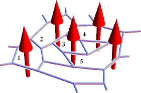
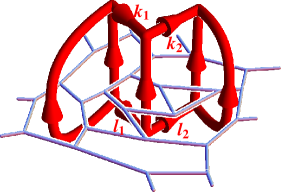
Figure 2: (color online) A flux-tube network represents quantum numbers of an elementary excitation with $N=5$ fluxons. The trivalent graph is the same as the one in Figure 1, and is assumed to be on a sphere.

The above numerical exact diagonalization shows that with the five occupied plaquettes fixed, there are more than one five-fluxon excitations. Therefore, the $n^{j}_{p}$’s are not enough to give the full set of quantum numbers for the degenerate five-fluxon states. Moreover, the numerical results also shows that the degeneracy does not depend the locations of the five occupied plaquettes. Thus the degeneracy is topological in nature, and this suggests that the quantum numbers, other than the $n^{j}_{p}$’s, that distinguish the degenerate five-fluxon states should be also topological in nature. Physically these extra quantum numbers, which we call as topological charges, describe relative degrees of freedom among the fluxons.

In Ref. Hu2, , we will show that the topological charges for five-fluxon states can be obtained by starting from the consideration of topological charges for a subsystem consisting of only two fluxons. It turns out that the topological charges of two fluxons can be classified by the quantum double charges of the Fibonacci data $\{j=0,j=1\}$. Following Ref. Wang ), we denote the string types $j=0$ and $j=1$ by $\mathbf{1}$ and $\tau$, respectively. Then the quantum double charges for a two-fluxon states are then denoted by $(\mathbf{1},\overline{\mathbf{1}})$, $(\tau,\overline{\mathbf{1}})$, $(\mathbf{1},\overline{\tau})$, and $(\tau,\overline{\tau})$.

The full set of quantum numbers for five-fluxon states in terms of quantum double charges can be represented by flux-tube networks as those shown in Fig. 2. In addition to $n^{\tau}_{p}=1$ for $p=1,2,\dots,5$, we have two more quantum numbers: the total topological charge $(k_{1}\overline{l_{1}})$ of the subsystem containing two fluxons at $p=1$ and $2$, and $(k_{2}\overline{l_{2}})$ of the subsystem containing three fluxons at $p=1,2$ and $3$. (These quantum numbers are defined in Hu2 , which we will not dwell on in this letter). Both of them take values in the quantum double charges, and can be thought as the flux connecting the $\tau$ flux through the five fixed plaquettes. In Fig. 2, we have five $\tau$ fluxes through the five fixed plaquettes, and the two $\tau$ fluxes through $p=1$ and $2$ couple to $k_{1}$ flux above the plane and to $l_{1}$ below the plane. The allowed values of $k_{1}$ and $l_{1}$ are constrained by the fusion rule $\delta_{\tau\tau k_{1}}=1$ and $\delta_{\tau\tau l_{1}}=1$, i.e., $k_{1},l_{1}=\mathbf{1},\tau$. The fluxes $k_{2}$ and $l_{2}$ result from coupling $k_{1}$ and $l_{1}$ to the $\tau$ flux through $p=3$.

This set of quantum numbers classify the degenerate five-fluxon states on a sphere, giving a basis

$$\left\{|{k_{1}\overline{l_{1}},k_{2}\overline{l_{2}}}\rangle\right\},\qquad\text{constrained by }\quad\delta_{\tau k_{1}k_{2}}=1,\delta_{\tau l_{1}l_{2}}=1.$$ (36)

$k_{1},k_{2}$ (or $l_{1},l_{2}$) take three possible values: $|{k_{1}=\mathbf{1},k_{2}=\tau}\rangle$, $|{k_{1}=\tau,k_{2}=\mathbf{1}}\rangle$, and $|{k_{1}=\tau,k_{2}=\tau}\rangle$. Therefore five-fluxon excitations (at five fixed plaquettes) have the degeneracy $(F_{5-1})^{2}=9$.

In general, $N$-fluxon excitations on a sphere have a basis labeled by $N-3$ quantum-double charges $|{k_{1}\overline{l_{1}},k_{2}\overline{l_{2}},\dots,k_{N-3}\overline{l_{N-3}}}\rangle$, constrained by $\delta_{\tau k_{n}k_{n+1}}=1$ and $\delta_{\tau l_{n}l_{n+1}}=1$. To view them clearly, we take the skeleton of the flux-tube network in Fig. 2 as the basis:

$$\begin{matrix}\lx@xy@svg{\hbox{\raise 0.0pt\hbox{\kern 0.0pt\hbox{\ignorespaces{}{\hbox{\kern 30.0pt\raise 24.0pt\hbox{\hbox{\kern 0.0pt\raise 0.0pt\hbox{\hbox{\lx@xy@point}}}}}}{}{\hbox{\kern 60.0pt\raise 24.0pt\hbox{\hbox{\kern 0.0pt\raise 0.0pt\hbox{\hbox{\lx@xy@point}}}}}}{}{}{}{\hbox{\kern 150.0pt\raise 24.0pt\hbox{\hbox{\kern 0.0pt\raise 0.0pt\hbox{\hbox{\lx@xy@point}}}}}}{}{}\ignorespaces\ignorespaces{\hbox{\lx@xy@droprule}}\ignorespaces{\hbox{\kern 15.0pt\raise 24.0pt\hbox{\hbox{\kern 0.0pt\raise 0.0pt\hbox{\lx@xy@tip{1}\lx@xy@tip{-1}}}}}}\ignorespaces{\hbox{\kern 13.46997pt\raise 30.0pt\hbox{\hbox{\kern 0.0pt\raise-1.50694pt\hbox{$\textstyle{\scriptstyle\tau}$}}}}}\ignorespaces\ignorespaces{\hbox{\lx@xy@droprule}}\ignorespaces{\hbox{\kern 30.0pt\raise 12.0pt\hbox{\hbox{\kern 0.0pt\raise 0.0pt\hbox{\lx@xy@tip{1}\lx@xy@tip{-1}}}}}}\ignorespaces{\hbox{\kern 34.46997pt\raise 6.0pt\hbox{\hbox{\kern 0.0pt\raise-1.50694pt\hbox{$\textstyle{\scriptstyle\tau}$}}}}}\ignorespaces\ignorespaces{\hbox{\lx@xy@droprule}}\ignorespaces{\hbox{\kern 60.0pt\raise 12.0pt\hbox{\hbox{\kern 0.0pt\raise 0.0pt\hbox{\lx@xy@tip{1}\lx@xy@tip{-1}}}}}}\ignorespaces{\hbox{\kern 64.46997pt\raise 6.0pt\hbox{\hbox{\kern 0.0pt\raise-1.50694pt\hbox{$\textstyle{\scriptstyle\tau}$}}}}}\ignorespaces\ignorespaces{\hbox{\lx@xy@droprule}}\ignorespaces{\hbox{\kern 150.0pt\raise 12.0pt\hbox{\hbox{\kern 0.0pt\raise 0.0pt\hbox{\lx@xy@tip{1}\lx@xy@tip{-1}}}}}}\ignorespaces{\hbox{\kern 154.46997pt\raise 6.0pt\hbox{\hbox{\kern 0.0pt\raise-1.50694pt\hbox{$\textstyle{\scriptstyle\tau}$}}}}}\ignorespaces\ignorespaces{\hbox{\lx@xy@droprule}}\ignorespaces{\hbox{\kern 165.0pt\raise 24.0pt\hbox{\hbox{\kern 0.0pt\raise 0.0pt\hbox{\lx@xy@tip{1}\lx@xy@tip{-1}}}}}}\ignorespaces{\hbox{\kern 163.46997pt\raise 30.0pt\hbox{\hbox{\kern 0.0pt\raise-1.50694pt\hbox{$\textstyle{\scriptstyle\tau}$}}}}}\ignorespaces\ignorespaces{\hbox{\lx@xy@droprule}}\ignorespaces{\hbox{\kern 45.0pt\raise 24.0pt\hbox{\hbox{\kern 0.0pt\raise 0.0pt\hbox{\lx@xy@tip{1}\lx@xy@tip{-1}}}}}}\ignorespaces{\hbox{\kern 42.06772pt\raise 30.0pt\hbox{\hbox{\kern 0.0pt\raise-1.78612pt\hbox{$\textstyle{\scriptstyle k_{1}}$}}}}}\ignorespaces\ignorespaces{\hbox{\lx@xy@droprule}}\ignorespaces{\hbox{\kern 75.0pt\raise 24.0pt\hbox{\hbox{\kern 0.0pt\raise 0.0pt\hbox{\lx@xy@tip{1}\lx@xy@tip{-1}}}}}}\ignorespaces{\hbox{\kern 72.06772pt\raise 30.0pt\hbox{\hbox{\kern 0.0pt\raise-1.78612pt\hbox{$\textstyle{\scriptstyle k_{2}}$}}}}}\ignorespaces\ignorespaces{\hbox{\lx@xy@droprule}}\ignorespaces{\hbox{\kern 135.0pt\raise 24.0pt\hbox{\hbox{\kern 0.0pt\raise 0.0pt\hbox{\lx@xy@tip{1}\lx@xy@tip{-1}}}}}}\ignorespaces{\hbox{\kern 129.57607pt\raise 30.0pt\hbox{\hbox{\kern 0.0pt\raise-1.74722pt\hbox{$\textstyle{\scriptstyle k_{N-3}}$}}}}}\ignorespaces{\hbox{\lx@xy@drawline@}}}}}}\end{matrix}\quad\otimes\quad\begin{matrix}\lx@xy@svg{\hbox{\raise 0.0pt\hbox{\kern 0.0pt\hbox{\ignorespaces{}{\hbox{\kern 30.0pt\raise 0.0pt\hbox{\hbox{\kern 0.0pt\raise 0.0pt\hbox{\hbox{\lx@xy@point}}}}}}{}{\hbox{\kern 60.0pt\raise 0.0pt\hbox{\hbox{\kern 0.0pt\raise 0.0pt\hbox{\hbox{\lx@xy@point}}}}}}{}{}{}{\hbox{\kern 150.0pt\raise 0.0pt\hbox{\hbox{\kern 0.0pt\raise 0.0pt\hbox{\hbox{\lx@xy@point}}}}}}{}{}\ignorespaces\ignorespaces{\hbox{\lx@xy@droprule}}\ignorespaces{\hbox{\kern 15.0pt\raise 0.0pt\hbox{\hbox{\kern 0.0pt\raise 0.0pt\hbox{\lx@xy@tip{1}\lx@xy@tip{-1}}}}}}\ignorespaces{\hbox{\kern 13.46997pt\raise 6.0pt\hbox{\hbox{\kern 0.0pt\raise-1.50694pt\hbox{$\textstyle{\scriptstyle\tau}$}}}}}\ignorespaces\ignorespaces{\hbox{\lx@xy@droprule}}\ignorespaces{\hbox{\kern 30.0pt\raise 12.0pt\hbox{\hbox{\kern 0.0pt\raise 0.0pt\hbox{\lx@xy@tip{1}\lx@xy@tip{-1}}}}}}\ignorespaces{\hbox{\kern 34.46997pt\raise 18.0pt\hbox{\hbox{\kern 0.0pt\raise-1.50694pt\hbox{$\textstyle{\scriptstyle\tau}$}}}}}\ignorespaces\ignorespaces{\hbox{\lx@xy@droprule}}\ignorespaces{\hbox{\kern 60.0pt\raise 12.0pt\hbox{\hbox{\kern 0.0pt\raise 0.0pt\hbox{\lx@xy@tip{1}\lx@xy@tip{-1}}}}}}\ignorespaces{\hbox{\kern 64.46997pt\raise 18.0pt\hbox{\hbox{\kern 0.0pt\raise-1.50694pt\hbox{$\textstyle{\scriptstyle\tau}$}}}}}\ignorespaces\ignorespaces{\hbox{\lx@xy@droprule}}\ignorespaces{\hbox{\kern 150.0pt\raise 12.0pt\hbox{\hbox{\kern 0.0pt\raise 0.0pt\hbox{\lx@xy@tip{1}\lx@xy@tip{-1}}}}}}\ignorespaces{\hbox{\kern 154.46997pt\raise 18.0pt\hbox{\hbox{\kern 0.0pt\raise-1.50694pt\hbox{$\textstyle{\scriptstyle\tau}$}}}}}\ignorespaces\ignorespaces{\hbox{\lx@xy@droprule}}\ignorespaces{\hbox{\kern 165.0pt\raise 0.0pt\hbox{\hbox{\kern 0.0pt\raise 0.0pt\hbox{\lx@xy@tip{1}\lx@xy@tip{-1}}}}}}\ignorespaces{\hbox{\kern 163.46997pt\raise 6.0pt\hbox{\hbox{\kern 0.0pt\raise-1.50694pt\hbox{$\textstyle{\scriptstyle\tau}$}}}}}\ignorespaces\ignorespaces{\hbox{\lx@xy@droprule}}\ignorespaces{\hbox{\kern 45.0pt\raise 0.0pt\hbox{\hbox{\kern 0.0pt\raise 0.0pt\hbox{\lx@xy@tip{1}\lx@xy@tip{-1}}}}}}\ignorespaces{\hbox{\kern 42.88681pt\raise 6.0pt\hbox{\hbox{\kern 0.0pt\raise-1.78612pt\hbox{$\textstyle{\scriptstyle l_{1}}$}}}}}\ignorespaces\ignorespaces{\hbox{\lx@xy@droprule}}\ignorespaces{\hbox{\kern 75.0pt\raise 0.0pt\hbox{\hbox{\kern 0.0pt\raise 0.0pt\hbox{\lx@xy@tip{1}\lx@xy@tip{-1}}}}}}\ignorespaces{\hbox{\kern 72.88681pt\raise 6.0pt\hbox{\hbox{\kern 0.0pt\raise-1.78612pt\hbox{$\textstyle{\scriptstyle l_{2}}$}}}}}\ignorespaces\ignorespaces{\hbox{\lx@xy@droprule}}\ignorespaces{\hbox{\kern 135.0pt\raise 0.0pt\hbox{\hbox{\kern 0.0pt\raise 0.0pt\hbox{\lx@xy@tip{1}\lx@xy@tip{-1}}}}}}\ignorespaces{\hbox{\kern 130.39516pt\raise 6.0pt\hbox{\hbox{\kern 0.0pt\raise-1.74722pt\hbox{$\textstyle{\scriptstyle l_{N-3}}$}}}}}\ignorespaces{\hbox{\lx@xy@drawline@}}}}}}\end{matrix}, \textstyle{\scriptstyle\tau} \textstyle{\scriptstyle\tau} \textstyle{\scriptstyle\tau} \textstyle{\scriptstyle\tau} \textstyle{\scriptstyle\tau} \textstyle{\scriptstyle k_{1}} \textstyle{\scriptstyle k_{2}} \textstyle{\scriptstyle k_{N-3}} \textstyle{\scriptstyle\tau} \textstyle{\scriptstyle\tau} \textstyle{\scriptstyle\tau} \textstyle{\scriptstyle\tau} \textstyle{\scriptstyle\tau} \textstyle{\scriptstyle l_{1}} \textstyle{\scriptstyle l_{2}} \textstyle{\scriptstyle l_{N-3}} \textstyle{\scriptstyle\tau} \textstyle{\scriptstyle\tau} \textstyle{\scriptstyle\tau} \textstyle{\scriptstyle\tau} \textstyle{\scriptstyle\tau} \textstyle{\scriptstyle k_{1}} \textstyle{\scriptstyle k_{2}} \textstyle{\scriptstyle k_{N-3}} \textstyle{\scriptstyle\tau} \textstyle{\scriptstyle\tau} \textstyle{\scriptstyle\tau} \textstyle{\scriptstyle\tau} \textstyle{\scriptstyle\tau} \textstyle{\scriptstyle l_{1}} \textstyle{\scriptstyle l_{2}} \textstyle{\scriptstyle l_{N-3}}$$ (37)

where the left part corresponds to the flux-tube network above the plane, and the right part to the one below the plane. The external links correspond to the flux tubes through the plaquettes. The basis depends on the ordering of the $N$ fluxons. In Fig. 2, if we choose different ordering of fluxons at the five plaquettes, the basis (37) will give a flux-tube network different from the one in Fig. 2(b). However, this ordering of the fluxons can be fixed once for all. All different choices of basis are equivalent up to a unitary basis transformation, due to the topology symmetry of the states. (See the mutation symmetry in Ref. GSD, ). The exclusion statistics can be conveniently analyzed in the above basis. (The details are left to the forthcoming paper Hu2, .)

The above analysis can be generalized to the case on a torus. The nontrivial topology introduce two loops in the basis. The $N$-fluxon basis is expressed by

$$\lx@xy@svg{\hbox{\raise 0.0pt\hbox{\kern 0.0pt\hbox{\ignorespaces{\hbox{\kern 30.0pt\raise 0.0pt\hbox{\hbox{\kern 0.0pt\raise 0.0pt\hbox{\hbox{\lx@xy@point}}}}}}{}{\hbox{\kern 60.0pt\raise 0.0pt\hbox{\hbox{\kern 0.0pt\raise 0.0pt\hbox{\hbox{\lx@xy@point}}}}}}{}{}{}{\hbox{\kern 150.0pt\raise 0.0pt\hbox{\hbox{\kern 0.0pt\raise 0.0pt\hbox{\hbox{\lx@xy@point}}}}}}{}\ignorespaces\ignorespaces{\hbox{\lx@xy@droprule}}\ignorespaces{\hbox{\kern 30.0pt\raise-12.0pt\hbox{\hbox{\kern 0.0pt\raise 0.0pt\hbox{\lx@xy@tip{1}\lx@xy@tip{-1}}}}}}\ignorespaces{\hbox{\kern 34.46997pt\raise-6.0pt\hbox{\hbox{\kern 0.0pt\raise-1.50694pt\hbox{$\textstyle{\scriptstyle\tau}$}}}}}\ignorespaces\ignorespaces{\hbox{\lx@xy@droprule}}\ignorespaces{\hbox{\kern 60.0pt\raise-12.0pt\hbox{\hbox{\kern 0.0pt\raise 0.0pt\hbox{\lx@xy@tip{1}\lx@xy@tip{-1}}}}}}\ignorespaces{\hbox{\kern 64.46997pt\raise-6.0pt\hbox{\hbox{\kern 0.0pt\raise-1.50694pt\hbox{$\textstyle{\scriptstyle\tau}$}}}}}\ignorespaces\ignorespaces{\hbox{\lx@xy@droprule}}\ignorespaces{\hbox{\kern 150.0pt\raise-12.0pt\hbox{\hbox{\kern 0.0pt\raise 0.0pt\hbox{\lx@xy@tip{1}\lx@xy@tip{-1}}}}}}\ignorespaces{\hbox{\kern 154.46997pt\raise-6.0pt\hbox{\hbox{\kern 0.0pt\raise-1.50694pt\hbox{$\textstyle{\scriptstyle\tau}$}}}}}\ignorespaces\ignorespaces{\hbox{\lx@xy@droprule}}\ignorespaces{\hbox{\kern 45.0pt\raise 0.0pt\hbox{\hbox{\kern 0.0pt\raise 0.0pt\hbox{\lx@xy@tip{1}\lx@xy@tip{-1}}}}}}\ignorespaces{\hbox{\kern 42.06772pt\raise 6.0pt\hbox{\hbox{\kern 0.0pt\raise-1.78612pt\hbox{$\textstyle{\scriptstyle k_{1}}$}}}}}\ignorespaces\ignorespaces{\hbox{\lx@xy@droprule}}\ignorespaces{\hbox{\kern 75.0pt\raise 0.0pt\hbox{\hbox{\kern 0.0pt\raise 0.0pt\hbox{\lx@xy@tip{1}\lx@xy@tip{-1}}}}}}\ignorespaces{\hbox{\kern 72.06772pt\raise 6.0pt\hbox{\hbox{\kern 0.0pt\raise-1.78612pt\hbox{$\textstyle{\scriptstyle k_{2}}$}}}}}\ignorespaces\ignorespaces{\hbox{\lx@xy@droprule}}\ignorespaces{\hbox{\kern 135.0pt\raise 0.0pt\hbox{\hbox{\kern 0.0pt\raise 0.0pt\hbox{\lx@xy@tip{1}\lx@xy@tip{-1}}}}}}\ignorespaces{\hbox{\kern 129.57607pt\raise 6.0pt\hbox{\hbox{\kern 0.0pt\raise-1.74722pt\hbox{$\textstyle{\scriptstyle k_{N-1}}$}}}}}\ignorespaces{\hbox{\lx@xy@drawline@}}\ignorespaces\hbox{\hbox{\kern 0.0pt\raise 0.0pt\hbox{{}{}{}{{}{}}\ignorespaces\ignorespaces{{}{}{}{}\ignorespaces{}\lx@xy@spline@}{{}{}{}\lx@xy@spline@}{}}}}\ignorespaces{}{}{}{}{}{{}}{\hbox{\kern 90.0pt\raise 27.0pt\hbox{\hbox{\kern 0.0pt\raise 0.0pt\hbox{\lx@xy@tip{1}\lx@xy@tip{-1}}}}}}\ignorespaces{\hbox{\kern 88.23906pt\raise 33.0pt\hbox{\hbox{\kern 0.0pt\raise-0.8264pt\hbox{$\textstyle{\scriptstyle p}$}}}}}}}}}\quad\otimes\quad\lx@xy@svg{\hbox{\raise 0.0pt\hbox{\kern 0.0pt\hbox{\ignorespaces{\hbox{\kern 30.0pt\raise 0.0pt\hbox{\hbox{\kern 0.0pt\raise 0.0pt\hbox{\hbox{\lx@xy@point}}}}}}{}{\hbox{\kern 60.0pt\raise 0.0pt\hbox{\hbox{\kern 0.0pt\raise 0.0pt\hbox{\hbox{\lx@xy@point}}}}}}{}{}{}{\hbox{\kern 150.0pt\raise 0.0pt\hbox{\hbox{\kern 0.0pt\raise 0.0pt\hbox{\hbox{\lx@xy@point}}}}}}{}\ignorespaces\ignorespaces{\hbox{\lx@xy@droprule}}\ignorespaces{\hbox{\kern 30.0pt\raise 12.0pt\hbox{\hbox{\kern 0.0pt\raise 0.0pt\hbox{\lx@xy@tip{1}\lx@xy@tip{-1}}}}}}\ignorespaces{\hbox{\kern 34.46997pt\raise 18.0pt\hbox{\hbox{\kern 0.0pt\raise-1.50694pt\hbox{$\textstyle{\scriptstyle\tau}$}}}}}\ignorespaces\ignorespaces{\hbox{\lx@xy@droprule}}\ignorespaces{\hbox{\kern 60.0pt\raise 12.0pt\hbox{\hbox{\kern 0.0pt\raise 0.0pt\hbox{\lx@xy@tip{1}\lx@xy@tip{-1}}}}}}\ignorespaces{\hbox{\kern 64.46997pt\raise 18.0pt\hbox{\hbox{\kern 0.0pt\raise-1.50694pt\hbox{$\textstyle{\scriptstyle\tau}$}}}}}\ignorespaces\ignorespaces{\hbox{\lx@xy@droprule}}\ignorespaces{\hbox{\kern 150.0pt\raise 12.0pt\hbox{\hbox{\kern 0.0pt\raise 0.0pt\hbox{\lx@xy@tip{1}\lx@xy@tip{-1}}}}}}\ignorespaces{\hbox{\kern 154.46997pt\raise 18.0pt\hbox{\hbox{\kern 0.0pt\raise-1.50694pt\hbox{$\textstyle{\scriptstyle\tau}$}}}}}\ignorespaces\ignorespaces{\hbox{\lx@xy@droprule}}\ignorespaces{\hbox{\kern 45.0pt\raise 0.0pt\hbox{\hbox{\kern 0.0pt\raise 0.0pt\hbox{\lx@xy@tip{1}\lx@xy@tip{-1}}}}}}\ignorespaces{\hbox{\kern 42.88681pt\raise 6.0pt\hbox{\hbox{\kern 0.0pt\raise-1.78612pt\hbox{$\textstyle{\scriptstyle l_{1}}$}}}}}\ignorespaces\ignorespaces{\hbox{\lx@xy@droprule}}\ignorespaces{\hbox{\kern 75.0pt\raise 0.0pt\hbox{\hbox{\kern 0.0pt\raise 0.0pt\hbox{\lx@xy@tip{1}\lx@xy@tip{-1}}}}}}\ignorespaces{\hbox{\kern 72.88681pt\raise 6.0pt\hbox{\hbox{\kern 0.0pt\raise-1.78612pt\hbox{$\textstyle{\scriptstyle l_{2}}$}}}}}\ignorespaces\ignorespaces{\hbox{\lx@xy@droprule}}\ignorespaces{\hbox{\kern 135.0pt\raise 0.0pt\hbox{\hbox{\kern 0.0pt\raise 0.0pt\hbox{\lx@xy@tip{1}\lx@xy@tip{-1}}}}}}\ignorespaces{\hbox{\kern 130.39516pt\raise 6.0pt\hbox{\hbox{\kern 0.0pt\raise-1.74722pt\hbox{$\textstyle{\scriptstyle l_{N-1}}$}}}}}\ignorespaces{\hbox{\lx@xy@drawline@}}\ignorespaces\hbox{\hbox{\kern 0.0pt\raise 0.0pt\hbox{{}{}{}{{}{}}\ignorespaces\ignorespaces{{}{}{}{}\ignorespaces{}\lx@xy@spline@}{{}{}{}\lx@xy@spline@}{}}}}\ignorespaces{}{}{}{}{}{{}}{\hbox{\kern 90.0pt\raise-27.0pt\hbox{\hbox{\kern 0.0pt\raise 0.0pt\hbox{\lx@xy@tip{1}\lx@xy@tip{-1}}}}}}\ignorespaces{\hbox{\kern 88.31198pt\raise-21.0pt\hbox{\hbox{\kern 0.0pt\raise-0.8264pt\hbox{$\textstyle{\scriptstyle q}$}}}}}}}}}. \textstyle{\scriptstyle\tau} \textstyle{\scriptstyle\tau} \textstyle{\scriptstyle\tau} \textstyle{\scriptstyle k_{1}} \textstyle{\scriptstyle k_{2}} \textstyle{\scriptstyle k_{N-1}} \textstyle{\scriptstyle p} \textstyle{\scriptstyle\tau} \textstyle{\scriptstyle\tau} \textstyle{\scriptstyle\tau} \textstyle{\scriptstyle l_{1}} \textstyle{\scriptstyle l_{2}} \textstyle{\scriptstyle l_{N-1}} \textstyle{\scriptstyle q} \textstyle{\scriptstyle\tau} \textstyle{\scriptstyle\tau} \textstyle{\scriptstyle\tau} \textstyle{\scriptstyle k_{1}} \textstyle{\scriptstyle k_{2}} \textstyle{\scriptstyle k_{N-1}} \textstyle{\scriptstyle p} \textstyle{\scriptstyle\tau} \textstyle{\scriptstyle\tau} \textstyle{\scriptstyle\tau} \textstyle{\scriptstyle l_{1}} \textstyle{\scriptstyle l_{2}} \textstyle{\scriptstyle l_{N-1}} \textstyle{\scriptstyle q}$$ (38)

Again, this can be viewed as the skeleton of the flux-tube network through plaquettes of a torus graph, with left part corresponding to the layer outside the torus surface while the right one inside the torus surface. If we imagine the embedding of the torus surface into the $S^{3}$ manifold, we see that $S^{3}$ is cut along the surface into two solid torus, giving rise to the two non-contractible loops in the above basis. We can apply similar analysis as in the sphere case: now in formula (Emergent Exclusion Statistics of Fibonacci Anyons in 2D Topological Phases), $N_{1}=0,1$ stands for the number of $p=\mathbf{1}$ (and $N_{2}$ for the number of $q=\mathbf{1}$). The mutual exclusion $\alpha_{31}=2=\alpha_{42}$ survives because of the exclusion between $p=0$ and $k_{1}=0$ (or $k_{N-1}$=0).

In particular, the ground states have four-fold degeneracy, with the basis $|{p,q}\rangle$ as special example of the formula (38).

References

(1) “Fractional Statistics and Anyon Superconductivity”, ed. F.
Wilczek, (World Scientific, 1990).
(2) Y.S. Wu, Phys. Rev. Lett. 73, 922 (1994).
(3) F.D.M. Haldane, Phys. Rev. Lett. 67, 937 (1991).
(4) For thermodynamics of a single species of abelian anyons (with no mutual
statistics), see S. B. Isakov, Int. J. Mod. Phys. A9, 2563 (1994); A. Dasnieres de
Veigy et al, Phys. Rev. Lett. 72, 600 (1994).
(5) Y.S. Wu, “Fractional Statistics and Strongly
Correlated Systems”, in “Topics in Theoretical Physics”, ed.
Y.M. Cho, (World Scientific, 1996); pp. 27-59.
(6) D. Bernard, Y.S. Wu, in “New Developments of
Integrable Systems and Long-Range Interaction Models”, ed. M.L Ge
and Y.S. Wu, (World Scientific, 1995); pp. 10-21.
(18) N. Read, E. Rezayi, Phys. Rev. B 59, 8084 (1999).
(19) I. Lesanovsky, H. Katsura, Phys. Rev. A 86, 041601(R)
(2012).
(20) S. Guruswamy, K. Schoutens, Nucl. Phys. B 556, 530
(1999).
(21) M. Freedman, C. Nayak, K. Shtengel, K. Walker, Z. Wang, Ann. Phys. 310, 428 (2004).
(22) See the suppelementary material.
(23) M. D. Schulz, S. Dusuel, K. P. Schmidt, J. Vidal, Phys. Rev. Lett. 110,
147203 (2013).
(24) A different state-counting formula appeared in ref. Vidal, for the particular case with Fibonacci data, but no connection to exclusion statistics was made.
(25) Y. Hu, S. Stirling, Y.S. Wu, Phys. Rev. B 85, 075107
(2012).