Numerical simulation of ejected molten metal-nanoparticles liquefied by laser irradiation: Interplay of geometry and dewetting

Abstract

Metallic nanoparticles, liquefied by fast laser irradiation, go through a rapid change of shape attempting to minimize their surface energy. The resulting nanodrops may be ejected from the substrate when the mechanisms leading to dewetting are sufficiently strong, as in the experiments involving gold nanoparticles [Habenicht et al., Science 309, 2043 (2005)]. We use a direct continuum-level approach to accurately model the process of liquid nanodrop formation and the subsequent ejection from the substrate. Our computations show a significant role of inertial effects and an elaborate interplay of initial geometry and wetting properties: e.g., we can control the direction of ejection by prescribing appropriate initial shape and/or wetting properties. The basic insight regarding ejection itself can be reached by considering a simple effective model based on an energy balance. We validate our computations by comparing directly with the experiments specified above involving the length scales measured in hundreds of nanometers, and with molecular dynamics simulations on much shorter scales measured in tens of atomic diameters, as in M. Fuentes-Cabrera et al., Phys. Rev. E 83, 041603 (2011). The quantitative agreement, in addition to illustrating how to controlling particle ejection, shows utility of continuum-based simulation in describing dynamics on nanoscale quantitatively, even in a complex setting as considered here.

Evolution of fluid drops deposited on solid substrates has been a focus of large research effort for decades. More recently, this effort has been particularly extensive on the nanoscale, due to relevance of nanostructures in a variety of fields, ranging from DNA sequencing to plasmonics Maier (2007); Atwater and Polman (2010), nanogmagnetism Baderi (2006), and liquid crystal displays and solar panel designs Maier et al. (2003). For example, the size and distribution of metallic particles strongly affects the coupling of surface plasmons to incident energy Maier (2007). Controlling this coupling has the potential for large increases in the yield of solar cell devices.

In addition to physical experiments, modeling and simulations provide a significant insight into the effects governing the evolution of drops and other liquid structures. Numerical simulation has an advantage of allowing to switch off some of the involved physical phenomena and therefore isolate the dominant ones. On nanoscale, however, it is not trivial to decide on appropriate simulation technique. Molecular dynamics (MD) simulations, while very powerful and presumably as close to real physical picture as it is our knowledge of underlying interaction laws, are still extremely computationally demanding. Therefore, one would like to resort to the continuum-based simulation. However, it is not immediately clear that this approach is appropriate on the nanoscale where the basic assumptions of continuum fluid mechanics are pushed to their limits. In addition, the continuum simulation of free surface time-dependent problems based on full three-dimensional Navier-Stokes (N-S) formulation is still computationally demanding. For this reason, this type of simulation is rarely attempted in practice and instead the researchers resort to asymptotic (long-wave) methods. Such an approach has been applied with success to problems involving wetting and dewetting of drops and films; see Oron et al. (1997) for reviews. This direction is, however, questionable due to the inherent assumptions, in particular when contact angles are large and inertial effects are significant. One such class of problems involves liquid metals. These configurations may even lead to topological changes under liquefaction with metal particles detaching from the substrate Habenicht et al. (2005). In such cases, long-wave theory clearly cannot be applied.

In this work, we show that direct numerical solutions of N-S equations lead to the results which are in quantitative agreement with (i) MD simulations of dewetting of $1$-$1.5$ nm thick, liquid copper (Cu) disks of radius of $10$-$15$ nm, and (ii) physical experiments involving ‘jumping’ gold (Au) nanoparticles of typical in-plane length scale in the range of $100$ nanometers. While utility of continuum mechanics on nanoscale problems involving liquid metals was discussed previously (see, e.g., Burton et al. (2004)), as far as the authors are aware, this is the first attempt to compare explicitly continuum N-S simulations both to MD and to physical experiments in a dynamic setting. Furthermore, we utilize the simulations to illustrate the dominant effects and discuss in particular the conditions leading to ejection of fluid material from the substrate. We also present an effective model based on an energy balance to provide a basic insight into the ejection mechanism. We first consider dewetting of liquid Cu disks recently simulated by MD Fuentes-Cabrera et al. (2011) and then shift focus to Au particles considered experimentally Habenicht et al. (2005).

Methods. The simulations are based on the Volume of Fluid (VoF) approach, which, when coupled to a flow solver, is also used to compute quantities related to surface tension that enter the flow calculation. Until recently, the VoF method was not deemed appropriate for the study of phenomena in which surface tension is the driving force. Recent improvements to calculating curvature and applying the surface tension force appear to resolve this issue Sussman (2003). Within this approach, one solves the three-dimensional N-S equations that govern the motion of the fluid both inside of the liquid domain, and in the surrounding gas phase. For Cu disk structures, a free-slip boundary condition is specified at the substrate; this choice is motivated by the MD simulations Fuentes-Cabrera et al. (2011). This assumption is also consistent with the fact that the length scale associated with slip is nanometric for most systems Bonn et al. (2009). When considering Au structures, the Navier slip Haley and Miksis (1991) with slip length of $3$ nm is imposed; this particular value is obtained by direct comparison with the experiments Habenicht et al. (2005) and is further discussed in Supplementary Materials sup . Such a value is also consistent with the MD simulations Qian et al. (2004), indicating slip lengths of a few nanometers for mesoscopic systems. The physical problem considered is the one of a Newtonian, isothermal, incompressible fluid and therefore in the present work we do not consider the effects related to phase change and/or thermal variation of material properties occurring in experiments Habenicht et al. (2005). Simulations are carried out on an adaptive mesh Popinet (2003), and numerical convergence has been verified by considering simulations with different grid resolutions Afkhami et al. (2009). See sup for more details.

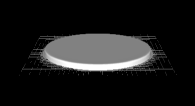
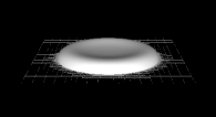
0 ps	20 ps
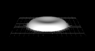
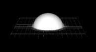
30 ps	200 ps
	(a)

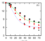
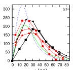
Figure 1: (Color online) Evolution of a Cu disk ($h_{0}=15$ Å, $R_{0}=150$ Å, $\theta_{0}=90^{\circ}$); (a) Snapshots for $\theta_{\text{eq}}=80{{}^{\circ}}$; (b) $R(t)$ and (c) $\dot{R}(t)$ for ($\blacksquare$) $\theta_{\text{eq}}=80{{}^{\circ}}$ and ($\blacktriangle$) $\theta_{\text{eq}}=115{{}^{\circ}}$. MD simulations for ($\bullet$) LJ-a, $\theta_{\text{eq}}=116{{}^{\circ}}$, and ($\blacklozenge$) LJ-b, $\theta_{\text{eq}}=75.6{{}^{\circ}}$, with $h_{0}=10$ Å and ($\blacktriangle$) LJ-b with $h_{0}=15$ Å Fuentes-Cabrera et al. (2011). Predictions of the model, Eq. (1), for $\theta_{\text{eq}}=80^{\circ}$ (solid green line) and $115^{\circ}$ (dashed blue line). $Oh\approx 0.35$.

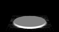
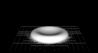
0 ps	20 ps
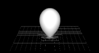
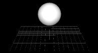
100 ps	190 ps
	(a)

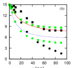
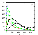
Figure 2: (Color online) Evolution of a disk ($h_{0}=15$ Å, $R_{0}=150$ Å, $\theta_{0}=90^{\circ}$); (a) for $\theta_{\text{eq}}=140{{}^{\circ}}$, the disk detaches at around $100$ ps (see also the animation in sup ); (b) $R(t)$ and (c) $\dot{R}(t)$ for $\theta_{\text{eq}}=80{{}^{\circ}}$ ($\blacksquare$)/($\blacksquare$) and $140{{}^{\circ}}$ ($\bullet$)/($\bullet$) when $Oh\approx 0.35$ (black) and $Oh\approx 1.1$ (green). Predictions of the model, Eq. (1), for $\theta_{\text{eq}}=80^{\circ}$ (solid red line) and $\theta_{\text{eq}}=140^{\circ}$ (dashed blue line) when $Oh\approx 1.1$.

Results. Figure 1(a) shows the evolution of a Cu disk of initial height $h_{0}=15$ Å and radius $R_{0}=150$ Å with an initial contact angle $\theta_{0}=90^{\circ}$, when the equilibrium contact angle $\theta_{\text{eq}}=80^{\circ}$, that dewetts and collapses into a spherical cap. Figure 1(b) and (c) show the front position, $R(t)$, and velocity, $\dot{R}(t)$, respectively. We also show the results of the MD simulations obtained by employing two different Lennard-Jones (LJ) potentials, LJ-a and LJ-b, that differ by the depth of potential well Fuentes-Cabrera et al. (2011). These results show that our numerical results and the MD simulations yield fully consistent retraction time scales. We also see that $\theta_{\text{eq}}$ influences the initial rapid retraction, with larger $\theta_{\text{eq}}$ leading to faster dynamics for early times.

A different type of evolution occurs if $\theta_{\text{eq}}$ is further increased. To illustrate this, Fig. 2(a) shows snapshots of the profiles for $h_{0}=15$ Å, $R_{0}=150$ Å, $\theta_{0}=90^{\circ}$, and $\theta_{\text{eq}}=140^{\circ}$. For this $\theta_{\text{eq}}$, the contraction is so fast that the nanodrop jumps off the surface, following elongation in the $y$ direction (normal to the substrate). Similar behavior is observed for any $\theta_{\text{eq}}\gtrsim 130^{\circ}$, again in quantitative agreement with the MD simulations Fuentes-Cabrera et al. (2011).

To gain additional insight regarding the effects that drive contraction, and possibly ejection of the fluid, we have carried out additional set of simulations with modified inertial effects. This was implemented by varying incompressible fluid density, but more generally the dynamics can be characterized by Ohnesorge number, $Oh=\eta/\sqrt{\rho\sigma R_{0}}$, which is related to the Reynolds number defined based on a characteristic capillary velocity, $\sigma/\eta$, as $Re=Oh^{-2}$. For liquid Cu results in Fig. 1, $Oh\approx 0.35$, suggesting that inertial effects are important; the same conclusion can be reached by considering an intrinsic length scale, $\ell_{v}=\eta^{2}/(\rho\sigma)$, above which inertial effects become significant; for liquid Cu, $\ell_{v}\approx 1.78$ nm, therefore smaller than typical length scales considered here. As an example, Fig. 2(b) and (c) show $R(t)$ and $\dot{R}(t)$ for $Oh\approx 0.35$ and $Oh\approx 1.1$. Reduced inertial effects eliminate the most noticeable feature of the dewetting: nanodroplets do not detach from the surface for the same $\theta_{\text{eq}}$. Additional simulations have shown that even for $\theta_{\text{eq}}=150^{\circ}$ there is no detachment for $Oh\approx 1.1$.

A basic understanding of the effects that drive the fluid evolution can be reached by a relatively simple effective model based on the balance of relevant energies. In this model, the evolution of the nanodisk obeys the energy balance equation

$$\frac{\partial}{\partial t}\left[E_{k}+E_{s}\right]+D=0~{},$$ (1)

where $E_{k}$, $E_{s}$ are the kinetic and surface energy, respectively, and $D$ is the rate of energy loss due to viscous dissipation, neglecting the gravitational energy. In this model, we describe the nanodisk dynamics by a fluid cylinder evolving on a solid substrate; a similar model has been considered for a drop impact problem Kim and Chun (2001). Here, $E_{k}={\rho\int_{\Omega}|\vec{V}|^{2}d\,\Omega/2}$ where the integration is over the fluid cylinder, and $\vec{V}=\vec{V}(\vec{x},t)$ is the axially symmetric fluid velocity. Using Young’s law Young (1805), $E_{s}=\sigma\left[\pi R(t)^{2}(1-\cos\theta_{\text{eq}})+2\pi R(t)h(t)\right]$, where $R(t)$ is the wetted radius and $h(t)$ is the cylinder height. The viscous dissipation energy $D=\int_{\Omega}(\tilde{\tau}:\nabla\vec{V})d\,\Omega$, where $\tilde{\tau}$ is the shear stress tensor. Using axisymmetric stagnation point flow and the conservation of mass, Eq. (1) reduces to a nonlinear second-order variable-coefficient ordinary differential equation given in sup . This equation is then solved numerically, and the results are shown together with the computational results in Figs. 1 and 2 (plane lines). We find very reasonable degree of agreement, suggesting that this simple model captures well the main mechanisms driving fluid contraction.

Figure 3 shows additional comparison between the numerical simulation and the effective model. In Fig. 3(a), we observe that both the simulations and the model, Eq. (1), predict approximately linear dependence of the ejection velocity on $\cos\theta_{\text{eq}}$. We expect that the discrepancy between the two is maily due to the deficiency of the model for large $\theta_{\text{eq}}$ sup . Figure 3(b) show a phase diagram in $(Oh,~{}\theta_{\text{eq}})$ parameter space illustrating the criteria for ejection resulting from the model, together with the results of the numerical simulation, concentrating here on small values of $Oh$. Although the model underpredicts $\theta_{\text{eq}}$ required for ejection, we note a consistent trend of the results. Note that for large $Oh\approx 1.1$ considered previously, both the model and the simulation are in non-detaching regime. Further investigation of the results of the model suggests that the ejection velocity increases approximately linearly as $Oh$ decreases when $\theta_{\text{eq}}$ is fixed (see sup for more details).

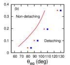
Figure 3: (Color online) (a) The effect of $\theta_{\text{eq}}$ on the ejection velocity, $V_{d}$, for a Cu nanodisk ($h_{0}=15$ Å, $R_{0}=150$ Å) predicted by the model based on Eq. (1) ($\blacktriangle$), see also Eq. (13) in sup , and simulations ($\blacksquare$). (b) Phase diagram showing the influence of $Oh$ and $\theta_{\text{eq}}$ on the ejection. The solid line is based on the model, Eq. (1), see also Eq. (13) in sup , and the symbols mark the result of the numerical simulation showing detaching ($\blacksquare$) and non-detaching ($\blacktriangle$) nanodrops. A linear fit to the solid line yields a slope of $0.0075$.

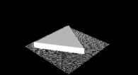
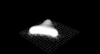
$0$ ns	$1.5$ ns
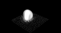
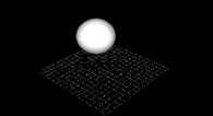
$4$ ns	$10$ ns

Figure 4: Evolution of a Au equilateral triangle ($a=405$ nm, $h_{0}=47$ nm, $\theta_{0}=90^{\circ}$, and $\theta_{\text{eq}}=140^{\circ}$). The structure collapses into a droplet and detaches at $t\approx 7$ ns (see also the animation in sup ).

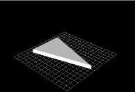
0 ns	0.6 ns
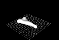
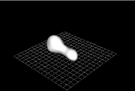
0.9 ns	2 ns
5 ns	7.4 ns

Figure 5: Evolution of a Au isosceles triangle for $h_{0}=24$ nm, $\theta_{0}=90^{\circ}$, long sides $a=438$ nm and short side $b=247$ nm; $\theta_{\text{eq}}=140^{\circ}$. The triangle collapses into a droplet and detaches from the substrate at around 5 ns (see also the animation in sup ).

Next we consider the configuration representative of physical experiments where Au triangular structures were liquefied and let to evolve on SiO₂ substrate Habenicht et al. (2005). Figure 4 shows the snapshots of initially equilateral triangle ($\theta_{0}=90^{\circ}$). The dewetting process first starts at the vertices, where the curvature is high. Due to high surface tension and large $\theta_{\text{eq}}$, the fluid starts to accumulate there. The humps at the vertices then coalesce into a droplet. Owing to a low viscosity of liquid gold, inertial effects dominate over viscous dissipation (here $Oh\approx 0.047$ sup ), giving rise to an upward movement that leads to droplet detaching from the surface with a velocity of $\approx 24$ m s^-1. This process is consistent with the dewetting induced ejection mechanism outlined in Habenicht et al. (2005). We note the consistency of the time scales found by the simulations and the experiments in Habenicht et al. (2005), where an ejection time scale of the order of $10$ ns was observed. In addition to comparing favorably with experiments, the simulations allow for an additional insight since it is possible to explore very fast time scales, and also easily vary the parameters, such as $\theta_{\text{eq}}$ and the initial shape, and ask what is their influence on the outcome.

Figure 6: $x$-$y$ cross sections of Au isosceles triangles for $h_{0}=24$ nm and $\theta_{0}=90^{\circ}$; (a-b) $a=438$ nm and $b=247$ nm for (a) $\theta_{\text{eq}}=130^{\circ}$, (b) $140^{\circ}$, showing the increase of ejection angle, $\alpha$, as $\theta_{\text{eq}}$ is increased (note that in (a), $\alpha=0$); (c-d) $\theta_{\text{eq}}=145^{\circ}$, and (c) $a=362$ nm, $b=185$ nm, (d) $a=475$ nm, $b=308$ nm; $t=0,~{}0.6,~{}1.2,~{}3,~{}4.4,~{}11,~{}19,~{}35$ ns. (e-f) Ejection angle $\alpha$ versus the $\theta_{eq}$ (e), when $a/b\approx 1.77$, and the initial geometrical ratio $a/b$ (f), when $\theta_{\text{eq}}=145^{\circ}$.

To illustrate the influence of geometry, we consider isosceles triangles. Figure 5 shows a perhaps unexpected result, that despite the fact that the vertex at the smallest angle collapses the fastest due to a higher curvature, the vertices at the larger angles arrive sooner to the center (future work should analyze how general this result is). This mismatch excites oscillations of the droplet translating into a tumbling movement after the ejection.

Next, we ask whether the ejection angle, $\alpha$, is always $\pi/2$. We find that $\alpha$ can be influenced for asymmetric collapse, and present two means for controlling it by modifying: (i) $\theta_{\text{eq}}$ and (ii) the initial geometry. Figure 6(a-b) shows that increasing $\theta_{\text{eq}}$ alters the no-ejection ($\alpha=0$) to a directional ejection ($0\leq\alpha\leq{\pi/2}$). A qualitative understanding can be reached by recalling that $\alpha\neq{\pi/2}$ is due to the lack of synhronicity of the collapse. A larger $\theta_{\text{eq}}$ results in higher surface energy, speeding up the fluid at the vertices. Therefore for larger $\theta_{\text{eq}}$, collapse is more synchronous and $\alpha$ is closer to $\pi/2$. For smaller $\theta_{\text{eq}}$, $\alpha$ may vanish (see Figure 6(a)), i.e. ejection does not happen, while an equilateral triangle with the same $\theta_{\text{eq}}$ does eject, illustrating the effect of asymmetry. We next consider the aspect ratio of the lengths, ($a,b$), of triangle sides, and find that the larger $a/b$ ratios lead to increased asymmetry of the collapse and smaller $\alpha$, as shown in Fig. 6(c-d).

Figures 6(e) and (f) show $\alpha$ versus $\theta_{\text{eq}}$ for fixed $a/b$, and versus $a/b$ for fixed $\theta_{\text{eq}}$, respectively. In Fig. 6(e) we see that the ejection angle increases monotonically with an increase of $\theta_{\text{eq}}$ with no ejection for $\theta_{\text{eq}}\lesssim 135^{\circ}$. Figure 6(f) shows that $\alpha$ decreases with increased asymmetry and that for the considered $\theta_{\text{eq}}$, the ejection does not occur, i.e. $\alpha=0$, when $a/b\gtrsim 2.4$. Very large ratios lead to a different type of dynamics: Rayleigh-Plateau type of breakup, see Kondic et al. (2009) for discussion in the context of liquid metals. More elaborate analysis of the influence of geometry and wetting properties is needed to fully understand the dynamics - we leave this for future work.

Conclusions. In this work, we have demonstrated that continuum simulations provide a good qualitative agreement with both MD simulations on the length scales in the range of $1$-$10$ nm, and with the physical experiments with in-plane length scales measured in the range of $100$ nanometers. We expect that this finding will further motivate modeling and computational work on these scales, since it is suggesting that the continuum-based simulation has a predictive power. For the problem of dewetting and possibly detaching nanodrops, the simulations provide precise insight regarding the influence of inertial, viscous, and capillary forces, in addition to the liquid/solid interaction. This insight is also confirmed by a simple model based on an energy balance and accounting for viscous energy losses. Furthermore, the simulations provide a clear prediction that the direction of ejection of fluid from the substrate can be influenced (and controlled) by modifying either the wetting properties or the initial geometry. Future computational and modeling work will include the thermal and phase change effects, as well as more accurate modeling of liquid-solid interaction in the vicinity of contact lines, allowing to even more accurately model the dynamics of liquid metals on nanoscale.

Supplementary Material: Numerical simulation of ejected molten metal-nanoparticles liquefied by laser irradiation: Interplay of geometry and dewetting

I Mathematical model

The equations of conservation of mass, $\nabla\cdot\vec{U}=0$, and momentum are written as

$$\frac{\partial}{\partial t}(\rho\vec{U})+\nabla\cdot(\rho\vec{U}\vec{U})=-\nabla p+\nabla\cdot\tilde{\tau}+\vec{F}_{st}\,,$$ (2)

where $\vec{U}=(u,v,w)$ represents the velocity vector, $p$ the pressure, $\rho$ the fluid density, $\tilde{\tau}$ the shear stress tensor, and $\vec{F}_{st}$ the surface tension force (per unit volume) acting on the fluid. The shear stress tensor is defined as $\tilde{\tau}=\eta(\nabla\vec{U}+(\nabla\vec{U})^{T})$, where $\eta$ represents the fluid dynamic viscosity.

The flow equations have been written in an Eulerian frame of reference, and thus a solution of these equations must be coupled with a methodology for following the deforming fluid-fluid interface. Here, the ‘Volume of Fluid’ (VoF) algorithm is implemented Hirt and Nichols (1981); Gueyffier et al. (1999); Afkhami and Bussmann (2009). Volume tracking requires the introduction of a scalar function $f$ defined as

$$f = \left\{\begin{array}[]{ll}0&\mbox{in fluid 1}\\ 1&\mbox{in fluid 2},\end{array}\right.$$

for a two fluid system. Since $f$ is passively advected with the flow, it satisfies the advection equation

$$\frac{\partial f}{\partial t}+(\vec{U}\cdot\nabla)f=0.$$ (4)

Density and viscosity are then evaluated via volume-weighted formulae as $\rho=\rho_{1}+(\rho_{2}-\rho_{1})f$ and $\eta=\eta_{1}+(\eta_{2}-\eta_{1})f$, respectively, where subscripts 1 and 2 refer to fluids 1 and 2, respectively.

The surface tension force $\vec{F}_{st}$ in (2) is reformulated as an equivalent volume force Brackbill et al. (1992), which is non-zero only at each interface cell

$$\vec{F}_{st}=\sigma\kappa\delta_{S}\hat{n},$$ (5)

where $\sigma$ is a constant interfacial tension and $\delta_{S}$ denotes the Dirac delta function for the surface separating the fluids. The curvature $\kappa$ and unit normal $\hat{n}$ directed into fluid 1 are geometric characteristics of the surface and are described in terms of $f$ and computed with a second-order ‘height-function’ (HF) method Sussman (2003); Cummins et al. (2005); Afkhami and Bussmann (2008); Francois et al. (2006). Within the VoF-based sharp surface tension representation, $\delta_{S}\hat{n}$ is equivalent to $\nabla f$, thus

$$\vec{F}_{st}=\sigma\kappa\nabla f.$$ (6)

If partial slip is allowed at the contact line, we impose the Navier slip boundary condition Haley and Miksis (1991) at the (static) solid surface $y=0$,

$$(u,w){|}_{y=0}=\lambda{\partial(u,w)/\partial y}{|}_{y=0},$$ (7)

where $\lambda$ is the slip length. For dynamic contact lines, the Navier slip boundary condition leads to a regularization of the viscous stress singularity at the contact line Haley and Miksis (1991).

II Computational model

The main issue is the imposition of the contact angle, described in Afkhami and Bussmann (2008, 2009). Briefly, within our VoF framework, the contact angle boundary condition enters the N-S solver in two ways: it defines the orientation $\hat{n}$ of the VoF interface reconstruction at the contact line, and it influences the calculation of the contact line curvature; together, these two reflect the wettability of the surface. We implement the HF methodology to impose the contact angle in 3D Afkhami and Bussmann (2009). The HF methodology accurately computes interface curvatures at the contact line, values that converge with mesh refinement. In our HF methodology, the curvature at the contact line is computed at the desired contact angle in order to balance the surface tension forces on the contact line as in Young’s relation Young (1805)

$$\sigma\cos\theta_{\text{eq}}=\sigma_{sg}-\sigma_{sl},$$ (8)

where $\sigma_{sg}$ and $\sigma_{sl}$ are interfacial tensions for the solid-gas and solid-liquid surfaces, respectively. If the actual contact angle is out of equilibrium, the resulting mismatch in curvature generates a kink in force thus driving the contact line to configuration that satisfies Young’s relation.

III Effective model

Figure 7: Cylindrical model of nanodisk retraction. $\vec{V}=(V_{x},V_{y})$ is the axially symmetric fluid velocity; $x$ is the radial coordinate and $y$ is the height.

Following Kim and Chun (2001); Attané et al. (2007), we developed a simple model for the evolution of the nanodisk based on the energy balance. In this model, an ordinary differential equation for the wetted radius $R(t)$ of a nanodisk is developed by modeling the retraction dynamics of a fluid cylinder of radius $R$ and thickness $h$ evolving on a solid substrate, see Fig. 7. In this model, the kinetic energy of a drop of volume $\Omega$ is defined as

$$E_{k}=\frac{\rho}{2}\int_{\Omega}(V_{x}^{2}+V_{y}^{2})d\,\Omega.$$ (9)

The surface energy is defined as

$$E_{s}=\sigma\left[\pi R(t)^{2}(1-\cos\theta_{\text{eq}})+2\pi R(t)h(t)\right].$$ (10)

The rate of energy loss due to viscous dissipation is defined as

$$D=2\eta\int_{\Omega}\left[\left(\frac{\partial V_{x}}{\partial x}\right)^{2}+\left(\frac{V_{x}}{x}\right)^{2}+\left(\frac{\partial V_{y}}{\partial y}\right)^{2}\right. +$$

$$\left.\frac{1}{2}\left(\frac{\partial V_{x}}{\partial y}+\frac{\partial V_{y}}{\partial x}\right)^{2}\right]d\,\Omega.$$ (11)

We assume an axisymmetric stagnation point flow

$$V_{y}=\frac{-2}{R}\frac{dR(t)}{dt}y=\frac{1}{h(t)}\frac{dh(t)}{dt}y,$$ (12)

$$V_{x}=\frac{1}{R}\frac{dR(t)}{dt}x=\frac{-1}{2h(t)}\frac{dh(t)}{dt}x.$$ (13)

We note that the velocity field assumed by Eqs. (12) and (13) is shear free and so imply a slip at the solid substrate. This is consistent with the assumption of a free-slip boundary condition specified at the substrate for our nanodisk direct numerical solution. The energy balance, in dimensional form, reads

$$\frac{\partial}{\partial t}\left[E_{k}+E_{s}\right]+D=0,$$ (14)

where we neglect the gravitational energy. Using the velocity field, Eqs. (12) and (13) in Eqs. (9) and (11), the volume conservation $R(t)^{2}h(t)=R_{0}^{2}h_{0}$, and taking the time derivative in Eq. (14), we arrive at the following nonlinear second-order variable-coefficient ordinary differential equation

$$A(R)\ddot{R}+B(R)\dot{R}^{2}+C(R)\dot{R}+D(R)=0\,,$$ (15)

where

$$A(R)=\rho\left(\frac{4}{3}\frac{R_{0}^{4}h_{0}^{2}}{R^{6}}+\frac{1}{2}\right),\quad B(R)=-\rho\left(\frac{4R_{0}^{4}h_{0}^{2}}{R^{7}}\right),\quad$$

$$C(R)=\frac{12\eta}{R^{2}},\quad D(R)=\sigma\left(\frac{2R}{R_{0}^{2}h_{0}}(1-\cos\theta_{\text{eq}})-\frac{2}{R^{2}}\right),$$

with the initial conditions $R(t=0)=R_{0}$ and $\dot{R}(t=0)=0$. We compute $R(t)$ and $\dot{R}(t)$ by solving the initial value problem (15) using the forth-order Runge-Kutta method. One would naturally consider detachment when $R=0$. Eq. (15) however becomes singular when $R\rightarrow 0$. We propose the following procedure to alleviate this numerical difficulty. When detachment occurs, as $t\rightarrow\infty$, the total surface energy will be equal to the surface energy of a spherical droplet of radius $R_{s}=(\frac{3}{4}R_{0}^{2}h_{0})^{1/3}$ (see Fig. 7), thus

$$\sigma\left[\pi R(t\rightarrow\infty)^{2}(1-\cos\theta_{\text{eq}})+2\pi\frac{R_{0}^{2}h_{0}}{R(t\rightarrow\infty)}\right] =$$

$$4\pi\sigma\left(\frac{3}{4}R_{0}^{2}h_{0}\right)^{2/3},$$ (16)

where $R(t\rightarrow\infty)$ is the radius of the wetted base as $t\rightarrow\infty$. We use Eq. (16) to calculate $R(t\rightarrow\infty)$ as a function of $\theta_{\text{eq}}$. Let us denote this detachment radius $R_{d}$. When numerically computed $R(t)$ equals $R_{d}$, we consider the drop detached and calculate its ejection velocity. If $R(t)$ never reaches $R_{d}$, we then consider the disk only collapsing into a sessile drop on the substrate. We note that Eq. (16) leads to a real positive solution for $R_{d}$ only for $\theta_{\text{eq}}\lesssim 107^{\circ}$, where $R\lesssim 0.44$. We use this value of $R$ as the one at which the drop detaches from the substrate when $\theta_{\text{eq}}\geq 107^{\circ}$.

	Cu	Au
$R_{0}$ (Cu), $L_{0}$(Au)	150 Å	405 nm
$L_{x},L_{y},L_{z}$	375 Å	494 nm
$\Delta$	2.93 Å	1.5 nm
$\rho_{\text{air}}$(kg m-3)	1.225	1.225
$\eta_{\text{air}}$(kg m-1s-1)	0.00002	0.00002
$\rho_{\text{drop}}$(kg m-3)	7900	17310
$\eta_{\text{drop}}$(kg m-1s-1)	0.004288 ($@$ 1500 K)	0.00425 ($@$ 1500 K)
$\sigma$(kg s-2)	1.305	1.15
$Oh=\eta/\sqrt{\rho\sigma L}$	0.35	0.047

Table 1: Overview of the sets of parameters used in the numerical simulations Fuentes-Cabrera et al. (2011); Habenicht et al. (2005). Initial conditions are specified in terms of disk radius, $R_{0}$ for Cu and a typical length of a triangle side, $L_{0}$ for Au. In computing Ohnesorge number, $Oh$, for the typical length scale, $L$, we use $R_{0}$ for Cu and $L_{0}$ for Au.

IV Computational parameters

Table 1 provides an overview of the parameter sets used. The computational domain is $L_{x}\times L_{y}\times L_{z}$ and the maximum grid resolution of the adaptive mesh is represented by $\Delta$. For all the simulations, an open boundary condition (pressure and velocity gradient equal zero) is imposed at the top and a symmetry boundary condition is imposed on the lateral sides.

V Retraction of a disk

Figure 8 shows the results of additional investigation of the effective model (Eq. (15)). Here, we plot the dimensionless ejection velocity, $V_{d}(\eta/\sigma)$, as a function of $Oh$ when $\theta_{\text{eq}}=115^{\circ}$. The results show that the ejection velocity increases approximately linearly as $Oh$ decreases. Increasing $Oh$ beyond a critical value will result in no ejection. When $\theta_{\text{eq}}=80^{\circ}$ (figure not shown for brevity), the trend of the results is consistent with the one shown in Fig. 8, however, the range of $Oh$ for which a detachment occurs is much smaller.

Figure 8: Droplet detachment velocity $V_{d}$ nondimensionalized with the capillary characteristic velocity, $\sigma/\eta$, as a function of the Ohnesorge number $Oh=\eta/\sqrt{\rho\sigma R_{0}}$ when $\theta_{\text{eq}}=115^{\circ}$.

VI Determination of the appropriate slip length

We explored the influence of the slip length by carrying out numerical experiments for Au structures. Larger slip lengths lead to faster collapse and large detachment velocity. In Fig. 9, we show that by choosing the slip length of $3$ nm, the computed detachment velocity of nanostructures compares well with the experimental results from Habenicht et al. (2005); this value is therefore used in all presented Au simulations.

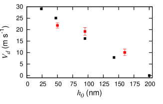
Figure 9: Droplet detachment velocity $V_{d}$ for liquefied triangular Au nanostructures with a side length of $405$ nm and various thicknesses, numerical results ($\blacksquare$) and experimental measurements ($\blacksquare$). Numerical results are obtained using the slip length of $3$ nm.

References

- Maier (2007) S. Maier, Plasmonics: Fundamentals and Applications (Springer-Verlag, New York, 2007).
- Atwater and Polman (2010) H. Atwater and A. Polman, Nat. Mat. 9, 9 (2010).
- Baderi (2006) S. Baderi, Rev. Mod. Phys. 78, 1 (2006).
- Maier et al. (2003) S. A. Maier et al., Nat. Mat. 2, 229 (2003); S. Sun et al., Science 287, 1989 (2000).
- Oron et al. (1997) A. Oron, S. H. Davis, and S. G. Bankoff, Rev. Mod. Phys. 69, 931 (1997); R. Craster and O. Matar, Rev. Mod. Phys. 81, 1131 (2009).
- Habenicht et al. (2005) A. Habenicht et al., Science 309, 2043 (2005).
- Burton et al. (2004) J. C. Burton, J. E. Rutledge, and P. Taborek, Phys. Rev. Lett. 92, 244505 (2004).
- Fuentes-Cabrera et al. (2011) M. Fuentes-Cabrera et al., Phys. Rev. E 83, 041603 (2011).
- Sussman (2003) M. Sussman, J. Comput. Phys 187, 110 (2003); S. Afkhami and M. Bussmann, Int. J. Numer. Meth. Fluids 57, 453 (2008); S. Afkhami and M. Bussmann, Int. J. Numer. Meth. Fluids 61, 827 (2009).
- Bonn et al. (2009) D. Bonn et al., Rev. Mod. Phys. 81, 739 (2009).
- Haley and Miksis (1991) P. J. Haley and M. J. Miksis, J. Fluid Mech. 223, 57 (1991).
- (12) See Supplemental Material including animations at [URL will be inserted by publisher].
- Qian et al. (2004) T. Qian, X.-P. Wang, and P. Sheng, Phys. Rev. Lett. 93, 094501 (2004).
- Popinet (2003) S. Popinet, J. Comput. Phys. 190, 572 (2003).
- Afkhami et al. (2009) S. Afkhami, S. Zaleski, and M. Bussmann, J. Comput. Phys. 228, 5370 (2009).
- Kondic et al. (2009) L. Kondic et al., Phys. Rev. E 79, 026302 (2009); J. D. Fowlkes et al., Nano Lett. 11, 2478 (2011).
- Kim and Chun (2001) H.-Y. Kim and J.-H. Chun, Phys. Fluids 13, 643 (2001); P. Attané, F. Girard, and V. Morin, Phys. Fluids 19, 012101 (2007).
- Young (1805) T. Young, Philos. Trans. R. Soc. London 95 (1805).

References

- Hirt and Nichols (1981) C. W. Hirt and B. D. Nichols, J. Comput. Phys. 39, 201 (1981).
- Gueyffier et al. (1999) D. Gueyffier, J. Li, A. Nadim, R. Scardovelli, and S. Zaleski, J. Comput. Phys. 152, 423 (1999).
- Afkhami and Bussmann (2009) S. Afkhami and M. Bussmann, Int. J. Numer. Meth. Fluids 61, 827 (2009).
- Brackbill et al. (1992) J. U. Brackbill, D. B. Kothe, and C. Zemach, J. Comput. Phys. 100, 335 (1992).
- Sussman (2003) M. Sussman, J. Comput. Phys 187, 110 (2003).
- Cummins et al. (2005) S. J. Cummins, M. M. Francois, and D. B. Kothe, Comp. Struct. 83, 425 (2005).
- Afkhami and Bussmann (2008) S. Afkhami and M. Bussmann, Int. J. Numer. Meth. Fluids 57, 453 (2008).
- Francois et al. (2006) M. M. Francois, S. J. Cummins, E. D. Dendy, D. B. Kothe, J. M. Sicilian, and M. W. Williams, J. Comput. Phys. 213, 141 (2006).
- Haley and Miksis (1991) P. J. Haley and M. J. Miksis, J. Fluid Mech. 223, 57 (1991).
- Young (1805) T. Young, Philos. Trans. R. Soc. London 95 (1805).
- Kim and Chun (2001) H.-Y. Kim and J.-H. Chun, Phys. Fluids 13, 643 (2001).
- Attané et al. (2007) P. Attané, F. Girard, and V. Morin, Phys. Fluids 19, 012101 (2007).
- Fuentes-Cabrera et al. (2011) M. Fuentes-Cabrera, B. Rhodes, M. Baskes, H. Terrones, J. Fowlkes, M. Simpson, and P. Rack, ACS Nano 5, 7130 (2011).
- Habenicht et al. (2005) A. Habenicht, M. Olapinski, F. Burmeister, P. Leiderer, and J. Boneberg, Science 309, 2043 (2005).