Surveillance of the Incidence of Noncommunicable Diseases (NCDs) with Prevalence Data:
Theory and Application to Diabetes in Denmark

Abstract

Secular trends of the incidence of NCDs are especially important as they indicate changes of the risk profile of a population. The article describes a method for detecting secular trends in the incidence from a series of prevalence data - without requiring costly follow-up studies or running a register. After describing the theory, the method is applied to the incidence of diabetes in Denmark.

1 Introduction

Setting up health information systems to monitor the evolving burden of noncommunicable diseases (NCDs) and their risk factors, is one of the claims of the Moscow Declaration, which was approved by the First Global Ministerial Conference on Healthy Lifestyles and NCD control [4]. In that respect, secular trends of the incidence of NCDs are especially important as they indicate changes of the risk profile of the population under consideration. Common ways to detect secular trends in the incidence are either performing a series of follow-up studies or running a register. Both approaches may be very costly and lead to a variety of practical problems. In contrast, a series of prevalence studies sometimes is much easier to accomplish. Based on illness-death model (IDM), this article describes a method for detecting trends in the incidence of NCDs without a series of follow-up studies and without a register.

The next section introduces the IDM and derives the theoretical background for the method. In the third section, the theory is applied to data from the National Diabetes Register in Denmark. The register observed an increasing diabetes incidence in 1995–2004. We show that the trend is detectable using the IDM and a series of prevalence data. The last section contains a summary.

2 Illness-Death Model

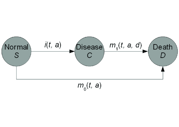
In modelling chronic (i.e., irreversible) diseases, often the three-state model (compartment model) in Figure 1 is used. The numbers of persons in the states Normal and Disease are denoted by $S$ and $C$. The transition intensities (synonymously: rates) between the states are: the incidence rate $i$ and the mortality rates $m_{0}$ and $m_{1}$ of the healthy or the diseased, respectively. These rates generally depend on the calendar time $t$, the age $a$ and in the case of the mortality $m_{1}$ also on the duration of the disease $d$.

Figure 1: Chronic disease model with three states and the corresponding transition rates. People in the state Normal are healthy with respect to the disease under consideration. At onset of the disease, they change to state Disease.

Although the inclusion of the disease duration $d$ is also possible, hereinafter it is assumed that $m_{1}$ does not depend on $d.$ This article analytically describes the relationship between the prevalence of a chronic disease, the incidence and mortality rates. This problem has existed at least since 1934 [5], but so far has only been solved in special cases. The article [3] presents a brief review and further references.

As in [1], we look for the numbers $S(t,a)$ and $C(t,a)$ of healthy and diseased persons in terms of differential equations, which can be derived from the disease model in Figure 1. For the healthy persons we get the following initial value problem:

(1) $$(\partial_{t}+\partial_{a})\,S =-\left[m_{0}+i\right]\,S$$

$$S(t-a,0) =S_{0}(t-a).$$

Here $S_{0}(t-a)=S(t-a,0)$ is the number of (healthy) newborns at calendar time $t-a.$ The notation $\partial_{x}$ denotes the partial derivative with respect to $x,~{}x\in\{t,a\}$. The solution $S(t,a)$ is

(2) $$S(t,a)=S_{0}(t-a)\,\exp\left(-\int_{0}^{a}m_{0}(t-a+\tau,\tau)+i(t-a+\tau,\tau)\,\mathrm{d}\tau\right),$$

which may be checked easily.

The number $C$ of diseased persons are described similarly:

(3) $$(\partial_{t}+\partial_{a})\,C =-m_{1}\,C+i\,S$$

$$C(t,0) =0.$$

The solution is

(4) $$C(t,a)=\int_{0}^{a}i(t-\delta,a-\delta)\,S(t-\delta,a-\delta)\exp\left(-\int_{0}^{\delta}m_{1}(t-\delta+\tau,a-\delta+\tau)\mathrm{d}\tau\right)\mathrm{d}\delta.$$

Equation (4) allows the following interpretation: Starting from $(t,a)$ at $\delta$ time units before, i.e., at $(t-\delta,a-\delta)$, exactly $i(t-\delta,a-\delta)\,S(t-\delta,a-\delta)$ persons newly enter state Disease. Until $(t,a)$ the proportion

$$\exp\left(-\int_{0}^{\delta}m_{1}(t-\delta+\tau,a-\delta+\tau)\mathrm{d}\tau\right)$$

of those has survived. Integration over all possible $0\leq\delta\leq a$ yields the number of diseased persons at time $(t,a).$ After applying the quotient rule to the age-specific prevalence

$$p(t,a)=\frac{C(t,a)}{S(t,a)+C(t,a)}$$

and using (1) and (3) it follows

(5) $$(\partial_{t}+\partial_{a})\,p =\left(1-p\right)\,\left(i-p\,\left(m_{1}-m_{0}\right)\right)$$

$$p(t,0) =0.$$

Remark 1.

For $t,a\geq 0$ with $p(t,a)\neq 1$ it holds

(6) $$i(t,a)=\frac{(\partial_{t}+\partial_{a})\,p(t,a)}{1-p(t,a)}+p(t,a)\,\left(m_{1}(t,a)-m_{0}(t,a)\right).$$

Furthermore, the solution of (5) can be calculated directly via (2) and (4):

(7) $$p(t,a)=\frac{\int\limits_{0}^{a}i(t-\delta,a-\delta)\,\exp\left(-\int\limits_{0}^{\delta}\Psi(t-\delta+\tau,a-\delta+\tau)\mathrm{d}\tau\right)\mathrm{d}\delta}{1+\int\limits_{0}^{a}i(t-\delta,a-\delta)\,\exp\left(-\int\limits_{0}^{\delta}\Psi(t-\delta+\tau,a-\delta+\tau)\mathrm{d}\tau\right)\mathrm{d}\delta},$$

with $\Psi:=m_{1}-m_{0}-i.$

This follows from

$$C(t,a) =\int_{0}^{a}i(t-\delta,a-\delta)\,S_{0}(t-a)$$

$$\qquad\cdot\exp\left(-\int_{0}^{\delta}m_{1}(t-\delta+\tau,a-\delta+\tau)\mathrm{d}\tau-\int_{0}^{a-\delta}(m_{0}+i)(t-a+\tau,\tau)\mathrm{d}\tau\right)\mathrm{d}\delta$$

$$=\int_{0}^{a}i(t-\delta,a-\delta)\,S_{0}(t-a)$$

$$\qquad\cdot\exp\left(-\int_{0}^{\delta}m_{1}(t-\delta+\tau,a-\delta+\tau)\mathrm{d}\tau-\int_{0}^{a}(m_{0}+i)(t-a+\tau,\tau)\mathrm{d}\tau\right.$$

$$\qquad\qquad\qquad+\left.\int_{a-\delta}^{a}(m_{0}+i)(t-a+\tau,\tau)\mathrm{d}\tau\right)\mathrm{d}\delta$$

$$=S_{0}(t-a)\,\exp\left(-\int_{0}^{a}(m_{0}+i)(t-a+\tau,\tau)\mathrm{d}\tau\right)$$

$$\qquad\cdot\int\limits_{0}^{a}i(t-\delta,a-\delta)\,\exp\left(-\int\limits_{0}^{\delta}\Psi(t-\delta+\tau,a-\delta+\tau)\mathrm{d}\tau\right)\mathrm{d}\delta.$$

The first part of the last expression equals $S(t,a)$ and Equation (7) follows.

The usefulness of equation (7) is obvious: Given the incidence $i(t,a)$ and mortalities $m_{0}(t,a),~{}m_{1}(t,a)$, the prevalence $p(t,a)$ can be calculated for all $t,a\geq 0$.

So we can state

Remark 2.

The prevalence $p(t,a)$ is independent from the number $S_{0}$ of newborns.

Remark 3.

For $t,a\geq 0$ it holds: $0\leq p(t,a)\leq 1.$

Remark 4.

If for some $(t_{1},a_{1})$ the integral

$$\Upsilon(t_{1},a_{1}):=\int\limits_{0}^{a_{1}}i(t_{1}-\delta,a_{1}-\delta)\,\exp\left(-\int\limits_{0}^{\delta}\Psi(t_{1}-\delta+\tau,a_{1}-\delta+\tau)\mathrm{d}\tau\right)\mathrm{d}\delta$$

is lower than for $(t_{2},a_{2}):~{}\Upsilon(t_{1},a_{1})<\Upsilon(t_{2},a_{2})$, then it holds $p(t_{1},a_{1})<p(t_{2},a_{2}).$ This follows from observing that $x\mapsto\nicefrac{{x}}{{1+x}},~{}x\geq 0$ is strictly increasing.

At the end of the section we introduce the relative mortality $R(t,a).$ For $(t,a)\geq 0$ with $m_{0}(t,a)>0,$ define

$$R(t,a)=\frac{m_{1}(t,a)}{m_{0}(t,a)}.$$

Now we have all the definitions and results for the next section.

3 Diabetes in Denmark

In the article [2] the age-specific prevalence of diabetes for men (and women) in Denmark in the period 1995-2007 is presented in great detail. The results are based on a complete survey of the Danish population ($n>5$ million). Classifying a person as diabetic is done by combining different health registers, which yields a sensitivity of more than 85% [2, p. 2188]. In this paper we confine ourselves to the male population in Denmark. The age-specific incidence rate $i$ for 2004 is given for all age groups, but for the other years in the period 1995-2007 just relatively to 2004, averaged across all age groups; likewise, with the mortality $m_{0}$ of the non-diabetic population. Mortality $m_{1}$ significantly depends on the disease duration [2, Fig. 4]. To the apply the model of the previous section model, the duration dependence has to be suppressed. This is done by an initialization step: The relative mortality $R^{\star}(a)$ is calculated such that the observed incidence and the associated increase in prevalence from 1995 to 1996 are in agreement. Therefor, the Equation (5) is solved for $m_{1}$. Then, $R^{\star}$ is calculated by $R^{\star}=\nicefrac{{m_{1}}}{{m_{0}}}.$ For the period 1996 - 2004, this relative mortality is kept fixed and Equation (5) is solved for $i$ as in Remark 1 with $m_{1}=R^{\star}\,m_{0}.$ By doing so, the relative mortality $R^{\star}$ for the period 1996-2004 is assumed to be independent from calendar time. Thus, we have a two-step approach:

1. Initialization: Calculate $R^{\star}$ by fitting the observed incidence rate in 1995 and the increase in age-specific prevalence from 1995 to 1996.

2. Application: Derivation of the incidence rates in 1996-2004 via Remark 1 mit $m_{1}(t,a)=R^{\star}(a)\,m_{0}(t,a).$

Remark 5.

After initialization, we just use the mortality $m_{0}$ of the non-diabetic population and the prevalences $p(t,a),$ $t=1996,\dots,2004,$ for deriving $i(t,a),$ $t=1996,\dots,2004.$

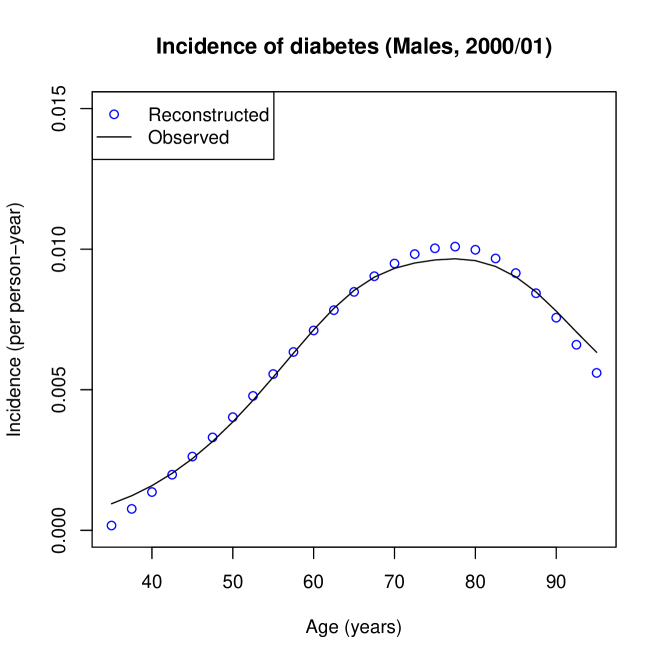
Figure 2 shows the results of applying the model to 2001 (circles). For comparison the observed incidence is shown (solid line). Obviously, the data are in good agreement.

Figure 2: Age-spefic incidence rate in 2001: observed (solid line) and reconstructed by the model (circles).

Now, the increase in the incidence can be examined. For some of the age groups, the incidence rate over calendar time is shown in Figure 3. In addition, the regression lines and the corresponding correlation coefficients $r$ are given. In all age groups there is a significant upward trend. The higher the age, the better the fit of the linear regression model. Table 1 shows the numerical values for all age groups.

Figure 3: Incidence rates over calendar time for some age groups.

Age-	Annual	Correlation-
group	increase (%)	coefficient
40 – 44	9.2	0.76
45 – 49	9.6	0.86
50 – 54	9.3	0.90
55 – 59	8.8	0.93
60 – 64	8.3	0.96
65 – 69	8.0	0.98
70 – 74	7.8	0.99
75 – 79	7.9	0.99
80 – 84	8.2	0.99

Table 1: Parameters of the secular trends in the incidence rates in the age groups.

The annual increase rates in the age groups (second column in Table 1) are all greater than the corresponding value 5.3% reported in [2, p. 2190]. However, the reported increase of 5.3% refers to all persons (both sexes, all age groups). Hence, a direct comparison with the values of Table 1 is impossible.

4 Summary

In this work, a novel method for deriving trends in incidence from a sequence of prevalence studies is presented. With a view to the tremendous effort required by collecting incidence data, the novel method provides a simpler alternative. A typical application is the conversion of a sequence of telephone surveys for the collection of age-specific prevalence of a chronic disease into a sequence of incidence data.

As a first application, the method was used with data from the Danish National Diabetes Register. The directly observed secular trend in the incidence is visible by the new method as well.

In the application to the Danish Diabetes Register, the relative mortality $R^{\star}$ in 1995 has been extrapolated for the period 1996-2004. While this may be possible for a period of eight years is a word of caution is in order:

Remark 6.

The calendar time trend in mortality $m_{0}$ of the non-diabetic population is usually much better known than the trend in mortality $m_{1}$ of the patients. The reason is that $m_{0}$ is surveyed on a demographic scale, while $m_{1}$ is investigated sporadically in epidemiological studies only. In epidemiology, one might try to link the time trend in $m_{1}$ to the time trend in $m_{0}$. The idea might be to measure a relative mortality $R$ at some time $t^{\prime}<t$ and extrapolate from $t^{\prime}$ to $t$ and set $m_{1}(t,a)=R(t^{\prime},a)\,m_{0}(t,a).$ Indeed, time dependence of $m_{1}$ is enforced, but this approach may lead to a possibly unexpected increase in the prevalence. If the incidence $i$ is independent of $t$ and the family of functions $t\mapsto m_{0,a}(t):=m_{0}(t,a)$ is decreasing for all $a\geq 0$, then, by Remark 4, the function $t\mapsto p_{a}(t):=p(t,a)$ is monotonically increasing for all $a\geq 0.$ This means: although the incidence $i$ is remains unchanged by the calendar time, by increasing the life expectancy of the healthy (decreasing $m_{0,a}$), the prevalence increases. Extrapolating the relative mortality $R$ from $t^{\prime}$ to $t$ therefore must be viewed critically.

Beside the presentation of the theoretical background, this work is little more than a feasibility study. There are two sources of limitations:

1. Data: Due to the incomplete detection of diabetes cases and the shortened report of incidence trends (pooled for all persons), a direct comparison between the observed and derived trends in the incidence is impossible.

2. Model: Although it is evident that $m_{1}$ depends on the duration $d$ of diabetes, this dependency is neglected. In additon, the relative mortality $R^{\star}$ has been calculated for 1995, but has been extrapolated to 1996-2004.

Both inaccuracies interact, which makes a rigorous evaluation difficult. Thus, a systematic evaluation of the method based on a comprehensive simulation study is necessary.

Contact:
Ralph Brinks
German Diabetes Center
Auf’m Hennekamp 65
D- 40225 Duesseldorf
ralph.brinks@ddz.uni-duesseldorf.de