Dynamical influence processes on networks:
General theory and applications to social contagion

Abstract

We study binary state dynamics on a network where each node acts in response to the average state of its neighborhood. Allowing varying amounts of stochasticity in both the network and node responses, we find different outcomes in random and deterministic versions of the model. In the limit of a large, dense network, however, we show that these dynamics coincide. We construct a general mean field theory for random networks and show this predicts that the dynamics on the network are a smoothed version of the average response function dynamics. Thus, the behavior of the system can range from steady state to chaotic depending on the response functions, network connectivity, and update synchronicity. As a specific example, we model the competing tendencies of imitation and non-conformity by incorporating an off-threshold into standard threshold models of social contagion. In this way we attempt to capture important aspects of fashions and societal trends. We compare our theory to extensive simulations of this “limited imitation contagion” model on Poisson random graphs, finding agreement between the mean-field theory and stochastic simulations.

I Introduction

Networks continue to be an exploding area of research due to their generality and ubiquity in physical, biological, technological, and social settings. Dynamical processes taking place on networks are now recognized as the most natural description for a number of phenomena. These include neuron behavior in the brain (Coombes et al., 2006), cellular genetic regulation (Milo et al., 2002), ecosystem dynamics and stability (Bascompte, 2009), and infectious diseases (Rohani et al., 2010). This last category, the study of biological contagion, is in many ways similar to social contagion, which refers to the spreading of ideas, fashions, or behaviors among people (Ugander et al., 2012; Centola, 2010). This concept underlies the vastly important contemporary area of viral marketing, driven by the ease with which media can be shared and spread through social network websites.

In this work, we present results for a very general model of networked map dynamics, motivated by models of social contagion. We will describe our model in a social context, but it is more general since it is a type of boolean network (Aldana et al., 2003). These are closely related to physical models of percolation (Stauffer and Aharony, 1994) and magnetism (Newman, 2003; Aldana et al., 2003), and they have been employed in a number of fields such as computational neuroscience (Schneidman et al., 2006), ecology (Campbell et al., 2011), and others. Nodes, which in our case represent people, are allowed two possible states. These could encode rioting or not rioting (Granovetter, 1978), buying a particular style of tie (Granovetter and Soong, 1986), liking a band or style of music, or taking a side in a debate (Galam, 2008). Each node has a response function, a map which determines the state the node will take in response to the average state of nodes in its neighborhood. The model can thus represent many behaviors, as long as there are only two mutually exclusive possibilities, where agents make a choice based on the average of their neighbors’ choices. Schelling (1971, 1973) and Granovetter (1978) pioneered the use of threshold response functions in such models of collective social behavior. This was based on the intuition that, for a person to adopt some new behavior, the fraction of the population exhibiting it might need to exceed some critical value, the person’s threshold. These threshold social contagion models, which are a subclass of our general model, have already been studied on networks (Watts, 2002; Dodds and Watts, 2004).

In our theoretical analysis, we focus on the derivation and analysis of dynamical master equations that describe the expected evolution of the system state in the general influence process model. These master equations are given in both exact form and mean-field approximations. We also show how certain dense network limits lead to the convergence of the dynamics to the average response function map dynamics.

We then apply the general theory to a particular limited imitation contagion model (Dodds et al., 2013). Nodes act according to competing tendencies of imitation and non-conformity. One can argue that these two ingredients are essential to all trends; indeed, Simmel, in his classic essay “Fashion” (1957), believed that these are the main forces behind the creation and destruction of fashions. Our model is not meant to be quantitative, except perhaps in carefully designed experiments. Nodes in the model lack memory of their past states, which is likely an important effect in the adoption of real fashions. It does capture qualitative features with which we are familiar: some trends take off and some do not, and some trends are stable while others vary wildly through time.

In Section II, we define the general model and its deterministic and stochastic variants. In Section III, we provide an analysis of the model when the underlying network is fixed. In Section IV, we develop a mean-field theory of the model on generalized random networks. In Section V, we consider the model on Poisson random networks with a specific kind of response function that reflects the limited imitation we expect in many social contagion processes. For this specific case, we compare the results of simulations and theory. Finally, in Section VI, we present conclusions and directions for further research.

II General model

Let $\mathscr{G}=(V,E)$ be a network with $N=|V|$ nodes, where $V$ is the node set and $E$ is the edge set. We let $A=A(\mathscr{G})$ denote the adjacency matrix; entry $A_{ij}$ is the number of edges from node $j$ to node $i$. Assign each node $i\in V$ a response function $f_{i}:[0,1]\to\{0,1\}$, and let $\mathbf{x}(0)\in\{0,1\}^{N}$ be the vector of initial node states. At time step $t$, each node $i$ computes the fraction

$$\phi_{i}(t)=\frac{\sum_{j=1}^{N}A_{ij}x_{j}(t)}{\sum_{j=1}^{N}A_{ij}}$$ (1)

of their neighbors in $\mathscr{G}$ who are active and takes the state

$$x_{i}(t+1)=f_{i}\left(\phi_{i}(t)\right)$$ (2)

at the next time step.

The above defines a deterministic dynamical system given a network and set of response functions. We call this a realization of the model (Aldana et al., 2003). Each node is in either the 0 or 1 state; we refer to these as the off/inactive and on/active states, respectively. In the context of contagion, these would be the susceptible and infected states. With these binary states, our model is a particular kind of Boolean network. These exhibit rich dynamics and have a long history in the literature. Unfamiliar readers should consult the review by Aldana et al. (2003) and references therein. Note that each node reacts only to the fraction of its neighbors who are active, rather than the absolute number, and the identities of the input nodes do not matter. Each node’s input varies from 0 to 1 in steps of $1/k_{i}$, where $k_{i}=\sum_{j=1}^{N}A_{ij}$ is node $i$’s degree (in-degree if $\mathscr{G}$ is not a simple graph).

The behavior of the model depends strongly on the response functions $f_{i}$. Leaving these undetermined, the principle feature of the model is its neighborhood-averaging property. Because of local averaging, one might expect that the dynamics of the network global average activity might be close to the map dynamics of the average of the $f_{i}$. We show this is the case in dense enough networks in Sections III.2 and IV.2. This averaging property also introduces an invariance to the number of inputs a given node receives.

In the rest of this Section, we will describe some variations of the basic model which also differentiate our model from the Boolean networks extant in the literature. This is mainly due to the response functions, but also the type of random network on which the dynamics take place, varying amounts of stochasticity introduced into the networks and response functions, and the possibility of asynchronous updates.

II.1 The networks considered

The mean-field analysis in Section IV is applicable to any network which can be characterized by its degree distribution. The vast majority of the theory of random Boolean networks considers only regular random networks. Fortunately, such theories are easily generalized to other types of networks with independently chosen edges, such as Poisson (Erdös-Rényi) and configuration model random networks (Newman, 2003; Bollobás, 2001). We develop specific results for Poisson random networks, and these are the networks used for the example problem in Section V.

II.2 Stochastic variants

The specific network and response functions determine exactly which behaviors are possible. These are chosen from some distribution of networks, such as $\mathcal{G}(N,k_{\rm avg}/N)$ (Poisson random networks on $N$ nodes with edge probability $k_{\rm avg}/N$), and some distribution of response functions. In the example of Section V, the response functions are parameterized solely by two thresholds, $\phi_{{\rm on}}$ and $\phi_{{\rm off}}$, so the distribution of response functions is determined by the joint density $P(\phi_{{\rm on}},\phi_{{\rm off}})$. Again, the specific network and response functions define a realization of the model. When these are fixed for all time, we have, in principle, full knowledge of the possible model dynamics. Given an initial condition $\mathbf{x}(0)$, the dynamics $\mathbf{x}(t)$ are deterministic and known for all $t\geq 0$. As for all finite Boolean networks, the system dynamics are eventually periodic, since the state space $\{0,1\}^{N}$ is finite (Aldana et al., 2003).

We allow for randomness in two parts of the model: the network and response functions. The network and responses are each either fixed for all time or resampled each time step. Taking all possible combinations yields four different designs (see Table 1). If the dynamics are stochastic in any way, the system is no longer eventually periodic. Fluctuations at the node level enable a greater exploration of state space, and the behavior is comparable to that of the general class of discrete-time maps. Roughly speaking, the mean-field theory we develop in Section IV becomes more accurate as we introduce more stochasticity.

In this paper, the network and response functions are either fixed for all time or resampled every time step. One could tune smoothly between the two extremes by introducing rates at which these reconfigurations occur. These rates are inversely related to quantities that behave like temperature, one for the network and another for the response functions. Holding a quantity fixed corresponds to zero temperature, since there are no fluctuations. Any randomness is quenched. The stochastic and rewired cases correspond to high or infinite temperature, because reconfigurations occur every time step. This is an annealed version of the model.

	Rewiring network	Fixed network
Probabilistic response	P-R	P-F
Deterministic response	D-R	D-F

Table 1: The four different ways we implement the model, corresponding to differing amounts of quenched randomness. These are the combinations of fixed or rewired networks and probabilistic or deterministic response functions. In the thermodynamic limit of the rewired versions, where the network and response functions change every time step, the mean-field theory (Sec. IV) is exact.

II.2.1 Rewired networks

First, the network itself can change every time step. This is the rewiring (R), as opposed to fixed (F), network case. For example, we could draw a new network from $\mathcal{G}(N,k_{\rm avg}/N)$ every time step. This amounts to rewiring the links while keeping the degree distribution fixed, and it is alternately known as a mean field, annealed, or random mixing variant as opposed to a fixed network or quenched model (Aldana et al., 2003).

II.2.2 Probabilistic responses

Second, the response functions can change every time step. This is the probabilistic (P), as opposed to the deterministic (D), response function case. For our social contagion example, there needs to be a well-defined distribution $P(\phi_{{\rm on}},\phi_{{\rm off}})$ for the thresholds. For large $N$, this amounts to having a single response function, the expected response function

$$\bar{f}(\phi)=\int\mbox{d}\phi_{{\rm on}}\int\mbox{d}\phi_{{\rm off}}\;P(\phi_{{\rm on}},\phi_{{\rm off}})f(\phi;\phi_{{\rm on}},\phi_{{\rm off}}).$$ (3)

We call $\bar{f}:[0,1]\to[0,1]$ the probabilistic response function. Its interpretation is the following. For an updating node with a fraction $\phi$ of active neighbors at the current time step, then, at the next time step, the node assumes the active state with probability $\bar{f}(\phi)$ and the inactive state with probability $1-\bar{f}(\phi)$.

II.3 Update synchronicity

Finally, we introduce a parameter $\alpha$ for the probability that a given node updates. When $\alpha=1$, all nodes update each time step, and the update rule is said to be synchronous. When $\alpha\approx 1/N$, only one node is expected to update with each time step, and the update rule is said to be effectively asynchronous. This is equivalent to a randomly ordered sequential update. For intermediate values, $\alpha$ is the expected fraction of nodes which update each time step.

III Fixed networks

Consider the case where the response functions and network are fixed (D-F), but the update may be synchronous or asynchronous. Extend the definition of $x_{i}(t)$ to now be the probability that node $i$ is in the active state at time $t$. Note that this agrees with our previous definition as the state of node $i$ when $x_{i}(t)=0$ or 1. Then the $x_{i}$ follow the master equation

$$x_{i}(t+1)=\alpha f_{i}\left(\frac{\sum_{j=1}^{N}A_{ij}x_{j}(t)}{\sum_{j=1}^{N}A_{ij}}\right)+(1-\alpha)x_{i}(t),$$ (4)

which can be written in matrix-vector notation as

$$\mathbf{x}(t+1)=\alpha\,\mathbf{f}\left(T\mathbf{x}(t)\right)+(1-\alpha)\mathbf{x}(t).$$ (5)

Here $T=D^{-1}A$ is sometimes called the transition probability matrix (since it also occurs in the context of a random walker), $D=\text{diag}(k_{i})$ is the diagonal degree matrix, and $\mathbf{f}=(f_{i})$ . If $\alpha=1$, then $\mathbf{x}(t)\in\{0,1\}^{N}$ and we recover the fully deterministic response function dynamics given by (1) and (2).

III.1 Asynchronous limit

Here, we show that when $\alpha\approx 1/N$, time is effectively continuous and the dynamics can be described by an ordinary differential equation. This is similar to the analysis of Gleeson (2008). Consider Eqn. (5). Subtracting $\mathbf{x}(t)$ from both sides and setting $\Delta\mathbf{x}(t)=\mathbf{x}(t+1)-\mathbf{x}(t)$ and $\Delta t=1$ yields

$$\frac{\Delta\mathbf{x}(t)}{\Delta t}=\alpha\left(\mathbf{f}(T\mathbf{x}(t))-\mathbf{x}(t)\right).$$ (6)

Since $\alpha$ is assumed small, the right hand side is small, and thus $\Delta\mathbf{x}(t)$ is also small. Making the continuum approximation $\mbox{d}\mathbf{x}(t)/\mbox{d}t\approx\Delta\mathbf{x}(t)/\Delta t$ yields the differential equation

$$\frac{\mbox{d}\mathbf{x}}{\mbox{d}t}=\alpha\left(\mathbf{f}(T\mathbf{x})-\mathbf{x}\right).$$ (7)

The parameter $\alpha$ sets the time scale for the system. Below we see that, from their form, similar asynchronous, continuous time limits apply to the dynamical equations in the densely connected case, Eqn. (8), and in the mean-field theory, Eqns. (11) and (12).

III.2 Dense network limit for Poisson random networks

Mathematical random graph and random matrix theories often deal with condensation results, where quantities of interest, such as adjacency matrices, become overwhelmingly concentrated around some typical value in a limit. These limits are dense in the sense that $k_{\rm avg}\to\infty$ in the thermodynamic limit $N\to\infty$. The mean field theory of Section IV applies to sparse graphs, which have finite $k_{\rm avg}$ in the thermodynamic limit. The following result is particular to Poisson random networks, however, similar results should hold for other random networks with corresponding dense limits.

Define the normalized Laplacian matrix as $\mathcal{L}\equiv I-D^{-1/2}AD^{-1/2}$, where $I$ is the identity (West, 2001). So $T=D^{-1/2}(I-\mathcal{L})D^{1/2}$. Let $\mathbf{1}_{N}$ denote the length-$N$ column vector of ones. Oliveira (2010) has shown that when $k_{\rm avg}$ grows at least as fast as $\log N$, there exists a typical normalized Laplacian matrix $\mathcal{L}^{\text{typ}}=I-\mathbf{1}_{N}\mathbf{1}_{N}^{T}/N$ such that the actual $\mathcal{L}\approx\mathcal{L}^{\text{typ}}$. In this limit, the degrees should also be approximately uniform, $k_{i}\approx k_{\rm avg}$ for all $i\in V$, since the coefficient of variation of degrees vanishes in the Poisson model as $k_{\rm avg}\to\infty$.

If we use the approximations $\mathcal{L}\approx\mathcal{L}^{\text{typ}}$ and $D\approx\text{diag}\,(k_{\rm avg})$, then $T\approx T^{\text{typ}}=\mathbf{1}_{N}\mathbf{1}_{N}^{T}/N$. Since

$$T^{\text{typ}}\mathbf{x}(t)=\sum_{i=1}^{N}x_{i}(t)/N\equiv\phi(t),$$

$T^{\text{typ}}$ operating on the state gives the network average activity, denoted $\phi$ without any subscript. Using the previous approximations in Eqn. (5) and averaging over all nodes, we find

$$\phi(t+1)=\alpha\bar{f}(\phi(t))+(1-\alpha)\phi(t)\equiv\Phi(\phi(t);\alpha)$$ (8)

in the large $N$ limit. This requires the average of nodes’ individual response functions $\sum_{i=1}^{N}f_{i}/N$ to converge in a suitable sense to the probabilistic response function $\bar{f}$, Eqn. (3). Note that $\alpha$ tunes between the probabilistic response function $\Phi(\phi;1)=\bar{f}(\phi)$ and the line $\Phi(\phi;0)=\phi$. Also, the fixed points of $\Phi$ are fixed points of $\bar{f}$, but their stability will depend on $\alpha$.

We conclude that when the network is dense, it ceases to affect the dynamics, since each node sees a large number of other nodes. The network is effectively the complete graph. In this way we recover the map models of Granovetter and Soong (1986), which are derived for a well-mixed population.

IV Mean-field theory

Making a mean-field calculation refers to replacing the complicated interactions among many particles by a single interaction with some effective external field. There are analogous techniques for understanding network dynamics. Instead of considering the $|E|$ interactions among the $N$ nodes, network mean-field theories derive self-consistent expressions for the overall behavior of the network after averaging over large sets of nodes. These have been fruitful in the study of random Boolean networks (Derrida and Pomeau, 1986) and can work well when networks are non-random (Melnik et al., 2011).

We derive a mean-field theory, in the thermodynamic limit, for the dynamics of the general model by blocking nodes according to their degree class. This is equivalent to nodes retaining their degree but rewiring edges every time step. The model is then part of the well-known class of random mixing models with non-uniform contact rates. Probabilistic (P-R) and deterministic (D-R) response functions result in equivalent behavior for these random mixing models. The important state variables end up being the active density of stubs, i.e. half-edges or node-edge pairs. In an undirected network without degree-degree correlations, the state is described by a single variable $\rho(t)$. In the presence of correlations we must introduce more variables $\left\{\rho_{k}(t)\right\}$ to deal with the relevant degree classes.

IV.1 Undirected networks

To derive the mean-field equations in the simplest case—undirected, uncorrelated random networks—consider a degree $k$ node at time $t$. The mean-field hypothesis states that the probability a given stub is active is uniform across all nodes and equal to $\rho$. Then the probability that an average node is in the active state at time $t+1$ given a density $\rho$ of active stubs is

$$F_{k}(\rho;\bar{f})=\sum_{j=0}^{k}\binom{k}{j}\rho^{j}\left(1-\rho\right)^{k-j}\bar{f}\left(j/k\right),$$ (9)

where each term in the sum counts the contributions from having $j=0,1,\ldots,k$ active neighbors. The probability of choosing a random stub which ends at a degree $k$ node is $q_{k}=kp_{k}/k_{\rm avg}$ in an uncorrelated random network (Newman, 2003). This is sometimes called the edge-degree distribution. So if all of the nodes update synchronously, the active density of stubs at $t+1$ will be

$$g(\rho;p_{k},\bar{f})=\sum_{k=1}^{\infty}q_{k}F_{k}\left(\rho;\bar{f}\right)=\sum_{k=1}^{\infty}\frac{kp_{k}}{k_{\rm avg}}F_{k}\left(\rho;\bar{f}\right).$$ (10)

Finally, if each node only updates with probability $\alpha$, we have the following map for the density of active stubs:

$$\rho(t+1) =\alpha\,g\left(\rho(t);p_{k},\bar{f}\right)+(1-\alpha)\rho(t)$$ (11)

$$\equiv G\left(\rho(t);p_{k},\bar{f},\alpha\right).$$

By a similar argument, the active density of nodes is given by

$$\phi(t+1) =\alpha\,h\left(\rho(t);p_{k},\bar{f}\right)+\left(1-\alpha\right)\phi(t)$$ (12)

$$\equiv H\left(\rho(t),\phi(t);p_{k},\bar{f},\alpha\right),$$

where

$$h\left(\rho;p_{k},f\right)=\sum_{k=0}^{\infty}p_{k}F_{k}\left(\rho;\bar{f}\right).$$ (13)

Note that the stub or edge-oriented state variable $\rho$ contains all of the dynamically important information, rather than the node-oriented variable $\phi$. This is because nodes can only influence each other through edges, so the number of active edges is a more important measure of the network activity than the number of active nodes. We derived these equations in terms of stubs, meaning that $\rho$ actually keeps track of both the node and edge information. Eqns. (10) and (11) can be interpreted as a branching process for the density of active stubs.

IV.2 Analysis of the map equation and another dense limit

Here we study the properties of the mean field maps $G$ and $H$, Eqns. (11) and (12), which in turn depend on $F_{k}$, Eqn. (9). The function $F_{k}(\rho;\bar{f})$ is known in polynomial approximation theory as the $k$th Bernstein polynomial (in the variable $\rho$) of $\bar{f}$ (Phillips, 2003). Bernstein polynomials have important applications in computer graphics due to their “shape-preserving properties” (Peña, 1999). The Bernstein operator $\mathbb{B}_{k}$ takes $\bar{f}\mapsto F_{k}$. This is a linear, positive operator which preserves convexity for all $k$ and exactly interpolates the endpoints $\bar{f}(0)$ and $\bar{f}(1)$. Immediate consequences include that each $F_{k}$ is a smooth function and the $m$th derivatives $F_{k}^{(m)}(x)\to\bar{f}^{(m)}(x)$ where $\bar{f}^{(m)}(x)$ exists. For $\bar{f}$ concave down, such as the tent or logistic maps, then $F_{k}$ is concave down for all $k$ and $F_{k}$ increases to $\bar{f}$ ($F_{k}\nearrow\bar{f}$) as $k\to\infty$. This convergence is typically slow. Importantly, $F_{k}\nearrow\bar{f}$ implies that $g\left(\rho;p_{k},\bar{f}\right)\leq\bar{f}$ for any degree distribution $p_{k}$.

In some cases, the dynamics of the undirected mean-field theory given by $\rho(t+1)=G\left(\rho(t)\right)$, Eqn. (11), are effectively those of the map $\Phi$, from the dense limit Eqn. (8). We see that $g$, Eqn. (10), can be seen as the expectation of a sequence of random functions $F_{k}$ under the edge-degree distribution $q_{k}$. Indeed, this is how it was derived. From the convergence of the $F_{k}$’s, we expect that $g(\rho;p_{k},\bar{f})\approx\bar{f}(\rho)$ if the average degree $k_{\rm avg}$ is “large enough” and the edge-degree distribution has a “sharp enough” peak about $k_{\rm avg}$ (we will clarify this soon). Then as $k_{\rm avg}\to\infty$, the mean-field coincides with the dense network limit we found for Poisson random networks, Eqn. (8). A sufficient condition for this kind of convergence is the same that we used in justifying the uniform degree approximation in Section III.2: The coefficient of variation of the degree distribution must vanish as $k_{\rm avg}\to\infty$. Equivalently, the standard deviation $\sigma(k_{\rm avg})$ of the degree distribution must be $o(k_{\rm avg})$. In Appendix A we prove this as Lemma 1.

In general, if the original degree distribution $p_{k}$ is characterized by having mean $k_{\rm avg}$, variance $\sigma^{2}$, and skewness $\gamma_{1}$, then the edge-degree distribution $q_{k}$ will have mean $k_{\rm avg}+\sigma^{2}/k_{\rm avg}$ and variance $\sigma^{2}[1+\gamma_{1}\sigma/k_{\rm avg}-(\sigma/k_{\rm avg})^{2}]$. Considering the behavior as $k_{\rm avg}\to\infty$, we can conclude that requiring $\sigma=o(k_{\rm avg})$ and $\gamma_{1}=o(1)$ are sufficient conditions on $p_{k}$ to apply Lemma 1. Poisson degree distributions ($\sigma=\sqrt{k_{\rm avg}}$ and $\gamma_{1}=k_{\rm avg}^{-1/2}$) fit these criteria. Heavy-tailed families of distributions, in general, do not.

The fact that we can take a dense limit in the mean-field model and find the same result using rigorous random matrix theory is worth noting. In general, mean-field models are not rigorously justified. For finite $N$, the quenched dynamics, which we know are deterministic and eventually periodic, are very different from the annealed dynamics, which we will show can be chaotic. The equivalence of the two limits indicates that quenched and annealed dynamics become indistinguishable as $N\to\infty$. We believe that the approach to such a singular limit should reveal interesting discrepancies between the two models.

IV.3 Generalized random networks

In more general random networks, nodes can have both undirected and directed incident edges. We denote node degree by a vector $\mathbf{k}=({k^{\text{(u)}}},{k^{\text{(i)}}},{k^{\text{(o)}}})^{T}$ (for undirected, in-, and out-degree) and write the degree distribution as $p_{\mathbf{k}}\equiv P(\mathbf{k})$. There may also be correlations between node degrees. We encode correlations of this type by the conditional probabilities

$$p^{(\rm u)}_{\mathbf{k},\mathbf{k}^{\prime}}\equiv P(\mathbf{k},\mathrm{undirected}|\mathbf{k}^{\prime})$$

$$p^{(\rm i)}_{\mathbf{k},\mathbf{k}^{\prime}}\equiv P(\mathbf{k},\mathrm{incoming}|\mathbf{k}^{\prime})$$

$$p^{(\rm o)}_{\mathbf{k},\mathbf{k}^{\prime}}\equiv P(\mathbf{k},\mathrm{outgoing}|\mathbf{k}^{\prime}),$$

the probability that an edge starting at a degree $\mathbf{k}^{\prime}$ node ends at a degree $\mathbf{k}$ node and is, respectively, undirected, incoming, or outgoing relative to the destination degree $\mathbf{k}$ node. We introduced this convention in a series of papers (Payne et al., 2011; Dodds et al., 2011). These conditional probabilities can also be defined in terms of the joint distributions of node types connected by undirected and directed edges. We omit a detailed derivation, since it is similar to that in Section IV.1 and similar to the equations for the time evolution of a contagion process (Payne et al., 2011, Eqns. (13–15)) (see also Gleeson and Cahalane, 2007).

The result is a coupled system of equations for the density of active stubs which now may depend on node type ($\mathbf{k}$) and edge type (undirected or directed):

$$\rho_{\mathbf{k}}^{(\rm u)}(t+1) =(1-\alpha)\rho_{\mathbf{k}}^{(\rm u)}(t)+\alpha\sum_{\mathbf{k}^{\prime}}p^{(\rm u)}_{\mathbf{k},\mathbf{k}^{\prime}}\sum_{j_{u}=0}^{{k^{\text{(u)}}}^{\prime}}\sum_{j_{i}=0}^{{k^{\text{(i)}}}^{\prime}}\binom{{k^{\text{(u)}}}^{\prime}}{j_{u}}\binom{{k^{\text{(i)}}}^{\prime}}{j_{i}}$$ (14)

$$\qquad\times\left[\rho_{\mathbf{k}^{\prime}}^{(\rm u)}(t)\right]^{j_{u}}\left[1-\rho_{\mathbf{k}^{\prime}}^{(\rm u)}(t)\right]^{({k^{\text{(u)}}}^{\prime}-j_{u})}\left[\rho_{\mathbf{k}^{\prime}}^{(\rm i)}(t)\right]^{j_{i}}\left[1-\rho_{\mathbf{k}^{\prime}}^{(\rm i)}(t)\right]^{({k^{\text{(i)}}}^{\prime}-j_{i})}$$

$$\qquad\times\bar{f}\left(\frac{j_{u}+j_{i}}{{k^{\text{(u)}}}^{\prime}+{k^{\text{(i)}}}^{\prime}}\right),$$

$$\rho_{\mathbf{k}}^{(\rm i)}(t+1) =(1-\alpha)\rho_{\mathbf{k}}^{(\rm i)}(t)+\alpha\sum_{\mathbf{k}^{\prime}}p^{(\rm i)}_{\mathbf{k},\mathbf{k}^{\prime}}\sum_{j_{u}=0}^{{k^{\text{(u)}}}^{\prime}}\sum_{j_{i}=0}^{{k^{\text{(i)}}}^{\prime}}\binom{{k^{\text{(u)}}}^{\prime}}{j_{u}}\binom{{k^{\text{(i)}}}^{\prime}}{j_{i}}$$ (15)

$$\qquad\times\left[\rho_{\mathbf{k}^{\prime}}^{(\rm u)}(t)\right]^{j_{u}}\left[1-\rho_{\mathbf{k}^{\prime}}^{(\rm u)}(t)\right]^{({k^{\text{(u)}}}^{\prime}-j_{u})}\left[\rho_{\mathbf{k}^{\prime}}^{(\rm i)}(t)\right]^{j_{i}}\left[1-\rho_{\mathbf{k}^{\prime}}^{(\rm i)}(t)\right]^{({k^{\text{(i)}}}^{\prime}-j_{i})}$$

$$\qquad\times\bar{f}\left(\frac{j_{u}+j_{i}}{{k^{\text{(u)}}}^{\prime}+{k^{\text{(i)}}}^{\prime}}\right).$$

The active fraction of nodes at a given time is

$$\phi(t+1) =(1-\alpha)\phi(t)+\alpha\sum_{\mathbf{k}}p_{\mathbf{k}}\sum_{j_{u}=0}^{{k^{\text{(u)}}}}\sum_{j_{i}=0}^{{k^{\text{(i)}}}}\binom{{k^{\text{(u)}}}}{j_{u}}\binom{{k^{\text{(i)}}}}{j_{i}}$$ (16)

$$\qquad\times\left[\rho_{\mathbf{k}}^{(\rm u)}(t)\right]^{j_{u}}\left[1-\rho_{\mathbf{k}}^{(\rm u)}(t)\right]^{({k^{\text{(u)}}}-j_{u})}\left[\rho_{\mathbf{k}}^{(\rm i)}(t)\right]^{j_{i}}\left[1-\rho_{\mathbf{k}}^{(\rm i)}(t)\right]^{({k^{\text{(i)}}}-j_{i})}$$

$$\qquad\times\bar{f}\left(\frac{j_{u}+j_{i}}{{k^{\text{(u)}}}+{k^{\text{(i)}}}}\right).$$

Because these expressions are very similar to the undirected case, we expect similar convergence properties to those in Sec. IV.2. However, an explicit investigation of this convergence is beyond the scope of the current paper.

V Limited imitation contagion model

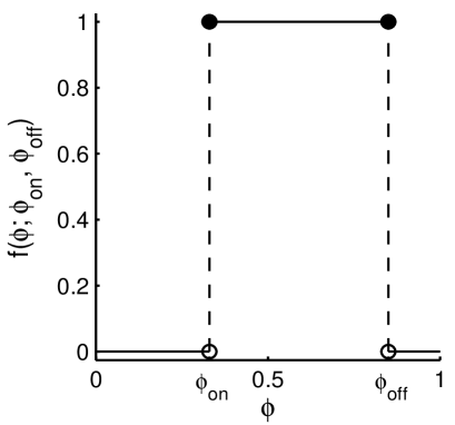
As a motivating example of these networked map dynamics, we study an extension of the classical threshold models of social contagion (such as Schelling, 1971, 1973; Granovetter, 1978; Watts, 2002; Dodds and Watts, 2004, among others). In threshold models, a node becomes active if the active fraction of its friends surpasses its threshold. What differentiates our limited imitation contagion model from the standard models is that the response function includes an off-threshold, above which the node takes the inactive state. We assign each node $i\in V$ an on-threshold $\phi_{{\rm on},i}$ and an off-threshold $\phi_{{\rm off},i}$, requiring $0\leq\phi_{{\rm on},i}\leq\phi_{{\rm off},i}\leq 1$. Node $i$’s response function $f_{i}(\phi_{i})=f_{i}(\phi_{i};\phi_{{\rm on},i},\phi_{{\rm off},i})$ is 1 if $\phi_{{\rm on},i}\leq\phi_{i}\leq\phi_{{\rm off},i}$ and 0 otherwise. See Figure 1 for an example on-off threshold response function.

This is exactly the model of Granovetter and Soong (1986), but on a network. We motivate this choice with the following (also see Granovetter and Soong, 1986). (1) Imitation: the active state becomes favored as the fraction of active neighbors surpasses the on-threshold (bandwagon effect). (2) Non-conformity: the active state is eventually less favorable with the fraction of active neighbors past the off-threshold (reverse bandwagon, snob effect). (3) Simplicity: in the absence of any raw data of “actual” response functions, which are surely highly context-dependent and variable, we choose arguably the simplest deterministic functions which capture imitation and non-conformity.

A crucial difference between our model and many related threshold models is that, in those models, an activated node can never reenter the susceptible state. Gleeson and Cahalane (2007) call this the permanently active property and elaborate on its importance to their analysis. Annealed or quenched models with the permanently active property have monotone dynamics. The introduction of the off-threshold builds in a mechanism for node deactivation. Because nodes can now recurrently transition between on and off states, the deterministic dynamics can exhibit a chaotic transient (as in random Boolean networks (Aldana et al., 2003)), and the long time behavior can be periodic with potentially high period. With stochasticity, the dynamics can be truly chaotic.

Figure 1: An example on-off threshold response function. Here, $\phi_{{\rm on}}=0.33$ and $\phi_{{\rm off}}=0.85$. The node will “activate” if $\phi_{{\rm on}}\leq\phi\leq\phi_{{\rm off}}$, where $\phi$ is the fraction of its neighbors who are active. Otherwise it takes the “inactive” state.

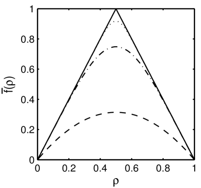
The networks we consider are Poisson random networks from $\mathcal{G}(N,k_{\rm avg}/N)$. The thresholds $\phi_{{\rm on}}$ and $\phi_{{\rm off}}$ are distributed uniformly on $[0,1/2)$ and $[1/2,1)$, respectively. This distribution results in the probabilistic response function (see Figure 2)

$$\bar{f}(\phi)=\left\{\begin{array}[]{lrl}2\phi\hfill&\mathrm{if}&0\leq\phi<1/2,\\ 2-2\phi\hfill&\mathrm{if}&1/2\leq\phi\leq 1.\end{array}\right.$$ (17)

The tent map is a well-known chaotic map of the unit interval (Alligood et al., 1996). We thus expected that the limited imitation model with this probabilistic response function to exhibit similarly interesting behavior.

Figure 2: The tent map probabilistic response function $\bar{f}(\rho)$, Eqn. (17), used in the limited imitation contagion model. This is compared to the edge maps $g(\rho;k_{\rm avg})=g(\rho;p_{k},\bar{f})$, Eqn. (10), with $k_{\rm avg}=1,10,100$ (dashed, dot-dashed, and dotted lines). These $p_{k}$ are Poisson distributions with mean $k_{\rm avg}$. As $k_{\rm avg}$ increases, $g(\rho;k_{\rm avg})$ increases to $\bar{f}(\rho)$.

V.1 Analysis of the dense limit

When the network is in the dense limit (Section III.2), the dynamics follow $\phi(t+1)=\Phi(\phi(t);\alpha)$, where

$$\Phi(\phi;\alpha) =\alpha\bar{f}(\phi)+(1-\alpha)\phi$$ (18)

$$=\left\{\begin{array}[]{lrl}(1+\alpha)\phi&\mathrm{if}&0\leq\phi<1/2,\\ (1-3\alpha)\phi+2\alpha&\mathrm{if}&1/2\leq\phi\leq 1.\end{array}\right.$$

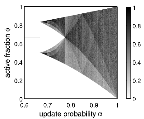
Solving for the fixed points of $\Phi(\phi;\alpha)$, we find one at $\phi=0$ and another at $\phi=2/3$. When $\alpha<2/3$, the nonzero fixed point is attracting for all initial conditions except $\phi=0$. When $\alpha=2/3$, $[1/2,5/6]$ is an interval of period-2 centers. Any orbit will eventually land on one of these period-2 orbits. When $\alpha>2/3$, this interval of period-2 centers ceases to exist, and more complicated behavior ensues. Figure 3 shows the bifurcation diagram for $\Phi(\phi;\alpha)$. From the bifurcation diagram, the orbit appears to cover dense subsets of the unit interval when $\alpha>2/3$. The bifurcation diagram appears like that of the tent map (not shown; see Alligood et al. (1996); Dodds et al. (2013)) except the branches to the right of the first bifurcation point are separated here by the interval of period-2 centers.

Figure 3: Bifurcation diagram for the dense map $\Phi(\phi;\alpha)$, Eqn. (18). This was generated by iterating the map at 1000 $\alpha$ values between 0 and 1. The iteration was carried out with 3 random initial conditions for 10000 time steps each, discarding the first 1000. The $\phi$-axis contains 1000 bins and the invariant density, shown by the grayscale value, is normalized by the maximum for each $\alpha$. With $\alpha<2/3$, all trajectories go to the fixed point at $\phi=2/3$.

The effect of conformists, an aside

Suppose some fraction $c$ of the population is made up of individuals without any off-threshold (alternatively, each of their off-thresholds $\phi_{{\rm off}}=1$). These individuals are conformist or purely pro-social in the sense that they are content with being part of the majority. For simplicity, assume $\alpha=1$. The map $\Phi(\phi;c)=2\phi$ for $0\leq\phi<1/2$ and $2-2(1-c)\phi$ for $1/2\leq\phi\leq 1$. If $c>1/2$, then the equilibrium at 2/3 is stable. Pure conformists, then, have a stabilizing effect on the process. We expect a similar effect when the network is not dense.

V.2 Mean-field

Here we mention the methods which were used to compute the mean-field maps derived in Section IV. In this specific example, we can write the degree-dependent map $F_{k}(\rho;\bar{f})$ in terms of incomplete regularized beta functions $I_{z}(a,b)$ (NIST, 2012). Since $\bar{f}$ is understood to be the tent map, we will write $F_{k}(\rho;\bar{f})=F_{k}(\rho)$. We find that

$$F_{k}(\rho)=2\rho-4\rho I_{\rho}(M,k-M),$$ (19)

where we have let $M=\lfloor k/2\rfloor$ for clarity ($\lfloor\cdot\rfloor$ and $\lceil\cdot\rceil$ are the floor and ceiling functions). The details of this derivation are given in Appendix B.

The map $g(\rho;p_{k},\bar{f})$ is parameterized here by the network parameter $k_{\rm avg}$, since $p_{k}$ is fixed as a Poisson distribution with mean $k_{\rm avg}$ and $\bar{f}$ is the tent map, and we write it as simply $g(\rho;k_{\rm avg})$. To evaluate $g(\rho;k_{\rm avg})$, we compute $F_{k}(\rho)$ using Eqn. (19) and constrain the sum in Eqn. (10) to values of $k$ with $\lfloor k_{\rm avg}-3\sqrt{k_{\rm avg}}\rfloor\leq k\leq\lceil k_{\rm avg}+3\sqrt{k_{\rm avg}}\rceil$. This computes contributions to within three standard deviations of the average degree in the network, requiring only $O(\sqrt{k_{\rm avg}})$ evaluations of Eqn. (19). The representation in Eqn. (19) allows for quick numerical evaluation of $F_{k}(\rho)$ for any $k$, which we performed in MATLAB.

In Figure 2, we show $g(\rho;k_{\rm avg})$ for $k_{\rm avg}=1,10,$ and 100. We confirm the conclusions of Section IV.2: $g(\rho;k_{\rm avg})$ is bounded above by $\bar{f}(\rho)$, and $g(\rho;k_{\rm avg})\nearrow\bar{f}(\rho)$ as $k_{\rm avg}\to\infty$. Convergence is slowest at $\rho=1/2$, where the kink exhibited by the tent map has been smoothed out by the effect of the Bernstein operator.

V.3 Simulations

We performed stochastic simulations of the limited imitation model for the D-F, P-F, and P-R designs, in the abbreviations of Table 1. See Supplemental Material at [URL will be inserted by publisher] for the Python code. Unless otherwise noted, $N=10^{4}$. For all of the bifurcation diagrams, the first 3000 time steps were considered transient and discarded, and the invariant density of $\rho$ was calculated from the following 1000 points. For plotting purposes, the invariant density was normalized by its maximum at those parameters. For example, in Figure 3 we plot $P(\phi|\alpha)/\max_{\phi}P(\phi|\alpha)$ rather than the raw density $P(\phi|\alpha)$.

To compare the mean-field theory to those simulations, we numerically iterated the edge map $\rho(t+1)=G\left(\rho(t);k_{\rm avg},\alpha\right)$ for different values of $\alpha$ and $k_{\rm avg}$. We then created bifurcation diagrams of the possible behavior in the mean-field as was done for the simulations.

V.4 Results

Figure 4: Deterministic (D-F) dynamics on a small network. Here, $N=100$ and $k_{\rm avg}=17$. The upper plot shows individual node states as a raster plot (black = active), sorted by their eventual level of activity. The lower plot shows the total number of active nodes over time. We see that the contagion takes off, followed by a transient period of unstable behavior until time step 80, when the system enters a macroperiod-4 orbit. Note that individual nodes exhibit different microperiods (explained in Sec. V.4).

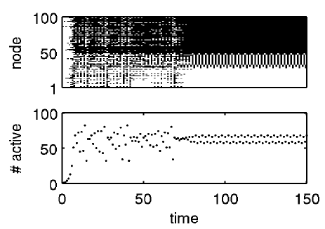
To provide a feel for the deterministic dynamics, we show the result of running the D-F model on a small network in Figure 4. Here, $N=100$ and $k_{\rm avg}=17$. Starting from a single initially active node at $t=0$, the active population grows monotonically over the next 6 time steps. From $t=6$ to $t=80$, the transient time, the active fraction varies in a similar manner to the dynamics in the stochastic and mean-field cases. After the transient, the state collapses into a period-4 orbit. We call the overall period of the system its “macroperiod,” while individual nodes may exhibit different “microperiods.” Note that the macroperiod is the lowest common multiple of the individual nodes’ microperiods. In Figure 4, we observe microperiods 1, 2, and 4 in the timeseries of individual node activity. In other networks, we have observed up to macroperiod 240 (Dodds et al., 2013). A majority of the nodes end up frozen in the on or off state, with approximately $20\%$ of the nodes exhibiting cyclical behavior after collapse. The focus of this paper has been the analysis of the on-off threshold model, and the D-F case has not been as amenable to analysis as the stochastic cases. We offer a deeper examination through simulation of the deterministic case in Dodds et al. (2013).

Figure 5: The 3-dimensional bifurcation diagram computed from the mean-field theory. The axes X = average degree $k_{\rm avg}$, Y = update probability $\alpha$, and Z = active edge fraction $\rho$. The discontinuities of the surface are due to the limited resolution of our simulations. See Figure 6 for the parameters used. This was visualized using Paraview. See Supplemental Material at [URL will be inserted by publisher] for the underlying data.

Figure 6: Mean-field theory bifurcation diagram slices for various fixed values of $k_{\rm avg}$ and $\alpha$. The top row (a–c) shows slices for fixed $k_{\rm avg}$. As $k_{\rm avg}\to\infty$, the $k_{\rm avg}$-slice bifurcation diagram asymptotically approaches the bifurcation diagram for the dense map, Figure 3. Note that the location of the first period-doubling bifurcation point approaches 2/3, and the bifurcation diagram more closely resembles Fig. 3, as $k_{\rm avg}\to\infty$. The bottom row (d–f) shows slices for fixed $\alpha$. The resolution of the simulations was $\alpha=0.664,0.665,\ldots,1$, $k_{\rm avg}=1,1.33,\ldots,100$, and $\rho$ bins were made for 1000 points between 0 and 1.

Figure 7: Bifurcation diagram from fully stochastic (P-R) simulations, made in the same way as Figure 6. The bifurcation structure of these stochastic simulations matches that of the mean-field theory (Figure 6), albeit with some blurring.

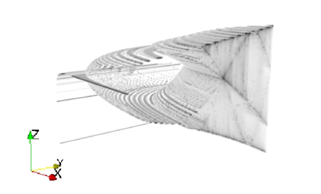
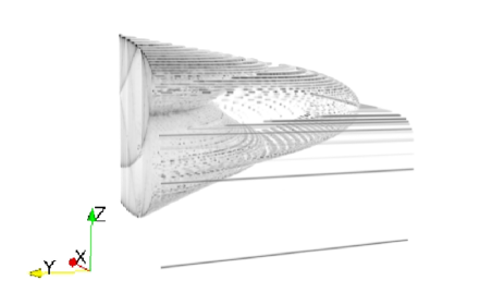
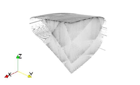
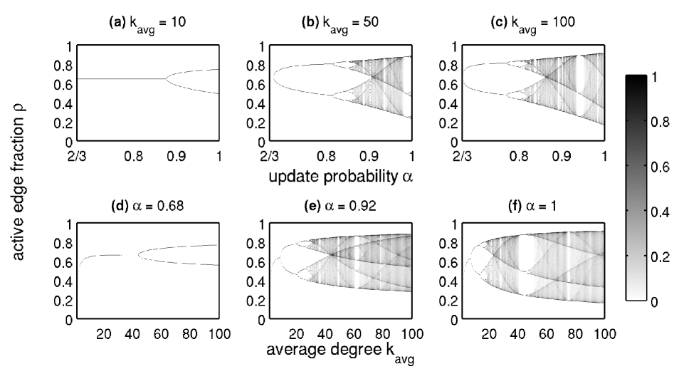
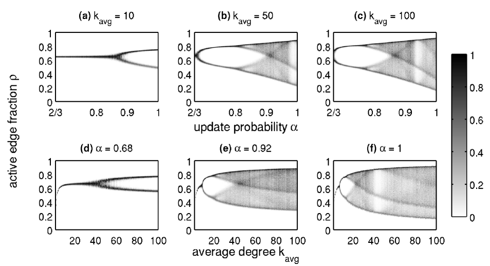
We explore the mean-field dynamics by examining the limiting behavior of the active edge fraction $\rho$ under the map $G\left(\rho;k_{\rm avg},\alpha\right)$. We simulated the map dynamics for a mesh of points in the $(k_{\rm avg},\alpha)$ plane. We plot the 3-dimensional (3-d) bifurcation structure of the mean-field theory in Figure 5. We also show 2-d bifurcation plots for fixed $k_{\rm avg}$ and $\alpha$ slices through this volume in Figures 6 and 7. For more visualizations of this bifurcation structure, including movies of the bifurcation diagram as the parameters are dialed and individual node dynamics, see Supplemental Material at [URL will be inserted by publisher]. In all cases, the invariant density of $\rho$ is normalized by its maximum for that $(k_{\rm avg},\alpha)$ pair and indicated by the grayscale value.

The mean-field map dynamics exhibit period-doubling bifurcations in both parameters $k_{\rm avg}$ and $\alpha$. Visualizing the bifurcation structure in 3-d (Figure 5) shows interlacing period-doubling cascades in the two parameter dimensions. These bifurcations are more clearly resolved when we take slices of the volume for fixed parameter values. The mean-field theory (Figure 6) closely matches the P-R simulations (Figure 7). The first derivative $\frac{\partial G}{\partial\rho}(\rho;k_{\rm avg},\alpha)<\frac{\partial\Phi}{\partial\rho}(\rho;\alpha)$ for any finite $k_{\rm avg}$, so the bifurcation point $\alpha=2/3$ which we found for the dense map $\Phi$ is an upper bound for the first bifurcation point of $G$. The actual location of the first bifurcation point depends on $k_{\rm avg}$, but $\alpha=2/3$ becomes more accurate for higher $k_{\rm avg}$ (it is an excellent approximation in Figures 6c and 7c, where $k_{\rm avg}=100$). When $\alpha=1$, the first bifurcation point occurs at $k_{\rm avg}\approx 7$.

The bifurcation diagram slices resemble each other and evidently fall into the same universality class as the logistic map (Feigenbaum, 1978, 1979). This class contains all 1-d maps with a single, locally-quadratic maximum. Due to the properties of the Bernstein polynomials, $F_{k}(\rho;\bar{f})$ will universally have such a quadratic maximum for any concave down, continuous $\bar{f}$ (Phillips, 2003). So this will also be true for $g(\rho;k_{\rm avg},\bar{f})$ with $k_{\rm avg}$ finite, and we see that $k_{\rm avg}$ partially determines the amplitude of that maximum in Figure 2. Thus $k_{\rm avg}$ acts as a bifurcation parameter. The parameter $\alpha$ tunes between $G\left(\rho;k_{\rm avg},1\right)=g(\rho;k_{\rm avg},\bar{f})$ and $G\left(\rho;k_{\rm avg},0\right)=\rho$, so it has a similar effect. Note that the tent map $\bar{f}$ and the dense limit map $\Phi$ are kinked at their maxima, so their bifurcation diagrams are qualitatively different from those of the mean-field. The network, by locally averaging the node interactions, causes the mean-field behavior to fall into a different universality class than the individual response function map.

VI Conclusions

We have described a very general class of synchronous or asynchronous, binary state dynamics occurring on networks. We obtained an exact master equation and showed that, when random networks are sufficiently dense, the networked dynamics approach those of the fully-connected case. We developed a mean-field theory and found that it also predicted the same limiting behavior. The convergence of the mean-field map to the average response function is related to the Bernstein polynomials, allowing us to employ many previous results in order to analyze the mean-field map equation. We also extended those mean-field equations to correlated random networks. We expect that a rigorous mathematical justification can be given for the mean-field theory of the general influence model on annealed graphs using a condensation theorem for configuration model networks.

The general model we describe was motivated by the limited imitation model of social contagion. We see that including an aversion to total conformity results in more complicated, even chaotic dynamics, as opposed to the simple spreading behavior typically seen in the single threshold case. The theory developed for the general case successfully captured the behavior of the stochastic network dynamics. We have focused on the rich structure of bifurcations as the two parameters, update synchronicity $\alpha$ and average degree $k_{\rm avg}$, were varied. We see that the universality class of the dynamics matches those of the logistic map. Using the mean-field theory, we can understand this as a result of the smoothing effect of the Bernstein polynomials on the tent map average response function. However, this universality class will appear for any unimodular, concave down stochastic response function.

The deterministic case, which we have barely touched on, merits further study (see Dodds et al., 2013). In particular, we would like to characterize the distribution of periodic sinks, how the collapse time scales with system size, and how similar the transient dynamics are to the mean-field dynamics.

Furthermore, the model should be tested on realistic networks. These could include power law or small world random networks, or real social networks gleaned from data. One possibility would be to compare data such as food choices (Pachucki et al., 2011) or Facebook likes (Ugander et al., 2012) to the model behavior. In a manner similar to Melnik et al. (2011), one could evaluate the accuracy of the mean-field theory for real networks.

Finally, the ultimate usefulness of these social models relies on a better understanding of social dynamics themselves. Characterization of people’s “real” response functions is therefore critical (some work has gone in this direction; see Centola, 2010, 2011; Romero et al., 2011; Ugander et al., 2012). Comparison of model output to large data sets, such as observational data from social media or online experiments, is an area for further experimentation. This might lead to more complicated context- and history-dependent models. As we collect more data and refine experiments, the eventual goal of quantifiably predicting social behavior, including fashions and trends, seems achievable.

Appendix A Proof of Lemma 1

Lemma 1.

For $k\geq 1$, let $f_{k}$ be continuous real-valued functions on a compact domain $X$ with $f_{k}\to f$ uniformly. Let $p_{k}$ be a probability mass function on $\mathbb{Z}^{+}$ parameterized by its mean $\mu$ and with standard deviation $\sigma(\mu)$, assumed to be $o(\mu)$. Then,

$$\lim_{\mu\to\infty}\left(\sum_{k=0}^{\infty}p_{k}f_{k}\right)=f.$$

Proof.

Suppose $0\leq a<1$ and let $K=\lfloor\mu-\mu^{a}\rfloor$. Then,

$$g=\sum_{k=0}^{\infty}p_{k}f_{k}=\sum_{k=0}^{K}p_{k}f_{k}+\sum_{k=K+1}^{\infty}p_{k}f_{k}.$$ (20)

Since $f_{k}\to f$ uniformly as $k\to\infty$, for any $\epsilon>0$ we can choose $\mu$ large enough that

$$|f_{k}(x)-f(x)|<\epsilon$$ (21)

for all $k>K$ and all $x\in X$. Without loss of generality, assume that $|f_{k}|\leq 1$ for all $k$. Then,

$$|g-f|\leq\left(\frac{\sigma}{\mu^{a}}\right)^{2}+\epsilon.$$

The $\sigma/\mu^{a}$ term is a consequence of the Chebyshev inequality (Bollobás, 2001) applied to the first sum in (20). Since $\sigma$ grows sublinearly in $\mu$, this term vanishes for some $0\leq a<1$ when we take the limit $\mu\to\infty$. The $\epsilon$ term comes from using (21) in the second sum in (20), and it can be made arbitrarily small. ∎

Appendix B Beta function representation of $F_{k}$

We now show how, when $\bar{f}$ is the tent map (17), the map $F_{k}(\rho;\bar{f})$ can be written in terms of incomplete regularized beta functions. First, use the piecewise form of Eqn. (17) to write

$$F_{k}(\rho) =\sum_{j=0}^{M}\binom{k}{j}\rho^{j}(1-\rho)^{k-j}\left(\frac{2j}{k}\right)$$

$$\quad+\sum_{j=M+1}^{k}\binom{k}{j}\rho^{j}(1-\rho)^{k-j}\left(2-\frac{2j}{k}\right)$$

$$=2-2\rho-2\sum_{j=0}^{M}\binom{k}{j}\rho^{j}(1-\rho)^{k-j}$$

$$\quad+\left(\frac{4}{k}\right)\sum_{j=0}^{M}\binom{k}{j}\rho^{j}(1-\rho)^{k-j}j.$$ (22)

We have used the fact that the binomial distribution $\binom{k}{j}\rho^{j}(1-\rho)^{k-j}$ sums to one and has mean $k\rho$. For $n\leq M$, we have the identity

$$\sum_{j=0}^{M}(j)_{n}\binom{k}{j}\rho^{j}(1-\rho)^{k-j}=\rho^{n}(k)_{n}I_{1-\rho}(k-M,M-n+1)$$ (23)

where $I_{x}(a,b)$ is the regularized incomplete beta function and $(k)_{n}=k(k-1)\cdots(k-(n-1))$ is the falling factorial (Winkler et al., 1972; NIST, 2012). This is an expression for the partial (up to $M$) $n$th factorial moment of the binomial distribution with parameters $k$ and $\rho$. Note that when $n=0$ we recover the well-known expression for the binomial cumulative distribution function. From Eqns. (22) and (23), we arrive at Eqn. (19).

References

- Coombes et al. (2006) S. Coombes, B. Doiron, K. Josić, and E. Shea-Brown, Philosophical Transactions of the Royal Society A: Mathematical, Physical and Engineering Sciences 364, 3301 (2006).
- Milo et al. (2002) R. Milo, S. Shen-Orr, S. Itzkovitz, N. Kashtan, D. Chklovskii, and U. Alon, Science 298, 824 (2002).
- Bascompte (2009) J. Bascompte, Science 325, 416 (2009).
- Rohani et al. (2010) P. Rohani, X. Zhong, and A. King, Science 330, 982 (2010).
- Ugander et al. (2012) J. Ugander, L. Backstrom, C. Marlow, and J. Kleinberg, PNAS 109, 5962 (2012).
- Centola (2010) D. Centola, Science 329, 1194 (2010).
- Aldana et al. (2003) M. Aldana, S. Coppersmith, and L. P. Kadanoff, in Perspectives and Problems in Nonlinear Science, edited by E. Kaplan, J. E. Marsden, and K. R. Sreenivasan (Springer, New York, 2003), chap. 2, pp. 23–90, http://arxiv.org/abs/nlin/0204062.
- Stauffer and Aharony (1994) D. Stauffer and A. Aharony, Introduction to Percolation Theory (Taylor and Francis, London, 1994), 2nd ed.
- Newman (2003) M. E. J. Newman, SIAM Review 45, 167 (2003).
- Schneidman et al. (2006) E. Schneidman, M. J. Berry, R. Segev, and W. Bialek, Nature 440, 1007 (2006).
- Campbell et al. (2011) C. Campbell, S. Yang, R. Albert, and K. Shea, Proceedings of the National Academy of Sciences 108, 197 (2011).
- Granovetter (1978) M. Granovetter, American Journal of Sociology 83, 1420 (1978).
- Granovetter and Soong (1986) M. Granovetter and R. Soong, Journal of Economic Behavior and Organization 7, 83 (1986).
- Galam (2008) S. Galam, International Journal of Modern Physics C 19, 409 (2008).
- Schelling (1971) T. C. Schelling, Journal of Mathematical Sociology 1, 143 (1971).
- Schelling (1973) T. C. Schelling, Journal of Conflict Resolution 17, 381 (1973).
- Watts (2002) D. J. Watts, PNAS 99, 5766 (2002).
- Dodds and Watts (2004) P. S. Dodds and D. J. Watts, Phys. Rev. Lett. 92, 218701 (2004).
- Dodds et al. (2013) P. S. Dodds, K. D. Harris, and C. M. Danforth, Phys. Rev. Lett. 110, 158701 (2013), http://arxiv.org/abs/1208.0255.
- Simmel (1957) G. Simmel, American Journal of Sociology 62, 541 (1957).
- Bollobás (2001) B. Bollobás, Random Graphs (Cambridge University Press, 2001), 2nd ed.
- Note (1) Note1, when there are isolated nodes, their degrees are 0, and thus the denominator in the master equation is zero and is singular. If the initial network contains isolated nodes, we set all entries in the corresponding rows of to zero.
- Gleeson (2008) J. P. Gleeson, Phys. Rev. E 77, 046117 (2008).
- West (2001) D. B. West, Introduction to Graph Theory (Prentice Hall, Upper Saddle River, NJ, 2001), 2nd ed.
- Oliveira (2010) R. I. Oliveira (2010), http://arxiv.org/abs/0911.0600, eprint 0911.0600.
- Derrida and Pomeau (1986) B. Derrida and Y. Pomeau, Europhys. Lett. 1, 45 (1986).
- Melnik et al. (2011) S. Melnik, A. Hackett, M. A. Porter, P. J. Mucha, and J. P. Gleeson, Phys. Rev. E 83, 036112 (2011).
- Phillips (2003) G. M. Phillips, Interpolation and Approximation by Polynomials (Springer, 2003), see chapter 7.
- Peña (1999) J. M. Peña, ed., Shape Preserving Representations in Computer-Aided Geometric Design (Nova Science Publishers, Inc, 1999).
- Payne et al. (2011) J. L. Payne, K. D. Harris, and P. S. Dodds, Phys. Rev. E 84, 016110 (2011), URL http://link.aps.org/doi/10.1103/PhysRevE.84.016110.
- Dodds et al. (2011) P. S. Dodds, K. D. Harris, and J. L. Payne, Phys. Rev. E 83, 056122 (2011), URL http://link.aps.org/doi/10.1103/PhysRevE.83.056122.
- Gleeson and Cahalane (2007) J. P. Gleeson and D. J. Cahalane, Phys. Rev. E 75, 056103 (2007), URL http://link.aps.org/doi/10.1103/PhysRevE.75.056103.
- Alligood et al. (1996) K. T. Alligood, T. D. Sauer, and J. A. Yorke, Chaos: An Introduction to Dynamical Systems (Springer, 1996).
- NIST (2012) NIST, Digital Library of Mathematical Functions (2012), http://dlmf.nist.gov.
- Feigenbaum (1978) M. J. Feigenbaum, Journal of Statistical Physics 19, 25 (1978).
- Feigenbaum (1979) M. J. Feigenbaum, Journal of Statistical Physics 21, 669 (1979).
- Pachucki et al. (2011) M. A. Pachucki, P. F. Jacques, and N. A. Christakis, American Journal of Public Health 101, 2170 (2011).
- Centola (2011) D. Centola, Science 334, 1269 (2011).
- Romero et al. (2011) D. M. Romero, B. Meeder, and J. Kleinberg, in Proc. 20th ACM International World Wide Web Conference (2011).
- Winkler et al. (1972) R. L. Winkler, G. M. Roodman, and R. R. Britney, Management Science 19, 290 (1972).