GPU accelerated maximum cardinality matching algorithms for bipartite graphs

Abstract

We design, implement, and evaluate GPU-based algorithms for the maximum cardinality matching problem in bipartite graphs. Such algorithms have a variety of applications in computer science, scientific computing, bioinformatics, and other areas. To the best of our knowledge, ours is the first study which focuses on GPU implementation of the maximum cardinality matching algorithms. We compare the proposed algorithms with serial and multicore implementations from the literature on a large set of real-life problems where in majority of the cases one of our GPU-accelerated algorithms is demonstrated to be faster than both the sequential and multicore implementations.

1 Introduction

Bipartite graph matching is one of the fundamental problems in graph theory and combinatorial optimization. The problem asks for a maximum set of vertex disjoint edges in a given bipartite graph. It has many applications in a variety of fields such as image processing [17], chemical structure analysis [15], and bioinformatics [2] (see also another two discussed by Burkard et al. [4, Section 3.8]). Our motivating application lies in solving sparse linear systems of equations, as algorithms for computing a maximum cardinality bipartite matching are run routinely in the related solvers. In this setting, bipartite matching algorithms are used to see if the associated coefficient matrix is reducible; if so, substantial savings in computational requirements can be achieved [7, Chapter 6].

Achieving good parallel performance on graph algorithms is challenging, because they are memory bounded, and there are poor localities of the memory accesses. Moreover, because of the irregularity of the computations, it is difficult to exploit concurrency. Algorithms for the matching problem are no exception. There have been recent studies that aim to improve the performance of matching algorithms on multicore and manycore architectures. For example, Vasconcelos and Rosenhahn [18] propose a GPU implementation of an algorithm for the maximum weighted matching problem on bipartite graphs. Fagginger Auer and Bisseling [10] study an implementation of a greedy graph matching on GPU. Çatalyürek et al. [5] propose different greedy graph matching algorithms for multicore architectures. Azad et al. [1] introduce several multicore implementations of maximum cardinality matching algorithms on bipartite graphs.

We propose GPU implementations of two maximum cardinality matching algorithms. We analyze their performance and employ further improvements. We thoroughly evaluate their performance with a rigorous set of experiments on many bipartite graphs from different applications. The experimental results conclude that one of the proposed GPU-based implementation is faster than its existing multicore counterparts.

The rest of this paper is organized as follows. The background material, some related work, and a summary of contributions are presented in Section 2. Section 3 describes the proposed GPU algorithms. The comparison of the proposed GPU-based implementations with the existing sequential and multicore implementations is given in Section 4. Section 5 concludes the paper.

2 Background and contributions

A bipartite graph $G=(V_{1}\cup V_{2},E)$ consists of a set of vertices $V_{1}\cup V_{2}$ where $V_{1}\cap V_{2}=\emptyset$, and a set of edges $E$ such that for each edge, one of the endpoints is in $V_{1}$ and other is in $V_{2}$. Since our motivation lies in the sparse matrix domain, we will refer to the vertices in the two classes as row and column vertices.

A matching ${\cal M}$ in a graph $G$ is a subset of edges $E$ where a vertex in $V_{1}\cup V_{2}$ is in at most one edge in ${\cal M}$. Given a matching ${\cal M}$, a vertex $v$ is said to be matched by ${\cal M}$ if $v$ is in an edge of ${\cal M}$, otherwise $v$ is called unmatched. The cardinality of a matching ${\cal M}$, denoted by $|{\cal M}|$, is the number of edges in ${\cal M}$. A matching ${\cal M}$ is called maximum, if no other matching ${\cal M}^{\prime}$ with $|{\cal M}^{\prime}|>|{\cal M}|$ exists. For a matching ${\cal M}$, a path ${\cal P}$ in $G$ is called an ${\cal M}$-alternating if its edges are alternately in ${\cal M}$ and not in ${\cal M}$. An ${\cal M}$-alternating path ${\cal P}$ is called $M$-augmenting if the start and end vertices of ${\cal P}$ are both unmatched.

There are three main classes of algorithms for finding the maximum cardinality matchings in bipartite graphs. The first class of algorithms is based on augmenting paths (see a detailed summary by Duff et al. [8]). Push-relabel-based algorithms form a second class [12]. A third class, pseudoflow algorithms, is based on a more recent work [13]. There are $\mathcal{O}(\sqrt{n}\tau)$ algorithms in the first two classes (e.g., Hopcroft-Karp algorithm [14] and a variant of the push relabel algorithm [11]), where $n$ is the number of vertices and $\tau$ is the number of edges in the given bipartite graph. This is asymptotically best bound for practical algorithms. Most of the other known algorithms in the first two classes and in the third class have the running time complexity of $\mathcal{O}(n\tau)$. These three classes of algorithms are described and compared in a recent study [16]. It has been demonstrated experimentally that the champions of the first two families are comparable in performance and better than that of the third family. Since we investigate GPU acceleration of augmenting-path-based algorithms, a brief description of them is given below (the reader is invited to two recent papers [8, 16] and the original resources cited in those papers for other algorithms).

Algorithms based on augmenting paths follow the following common pattern. Given an initial matching ${\cal M}$ (possible empty), they search for an ${\cal M}$-augmenting path ${\cal P}$. If none exists, then the matching ${\cal M}$ is maximum by a theorem of Berge [3]. Otherwise, the augmenting path ${\cal P}$ is used to increase the cardinality of ${\cal M}$ by setting ${\cal M}={\cal M}\oplus E({\cal P})$ where $E({\cal P})$ is the edge set of the path ${\cal P}$, and ${\cal M}\oplus E({\cal P})=({\cal M}\cup E({\cal P}))\setminus({\cal M}\cap E({\cal P}))$ is the symmetric difference. This inverts the membership in ${\cal M}$ for all edges of ${\cal P}$. Since both the first and the last edge of ${\cal P}$ were unmatched in ${\cal M}$, we have $|{\cal M}\oplus E({\cal P})|=|{\cal M}|+1$. The augmenting-path-based algorithms differ in the way these augmenting paths are found and the associated augmentations are realized. They mainly use either breadth-first-search (BFS), or depth-first-search (DFS), or combination of these two techniques to locate and perform the augmenting paths.

Multicore counterparts of a number of augmenting-path based algorithms are proposed in a recent work [1]. The parallelization of these algorithms is achieved by using atomic operations at BFS and/or DFS steps of the algorithm. Although using atomic operations might not harm the performance on a multicore machine, they should be avoided in a GPU implementation because of very large number of concurrent thread executions.

As a reasonably efficient DFS is not feasible with GPUs, we accelerate two BFS-based algorithms, called HK [14] and HKDW [9]. HK has the best known worst-case running time complexity of $O(\sqrt{n}\tau)$ for a bipartite graph with $n$ vertices and $\tau$ edges. HKDW is a variant of HK and incorporates techniques to improve the practical running time while having the same worst-case time complexity. Both of these algorithms use BFS to locate the shortest augmenting paths from unmatched columns, and then use DFS-based searches restricted to a certain part of the input graph to augment along a maximal set of disjoint augmenting paths. HKDW performs another set of DFS-based searches to augment using the remaining unmatched rows. As is clear, the DFS-based searches will be a big obstacle to achieve efficiency. In order to overcome this hurdle, we propose a scheme which alternates the edges of a number of augmenting paths with a parallel scheme that resembles to a breadth expansion in BFS. The proposed scheme offers a high degree of parallelism but does not guarantee a maximal set of augmentations, potentially increasing the worst case time complexity to $O(n\tau)$ on a sequential machine. In other words, we trade theoretical worst case time complexity with a higher degree of parallelism to achieve better practical running time with a GPU.

3 Methods

We propose two algorithms for the GPU implementation of maximum cardinality matching. These algorithms use BFS to find augmenting paths, speculatively perform some of them, and fix any inconsistencies that can be resulting from speculative augmentations.

The overall structure of the first GPU-based algorithm is given in Algorithm 1, APsB. It largely follows the common structure of most of the existing sequential algorithms, and corresponds to HK. It performs a combined BFS starting from all unmatched columns to find unmatched rows, thus locating augmenting paths. Some of those augmentations are then realized using a function called Alternate (will be described later). The parallelism is exploited inside the InitBfsArray, BFS, Alternate, and FixMatching functions. Algorithm 1 is given the adjacency list of the bipartite graph with its number of rows and columns. Any prior matching is given in $rmatch$ and $cmatch$ arrays as follows: $rmatch[r]=c$ and $cmatch[c]=r$, if the row $r$ is matched to the column $c$; $rmatch[r]=-1$, if $r$ is unmatched; $cmatch[c]=-1$, if $c$ is unmatched.

Data: $cxadj,cadj,nc,nr,rmatch,cmatch$

1

2$augmenting\_path\_found\leftarrow{\bf true}$;

3 while $augmenting\_path\_found$ do

4       $bfs\_level\leftarrow{\sc L_{0}}{}$;

5       InitBfsArray$(bfs\_array,cmatch,{\sc L_{0}}{})$;

6       $vertex\_inserted\leftarrow{\bf true}$;

7       while $vertex\_inserted$ do

8             $predecessor\leftarrow$Bfs$(bfs\_level,bfs\_array,cxadj,cadj,nc,rmatch,$

9                                         $vertex\_inserted,augmenting\_path\_found)$;

10             if $augmenting\_path\_found$ then

11                   $break$;

12            

13            $bfs\_level\leftarrow bfs\_level+1$;

14      

15      $\langle cmatch,rmatch\rangle\leftarrow$ Alternate $(cmatch,rmatch,nc,predecessor)$;

16       $\langle cmatch,rmatch\rangle\leftarrow$ FixMatching $(cmatch,rmatch)$;

17      

Algorithm 1 Shortest augmenting paths (APsB)

The outer loop of Algorithm 1 iterates until no more augmenting paths are found, thereby guaranteeing a maximum matching. The inner loop is responsible from completing the breadth-first-search of the augmenting paths. A single iteration of this loop corresponds to a level of BFS. The inner loop iterates until all shortest augmenting paths are found. Then, the edges in these shortest augmenting paths are alternated inside Alternate function. Unlike the sequential HK algorithm, APsB does not find a maximal set of augmenting paths.

By removing the lines 9 and 10 of Algorithm 1, another matching algorithm is obtained. This method will continue with the BFSs until all possible unmatched rows are found; it can be therefore considered as the GPU implementation of the HKDW algorithm. This variant is called APFB.

Data: $bfs\_level,bfs\_array,cxadj,cadj,nc,rmatch,$

             $vertex\_inserted,augmenting\_path\_found$

1

2$process\_cnt\leftarrow{\sc getProcessCount}(nc)$;

3 for $i$ from $0$ to $process\_cnt-1$ do

4       $col\_vertex\leftarrow i\times tot\_thread\_num+tid$;

5       if $bfs\_array[col\_vertex]$ $=$ $bfs\_level$ then

6             for $j$ from $cxadj[col\_vertex]$ to $cxadj[col\_vertex+1]$  do

7                   $neighbor\_row\leftarrow cadj[j]$;

8                   $col\_match\leftarrow rmatch[neighbor\_row]$;

9                   if $col\_match>-1$ then

10                         if $bfs\_array[col\_match]$ $=$ ${\sc L_{0}}{}$ $-1$  then

11                               $vertex\_inserted\leftarrow{\bf true}$;

12                               $bfs\_array[col\_match]\leftarrow bfs\_level+1$;

13                               $predeccesor[neighbor\_row]\leftarrow col\_vertex$;

14                              

15                        

16                  else

17                         if $col\_match$=$-1$ then

18                               $rmatch[neighbor\_row]\leftarrow-2$;

19                               $predeccesor[neighbor\_row]\leftarrow col\_vertex$;

20                               $augmenting\_path\_found\leftarrow{\bf true}$;

21                              

22                        

23                  

24            

25      

26

Algorithm 2 BFS Kernel Function-1 (GPUBFS)

We propose two implementations of the BFS kernel. Algorithm 2 is the first one. The BFS kernel is responsible from a single level BFS expansion. That is, it takes the set of vertices at a BFS level and adds the union of the unvisited neighbors of those vertices as the next level of vertices. Initially, the input $bfs\_array$ filled with $bfs\_array[c]={\sc L_{0}}{}-1$ if $cmatch[c]>-1$ and $bfs\_array[c]={\sc L_{0}}{}$ if $cmatch[c]=-1$ by a simple InitBfsArray kernel (${\sc L_{0}}{}$ denotes BFS start level).

The GPU threads partition the columns vertices in a single dimension. Each thread with id $tid$ is assigned a number of columns which is obtained via the following function:

$getProcessCount(nc)=\left\{\begin{array}[]{l l}\lceil\frac{nc}{tot\_thread\_num}\rceil&\text{if $tid<nc\bmod tot\_thread\_num$,}\\ \lfloor\frac{nc}{tot\_thread\_num}\rfloor&\text{otherwise.}\end{array}\right.$

Once the number of columns are obtained, the threads traverse their first assigned column vertex. The indices of the columns assigned to a thread differ by $tot\_thread\_num$ to allow coalesced global memory accesses. Threads traverse the neighboring row vertices of the current column, if its BFS level is equal to the current $bfs\_level$. If a thread encounters a matched row during the traversal, its matching column is retrieved. If the column is not traversed yet, its $bfs\_level$ is marked on $bfs\_array$. On the other hand, when a thread encounters an unmatched row, an augmenting path is found. In this case, the match of the neighbor row is set to $-2$, and this information is used by Alternate later.

Data: $cmatch,rmatch,nc,nr,predecessor$

1

2$process\_vcnt\leftarrow{\sc getProcessCount}(nr)$;

3 for $i$ from $0$ to $process\_vcnt-1$ do

4       $row\_vertex\leftarrow i\times tot\_thread\_num+tid$;

5       if $rmatch[row\_vertex]$ $=$ $-2$ then

6             while $row\_vertex\neq-1$ do

7                   $matched\_col\leftarrow predecessor[row\_vertex]$;

8                   $matched\_row\leftarrow cmatch[matched\_col]$ ;

9                   if predecessor[matched_row] $=$ matched_col then

10                         $break$;

11                        

12                  $cmatch[matched\_col]\leftarrow row\_vertex$;

13                   $rmatch[row\_vertex]\leftarrow matched\_col$;

14                   $row\_vertex\leftarrow matched\_row$;

15                  

16            

17      

Algorithm 3 Alternate

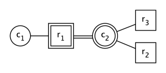
Figure 1: Vertices $r_{1}$ and $c_{2}$ are matched; others are not. Two augmenting paths starting from $c_{1}$ are possible.

Algorithm 3 gives the description of the Alternate function. This kernel alternates the matching edges with unmatching edges of the augmenting paths found; some of those paths end up being augmenting ones and some are only partially alternated. Here, each thread is assigned a number of rows. Since $rmatch$ of an unmatched row (that is also an endpoint of an augmenting path) has been set to $-2$ in the BFS kernel, only the threads whose row vertex’s match is $-2$ start Alternate. Since there might be several augmenting paths for an unmatched column, race conditions while writing on $cmatch$ and $rmatch$ arrays are possible. Such a race condition might cause infinite loops (inner while loop) or inconsistencies, if care is not taken. We prevent these by checking the predecessor of a matched row (line-8). For example, in Fig. 1, two different augmenting paths that end with $r_{2}$ and $r_{3}$ are found for $c_{1}$. If the thread of $r_{2}$ starts before the thread of $r_{3}$ in Alternate, the match of $c_{2}$ will be updated to $r_{2}$ (line-10). Then, $r_{3}$’s thread will read $matched\_row$ of $c_{2}$ as $r_{2}$ (line-7). This would cause an infinite loop without the check at line-8. Inconsistencies may occur when the threads of $r_{2}$ and $r_{3}$ are in the same warp. In this case, the if-check will not hold for both threads, and their row vertices will be written on $cmatch$ (line-10). Since only one thread will be successful at writing, this will cause an inconsistency. Such inconsistencies are fixed by FixMatching kernel which implements: $rmatch[r]\leftarrow-1$ for any $r$ satisfying $cmatch[rmatch[r]]\neq r$.

Algorithm 4 gives the description of a slightly different BFS kernel function. This function takes $root$ array as an extra argument. Initially, the root array is filled with $root[c]=0$ if $cmatch[c]>-1$, and $root[c]=c$ if $cmatch[c]=-1$. This array holds the root (as the index of the column vertex) of an augmenting path, and this information is transferred down during BFS. Whenever an augmenting path is found, the entry in $bfs\_array$ for the root of the augmenting path is set to ${\sc L_{0}}{}-2$. This information is used at the beginning of BFS kernel. No more BFS traversals is done, if an augmenting path is found for the root of the traversed column vertex. Therefore, while the method increases the global memory accesses by introducing an extra array, it provides an early exit mechanism for BFS.

Data: $bfs\_level,bfs\_array,cxadj,cadj,nc,rmatch,root$

             $vertex\_inserted,augmenting\_path\_found$

1

2$process\_cnt\leftarrow{\sc getProcessCount}(nc)$;

3 for $i$ from $0$ to $process\_cnt-1$ do

4       $col\_vertex\leftarrow i\times tot\_thread\_num+tid$;

5       if $bfs\_array[col\_vertex]$ $=$ $bfs\_level$ then

6             $myRoot\leftarrow root[col\_vertex]$;

7             if $bfs\_array[myRoot]<{\sc L_{0}}{}-1$ then

8                   $continue$;

9                  

10            for $j$ from $cxadj[col\_vertex]$ to $cxadj[col\_vertex+1]$  do

11                   $neighbor\_row\leftarrow cadj[j]$;

12                   $col\_match\leftarrow rmatch[neighbor\_row]$;

13                   if $col\_match>-1$ then

14                         if $bfs\_array[col\_match]$ $=$ ${\sc L_{0}}{}$ $-1$ then

15                               $vertex\_inserted\leftarrow{\bf true}$;

16                               $bfs\_array[col\_match]\leftarrow bfs\_level+1$;

17                               $root[col\_match]\leftarrow myRoot$;

18                               $predeccesor[neighbor\_row]\leftarrow col\_vertex$;

19                              

20                        

21                  else

22                         if $col\_match$=$-1$ then

23                               $bfs\_array[myRoot]\leftarrow{\sc L_{0}}{}-2$;

24                               $rmatch[neighbor\_row]\leftarrow-2$;

25                               $predeccesor[neighbor\_row]\leftarrow col\_vertex$;

26                               $augmenting\_path\_found\leftarrow{\bf true}$;

27                              

28                        

29                  

30            

31      

32

Algorithm 4 BFS Kernel Function-2 (GPUBFS-WR)

We further improve GPUBFS-WR by making use of the arrays $root$ and $bfs\_array$. BFS kernels might find several rows to match with the same unmatched column, and set $rmatch[\cdot]$ to $-2$ for each. These cause Alternate to start from several rows that can be matched with the same unmatched column. Therefore, it may perform unnecessary alternations, until these augmenting paths intersect. Conflicts may occur at these intersection points (which are then resolved with FixMatching function). By choosing ${\sc L_{0}}{}$ as 2, we can limit the range of the values that $bfs\_array$ takes to positive numbers. Therefore, by setting the $bfs\_array$ to $-(neighbor\_row)$ at line 19 of Algorithm 4, we can provide more information to the Alternate function. With this, Alternate can determine the beginning and the end of an augmenting path, and it can alternate only among the correct augmenting paths. APsB-GPUBFS-WR (and Alternate function used together) includes these improvements. However, they are not included in APFB-GPUBFS-WR since they do not improve its performance.

4 Experiments

The running time of the proposed implementations are compared against the sequential HK and PFP implementations [8], and against the multicore parallel implementations P-PFP, P-DBFS, and P-HK [1]. The CPU implementations are tested on a computer with 2.27GHz dual quad-core Intel Xeon CPUs with 2-way hyper-threading and 48GB main memory. The algorithms are implemented in C++ and OpenMP. The GPU implementations are tested on NVIDIA Tesla C2050 with usable 2.6GB of global memory. C2050 is equipped with 14 multiprocessors each containing 32 CUDA cores, totaling 448 CUDA cores. The implementations are compiled with gcc-4.4.4, cuda-4.2.9 and -O2 optimization flag. For the multicore algorithms, 8 threads are used. A standard heuristic (called the cheap matching, see [8]) is used to initialize all tested algorithms. We compare the running time of the matching algorithms after this common initialization.

Two different main algorithms APFB and APsB can use two different BFS kernel functions (GPUBFS and GPUBFS-WR). Moreover, each of these algorithms can have two versions (i) CT: uses a constant number of threads with fixed number of grid and block size ($256\times 256$) and assigns multiple vertices to each thread; (ii) MT: tries to assign one vertex to each thread. The number of threads used in the second version is chosen as $\mbox{MT}=\min(nc,\#threads)$ where $nc$ is the number of columns, and $\#threads$ is the maximum number of threads of the architecture. Therefore, we have eight GPU-based algorithms.

The algorithms are run on bipartite graphs corresponding to 70 different matrices from variety of classes at UFL matrix collection [6]. We also permuted the matrices randomly by rows and columns and included them as a second set (labeled RCP). These permutations usually render the problems harder for the augmenting-path-based algorithms [8]. For both sets, we report the performance for a smaller subset which contains those matrices in which at least one of the sequential algorithms took more than one second. We call these sets O_S1 (28 matrices) and RCP_S1 (50 matrices). We also have another two subsets called O_Hardest20 and RCP_Hardest20 that contain the set of 20 matrices on which the sequential algorithms required the longest running time.

Table 1: Geometric mean of the running time of the GPU algorithms on different sets of instances.

	APFB				APsB
	GPUBFS		GPUBFS-WR		GPUBFS		GPUBFS-WR
	MT	CT	MT	CT	MT	CT	MT	CT
O_S1	2.96	1.89	2.12	1.34	3.68	2.88	2.98	2.27
O_Hardest20	4.28	2.70	3.21	1.93	5.23	4.14	4.20	3.13
RCP_S1	3.66	3.24	1.13	1.05	3.52	3.33	2.22	2.14
RCP_Hardest20	7.27	5.79	3.37	2.85	12.06	10.75	8.17	7.41

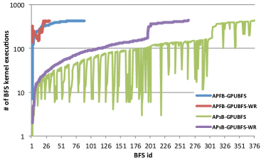
(a) Hamrle3

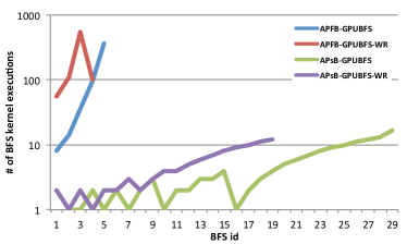
(b) Delanuay_n23

Figure 2: The BFS ids and the number of kernel executions for each BFS in APsB and APFB variants for two graphs. The $x$ axis shows the id of the while iteration at line 2 of APsB. The $y$ axis shows the number of the while iterations at line 6 of APsB.

First, we compare the performance of the proposed GPU algorithms. Table 1 shows the geometric mean of the running time on different sets. As we see from the table, using constant number of threads (CT) always increases the performance of an algorithm, since it increases the granularity of the work performed by each thread. GPUBFS-WR is always faster than GPUBFS. This is because of the unnecessary BFS traversals in the GPUBFS algorithm. GPUBFS cannot determine whether an augmenting path has already been found for an unmatched column, therefore it will continue to explore. This unnecessary BFS traversals not only increase the BFS time, but also reduce the likelihood of finding an augmenting path for other unmatched columns. Moreover, the Alternate scheme turns out to be more suitable for APFB than APsB, in which case it can augment along more paths (there is a larger set of possibilities). For example, Figs. 2(a) and 2(b) show the number of BFS iterations and the number of BFS levels in each iteration for, respectively, Hamrle3 and Delanuay_n23 graphs. As clearly seen from both of the figures, APFB variants converges in smaller number of iterations than APsB variants; and for most of the graphs, the total number of BFS kernel calls are less for APFB (as in Fig. 2(a)). However, for a small subset of the graphs, although the augmenting path exploration of APsB converges in larger number of iterations, the numbers of the BFS levels in each iterations are much less than APFB (as in Fig. 2(b)). Unlike the general case, APsB outperforms APFB in such cases. Since APFB using GPUBFS-WR and CT almost always obtains the best performance, we only compare the performance of this algorithm with other implementations in the following.

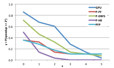
(a) Original graphs

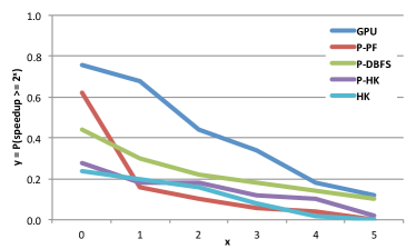
(b) Permuted graphs

Figure 3: Log-scaled speedup profiles.

Figures 3(a) and 3(b) give the log-scaled speedup profiles of the best GPU and multicore algorithms on the original and permuted graphs. The speedups are calculated with respect to the fastest of the sequential algorithms PFP and HK (on the original graphs HK was faster; on the permuted ones PFP was faster). A point $(x,y)$ in the plots corresponds to the probability of obtaining at least $2^{x}$ speedup is $y$. As the plots show, the GPU algorithm has the best overall speedup. It is faster than the sequential HK algorithm for $86\%$ of the original graphs, while it is faster than PFP on $76\%$ of the permuted graphs. P-DBFS obtains the best performance among the multicore algorithms. However, its performance degrades on permuted graphs. Although P-PFP is more robust than P-DBFS to permutations, its overall performance is inferior to that of P-DBFS. P-HK is outperformed by the other algorithms in both sets.

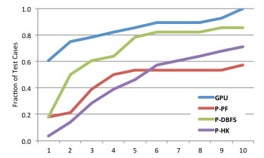
(a) Original graphs

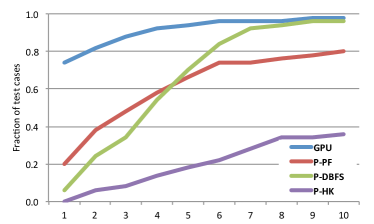
(b) Permuted graphs

Figure 4: Performance profiles

Figures 4(a) and 4(b) show the performance profiles of the GPU and multicore algorithms. A point $(x,y)$ in this plot means that with $y$ probability, the algorithm obtains a performance that is at most $x$ times worse than the best running time. The plots clearly show the separation among the GPU algorithm and the multicore ones, especially for original graphs and for $x\leq 7$ for the permuted ones, thus marking GPU as the fastest in most cases. In particular, GPU algorithm obtains the best performance in $61\%$ of the original graphs, while this ratio increases to $74\%$ for the permuted ones.

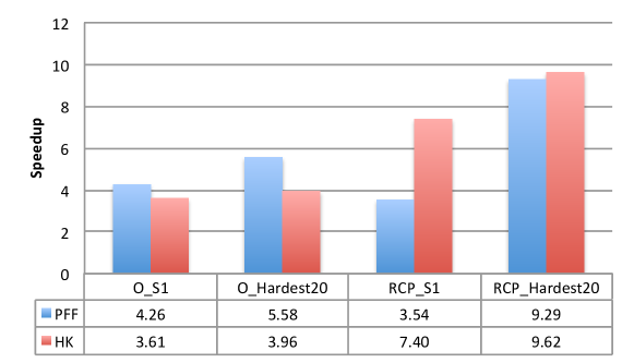
Figure 5: Overall speedup of the proposed GPU algorithm w.r.t. PFP (left bars) and HK (right bars) algorithms.

Figure 5 gives the overall speedups. The proposed GPU algorithm obtains average speedup values of at least $3.61$ and $3.54$ on, respectively, original and permuted graphs. The speedups increase for the hardest instances, where the GPU algorithm achieves $3.96$ and $9.29$ speedup, respectively, on original and permuted graphs. Table 2 gives the actual running time for O_Hardest20 sets for the best GPU and multicore algorithms, together with the sequential algorithms (the running time of all mentioned algorithms on the complete set of graphs can be found at http://bmi.osu.edu/hpc/software/matchmaker2/maxCardMatch.html). As seen from this table, except six instances among the original graphs and another two among the permuted graphs, the GPU algorithm is faster than the best sequential algorithm. It is also faster than the multicore ones in all, except five original graphs.

Table 2: The actual running time of each algorithm for the O_Hardest20 set.

	Original graphs				Permuted graphs
Matrix name	GPU	P-DBFS	PFP	HK	GPU	P-DBFS	PFP	HK
roadNet-CA	0.34	0.53	0.95	2.48	0.39	1.88	3.05	4.89
delaunay_n23	0.96	1.26	2.68	1.11	0.90	5.56	3.27	14.34
coPapersDBLP	0.42	6.27	3.11	1.62	0.38	1.25	0.29	1.26
kron_g500-logn21	0.99	1.50	5.37	4.73	3.71	4.01	64.29	16.08
amazon-2008	0.11	0.18	6.11	1.85	0.41	1.37	61.32	4.69
delaunay_n24	1.98	2.41	6.43	2.22	1.86	12.84	6.92	35.24
as-Skitter	0.49	1.89	7.79	3.56	3.27	5.74	472.63	29.63
amazon0505	0.18	22.70	9.05	1.87	0.24	15.23	17.59	2.23
wikipedia-20070206	1.09	5.24	11.98	6.52	1.05	5.99	9.74	5.73
Hamrle3	1.36	2.70	0.04	12.61	3.85	7.39	37.71	57.00
hugetrace-00020	7.90	393.13	15.95	15.02	1.52	9.97	8.68	38.27
hugebubbles-00000	13.16	3.55	19.81	5.56	1.80	10.91	10.03	38.97
wb-edu	33.82	8.61	3.38	20.35	17.43	20.10	9.49	51.14
rgg_n_2_24_s0	3.68	2.25	25.40	0.12	2.20	12.50	5.72	31.78
patents	0.88	0.84	92.03	16.18	0.91	0.97	101.76	18.30
italy_osm	5.86	1.20	1.02	122.00	0.70	3.97	6.24	18.34
soc-LiveJournal1	3.32	14.35	243.91	21.16	3.73	7.14	343.94	20.71
ljournal-2008	2.37	10.30	360.31	17.66	6.90	7.58	176.69	23.45
europe_osm	57.53	11.21	14.15	1911.56	7.21	37.93	68.18	197.03
com-livejournal	4.58	22.46	2879.36	34.28	5.88	17.19	165.32	29.40

5 Concluding remarks

We proposed a parallel BFS based GPU implementation of maximum cardinality matching algorithm for bipartite graphs. We presented experiments on various datasets, and compared the performance of the proposed GPU implementation against sequential and multicore algorithms. The experiments showed that the proposed GPU implementations are faster than the existing parallel multicore implementations. The speedups achieved with respect to well-known sequential implementations varied from $0.03$ to $629.19$, averaging $9.29$ on a set of 20 hardest problems with respect to the fastest sequential algorithm. A GPU is a restricted memory device. Although, an out-of-core or distributed-memory type algorithm is amenable when the graph does not fit into the device, a direct implementation of these algorithms will surely not be efficient. We plan to investigate the techniques to obtain good matching performance for extreme-scale bipartite graphs on GPUs.

References

- [1] Azad, A., Halappanavar, M., Rajamanickam, S., Boman, E.G., Khan, A., Pothen, A.: Multithreaded algorithms for maximum matching in bipartite graphs. In: 26th IPDPS. pp. 860–872. IEEE (2012)
- [2] Azad, A., Pothen, A.: Multithreaded algorithms for matching in graphs with application to data analysis in flow cytometry. In: 26th IPDPS Workshops & PhD Forum. pp. 2494–2497. IEEE (2012)
- [3] Berge, C.: Two theorems in graph theory. P. Natl. Acad. Sci. USA 43, 842–844 (1957)
- [4] Burkard, R., Dell’Amico, M., Martello, S.: Assignment Problems. SIAM, Philadelphia, PA, USA (2009)
- [5] Çatalyürek, U.V., Deveci, M., Kaya, K., Uçar, B.: Multithreaded clustering for multi-level hypergraph partitioning. In: 26th IPDPS. pp. 848–859. IEEE (2012)
- [6] Davis, T.A., Hu, Y.: The University of Florida sparse matrix collection. ACM T. Math. Software 38(1), 1:1–1:25 (2011)
- [7] Duff, I.S., Erisman, A.M., Reid, J.K.: Direct Methods for Sparse Matrices. Oxford University Press, London (1986)
- [8] Duff, I.S., Kaya, K., Uçar, B.: Design, implementation, and analysis of maximum transversal algorithms. ACM T. Math. Software 38(2), 13 (2011)
- [9] Duff, I.S., Wiberg, T.: Remarks on implementation of assignment algorithms. ACM T. Math. Software 14(3), 267–287 (1988)
- [10] Fagginger Auer, B., Bisseling, R.: A GPU algorithm for greedy graph matching. Facing the Multicore-Challenge II pp. 108–119 (2012)
- [11] Goldberg, A., Kennedy, R.: Global price updates help. SIAM J. Discrete Math. 10(4), 551–572 (1997)
- [12] Goldberg, A.V., Tarjan, R.E.: A new approach to the maximum flow problem. J. Assoc. Comput. Mach. 35, 921–940 (1988)
- [13] Hochbaum, D.S.: The pseudoflow algorithm and the pseudoflow-based simplex for the maximum flow problem. In: 6th IPCO, pp. 325–337. London, UK (1998)
- [14] Hopcroft, J.E., Karp, R.M.: An algorithm for maximum matchings in bipartite graphs. SIAM J. Comput. 2(4), 225–231 (1973)
- [15] John, P.E., Sachs, H., Zheng, M.: Kekulé patterns and Clar patterns in bipartite plane graphs. J. Chem. Inf. Comp. Sci. 35(6), 1019–1021 (1995)
- [16] Kaya, K., Langguth, J., Manne, F., Uçar, B.: Push-relabel based algorithms for the maximum transversal problem. Comput. Oper. Res. 40(5), 1266–1275 (2012)
- [17] Kim, W.Y., Kak, A.C.: 3-D object recognition using bipartite matching embedded in discrete relaxation. IEEE T. Pattern Anal. 13(3), 224 –251 (1991)
- [18] Vasconcelos, C., Rosenhahn, B.: Bipartite graph matching computation on GPU. In: Energy Minimization Methods in Computer Vision and Pattern Recognition. pp. 42–55. Springer (2009)