March 2013
Model–Independent Identification of Inelastic WIMPs
from Direct Dark Matter Detection Experiments
Sen Miao1,‡, Chung-Lin Shan2,§, and Yu-Feng Zhou1,¶
1
State Key Laboratory of Theoretical Physics,
Kavli Institute for Theoretical Physics China,
Institute of Theoretical Physics,
Chinese Academy of Sciences
Beijing 100190, China
2
Physics Division,
National Center for Theoretical Sciences
No. 101, Sec. 2, Kuang-Fu Road,
Hsinchu City 30013, Taiwan, R.O.C.
‡ E-mail: miaosen@itp.ac.cn
§ E-mail: clshan@phys.nthu.edu.tw
¶ E-mail: yfzhou@itp.ac.cn
Abstract
In this paper, we introduce model–independent data analysis procedures for identifying inelastic WIMP–nucleus scattering as well as for reconstructing the mass and the mass splitting of inelastic WIMPs simultaneously and separately. Our simulations show that, with observed WIMP signals from one experiment, one could already distinguish the inelastic WIMP scattering scenarios from the elastic one. By combining two or more data sets with positive signals, the WIMP mass and the mass splitting could even be reconstructed with statistical uncertainties of less than a factor of two.
1 Introduction
Different astronomical observations and measurements indicate that more than 80% of all matter in the Universe is dark (i.e. interacts at most very weakly with electromagnetic radiation and ordinary matter). The dominant component of this cosmological Dark Matter (DM) must be due to some yet to be discovered, non–baryonic particles. Weakly Interacting Massive Particles (WIMPs) arising in several extensions of the Standard Model of electroweak interactions are one of the leading DM candidates. Currently, the most promising method to detect different WIMP candidates is the direct detection of the recoil energy deposited in a low–background underground detector by scattering of ambient WIMPs off target nuclei (for reviews, see Refs. [1, 2, 3, 4, 5, 6]).
The first positive signal of WIMPs was reported by the DAMA Collaboration with observation of the annual modulation of the event rate of possible DM–target interaction by the DAMA/NaI detector [7] (for the latest updated results, see Refs. [8]). The CoGeNT Collaboration announced also their result with a modulated component of unknown origin [9, 10, 11]. The CRESST Collaboration published in 2011 their newest result with more observed events than expected backgrounds in the CRESST-II experiment [12]. However, other direct DM detection experiments can so far mostly observe only very few candidate events and a large part ( 40% to 60%) of these events would be unrejected backgrounds [13, 14, 15, 16, 17, 18].
Many theoretical scenarios have been proposed to find an explanation for reconciling all these results from different experiments with various target nuclei. Among them, one of the mostly discussed and experimentally constrained frameworks is inelastic Dark Matter (iDM) models [19, 20]. The basic assumption of iDM models is that the incident WIMPs scatter inelastically off target nuclei and then transit to a slightly heavier (exciting) state with a tiny mass (energy) splitting , while the elastic scattering channel is suppressed or forbidden. Due to the kinematics of inelastic scattering, the targets with heavier nuclei have greater sensitivities than those with lighter nuclei. This suggests that the signals reported by DAMA which utilises relatively heavy iodine nuclei may not be detected by other experiments with light target nuclei such as germanium and silicon. Comparisons between exclusion limits on the cross section versus mass (splitting) () planes in the iDM scenarios by using various experimental data have been done [21, 22]. In Ref. [22] the authors considered also the case of low–mass WIMPs ( 5 GeV) with a tiny mass splitting ( 10 keV). Meanwhile, a method for reconstructing the iDM parameters, most importantly the WIMP mass and the mass splitting , based on likelihood analysis has been suggested [23].
In the recent years, several experimental collaborations have (re)analyzed their (null) observation results and found severe constraints on the parameter space of iDM, i.e. on the mass splitting versus the WIMP mass plane. From these analyses, exclusion limits for mass splitting up to 250 keV in the mass range between 40 GeV and 1 TeV with different detector materials have been given [13, 24, 25, 26, 27, 18]. However, in all these works, data analyses have been done basically by estimations of the (differential) event rate, which is strongly halo–model dependent. In addition, types and (relative) strengths of different DM–nucleus (quark) interactions are important factors in direct and indirect DM detection experiments [1, 2].
Hence, in this paper, as complementarity and extension of our earlier work on developing methods for reconstructing WIMP properties in elastic scattering framework as model–independently as possible [28, 29, 30] we introduce new model–independent approaches for identifying inelastic WIMP–nucleus scattering scenarios as well as for reconstructing the most important properties of inelastic WIMPs: the mass and the mass splitting simultaneously and separately. Our method is based on an estimation of a characteristic energy corresponding to a threshold (minimal required) (one–dimensional) velocity of incident (inelastic) WIMPs, .111 Note that, in conventional elastic scattering framework, all incident WIMPs with non–zero velocity could scatter off target nuclei and deposit recoil energies . This means that for elastic WIMPs and for inelastic WIMPs. In fact, later we will show that the characteristic energy is proportional to the mass splitting . This can be done by determining the maximum of the integral over the one–dimensional velocity distribution function of incident WIMPs. Once this characteristic energy can be solved by using data sets of positive (inelastic) WIMP signals with different target nuclei, one can then determine the (degenerate) WIMP mass and the tiny mass splitting straightforwardly.
The remainder of this paper is organized as follows. In Sec. 2, we develop the formalism of the methods for reconstructing the one–dimensional WIMP velocity distribution function, determining the WIMP mass and the mass splitting as well as estimating the characteristic energy and in turn identifying the inelastic WIMP–nucleus scattering scenarios. In Sec. 3, we demonstrate the ability and shortcomings of our model–independent methods by presenting numerical results based on Monte–Carlo simulations. The possibility of distinguishing the inelastic WIMP scenarios from the elastic one will be particularly discussed. We conclude in Sec. 4. Some technical details for our analysis will be given in the appendices.
2 Formalism
In this section, we develop the formulae needed in our model–independent reconstructions of different properties of halo WIMPs in iDM scenarios, both of an approximated analytic method and an iterative numerical procedure will be considered.
We start with the basic expression for the differential event rate for (elastic) WIMP–nucleus scattering given by [1]:
| (1) |
Here is the direct detection event rate, i.e. the number of events per unit time and unit mass of detector material, is the energy deposited in the detector, is the (elastic) nuclear form factor, is the one–dimensional velocity distribution function of the WIMPs impinging on the detector, is the absolute value of the WIMP velocity in the laboratory frame. The constant coefficient is defined as
| (2) |
where is the WIMP density near the Earth and is the total cross section ignoring the form factor suppression. The reduced mass is defined by , where is the WIMP mass and that of the target nucleus. Finally, is the minimal incoming velocity of incident WIMPs that can deposit the energy in the detector:
| (3) |
with the transformation constants
| (4) |
and
| (5) |
is the maximal WIMP velocity in the Earth’s reference frame, which is related to the escape velocity from our Galaxy at the position of the Solar system, km/s.
2.1 Reconstruction of the velocity distribution
Following the process in Ref. [28], we define
| (6) |
Eq. (1) can then be rewritten as222 For simplicity, we set at first here the maximal cut–off of the one–dimensional WIMP velocity distribution as infinity. Later we will discuss correction of the formulae given here in the practical use with real (generated) data events.
| (7) |
Since WIMPs in today’s Universe move quite slow, must vanish as approaches infinity: . Thus and in turn approaches a finite value. Differentiating both sides of Eq. (7) with respect to and using Eq. (3), we can find
| (8) |
Here, from the definition (3) of , we can firstly find that
| (9) |
and an analytic expression of can be solved from the definition (3) directly as:
| (10) |
Note that, corresponding to one specific value of , there are two possible values of , except of
| (11) |
Here is the threshold (minimal required) velocity of incident inelastic WIMPs, which can produce recoil energy at all.
Since the expression (8) of holds for arbitrary , we can write down the following result directly:
| (12) |
with
| (13) |
Although the right–hand side of this expression depends on the as yet unknown constant , is the normalized velocity distribution, i.e. it is defined to satisfy: . Therefore, the normalized one–dimensional velocity distribution function of inelastic WIMPs can be given by
| (14) |
with the normalization constant :
| (15) |
Note that, for the case of elastic WIMP–nucleus scattering, , the expressions (14) and (15) can then be reduced to the simple, analytic forms given in Eqs. (12) and (13) of Ref. [28].
2.2 Determinations of the WIMP mass and the mass splitting
The expression for reconstructing the one–dimensional velocity distribution of inelastic WIMPs given in Eqs. (14) and (15) can unfortunately not be used directly, since at first there are two unknowns, i.e. the WIMP mass (involved in ) and the mass splitting (involved in ). Moreover, the typical peaky shape of the recoil spectrum of inelastic WIMPs (see e.g. Figs. 1 to 4) makes its reconstruction more complicated and therefore a similar development of procedures introduced in Refs. [28, 29] is basically impossible.
Hence, in this subsection, we introduce a new approach for determining the WIMP mass and the mass splitting based on the estimation of the characteristic energy , which requires the reconstruction of the peaky inelastic WIMP recoil spectrum.
2.2.1 Determinations of and
From the definition (3) of , one have
| (16) |
Then the characteristic energy corresponding to the minimal value of , , can easily be solved as
| (11) |
which is proportional to the mass splitting and the proportionality constant is simply a function of the WIMP mass . Hence, by combining two experimental data sets with different target nuclei, and , one can derive analytic expressions for determining and as functions of the characteristic energy and :
| (17) |
and
| (18) |
Then, since are two independent variables, by using the standard Gaussian error propagation, the statistical uncertainties on the reconstructed and can be given as
| (19) | |||||
and
| (20) | |||||
2.2.2 Ansatz for reconstructing the inelastic–scattering recoil spectrum
Note that, for the use of Eqs. (17) and (18), one needs to estimate the characteristic energy corresponding to the threshold (minimal required) velocity of incident inelastic WIMPs , which could produce recoil energy at all. This means that is the lowest bound of the velocity of inelastic WIMPs, which could contribute to the integral over the one–dimensional velocity distribution function on the right–hand side of Eq. (1). This means in turn that the integral over , or, equivalently, a “reduced” differential event rate (i.e. the differential event rate divided by the squared nuclear form factor):
| (21) |
should be maximal once .
On the other hand, for the simplest isothermal spherical halo model, the normalized one–dimensional velocity distribution function can be expressed as [28]:
| (22) |
where km/s is the Sun’s orbital speed around the Galactic center. More realistically, by taking into account the orbital motion of the Solar system around the Galaxy, the more frequently used shifted Maxwellian velocity distribution has been given by [28]:
| (23) |
where is the time–dependent Earth’s velocity in the Galactic frame:
| (24) |
where June 2nd is the date on which the Earth’s velocity relative to the WIMP halo is maximal.
Substituting these two expressions into Eq. (1) and using Eq. (3), one can easily obtain that333 As in Sec. 2.1, we assume here that the cut–off on , , as well as the experimental maximal cut–off energy are large enough and the integral in the higher velocity/energy range can be neglected.
| (25a) |
and
| (25b) |
Then, similar to the use of the exponential approximation for reconstructing the recoil spectrum of elastic WIMP–nucleus scattering [28], in order to approximate the measured recoil spectrum and take into account the extra contribution predicted in inelastic WIMP scattering scenarios, we introduce empirically here
| (26) |
where
| (27) |
with the total WIMP signal events in our data set and the experimental exposure ; and are two fitting parameters which we want to estimate by using the measured recoil energies directly. By using the ansatz (26), the position of the peak of the inelastic recoil spectrum can be solved easily and then estimated by (mathematical details are given in Appendix A.2)
| (28) |
with the statistical uncertainty given by
where the th momentum of the recoil energy spctrum can be estimated by
| (30) |
Note that we assumed here (unrealistically) that the minimal experimental cut–off energy is negligible and the maximal one is infinity (a numerical correction will be discussed in the next subsection). Finally, two fitting parameters in the ansatz (26) can be estimated separately as
| (31a) |
and
| (31b) |
By using the approximation (26), the expression (14) for reconstructing the one–dimensional WIMP velocity distribution can be rewritten as
| (32) | |||||
with the normalization constant given in Eq. (15). Note that, for reconstructing by using Eqs. (32) and (15), the constant in Eq. (27) can be cancelled out, since this appears in both of the expression (14) or (32) and the expression (15).
On the other hand, as discussed at the beginning of this subsection, is the lowest bound of the integral in Eqs. (1) or (21), which gives a maximal value of the (reduced) event rate and thus have to satisfy the following condition:
| (33) |
By using the ansatz (26) for reconstructing the inelastic scattering spectrum, one can find that
| (34) |
can then be solved numerically and the statistical uncertainty on can be estimated by
| (35) | |||||
Here we have
| (36) |
and for are given in Appendix C. Note that, for the analytic estimates of and given by Eqs. (31a) and (31b), one has
| (37) |
2.3 A numerical correction
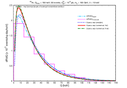
By using Eqs. (30), (31a) and (31b) to estimate the spectrum fitting parameters and analytically, one has to assume that the (experimental) minimal cut–off energy should be negligibly small () and the maximal one large enough ( a few hundred keV). This would still be a challenge for next–generation detectors. Moreover, due to the local escape velocity of halo WIMPs , or, equivalently, the maximal cut–off on its one–dimensional velocity distribution , there are not only a kinematic maximal but also a minimal cut–off energies, below and above which the incident WIMPs could produce recoil energies in our detector (see e.g. Figs. 4). From Eq. (13), one can get
| (38a) |
and
| (38b) |
As shown later in Sec. 3, this could be a serious issue once the mass splitting 30 keV, especially for light target nuclei, i.e. and (see Figs. 4).
Moreover, as we will show in Sec. 3.3, for larger WIMP masses ( 200 GeV), the reconstructed WIMP mass could be strongly underestimated: the larger the mass splitting, the worse the mass reconstruction. Hence, we introduce in this subsection an iterative process for correcting the estimation of the fitting parameters, and , in the hope that this correction could reduce the systematic deviation of the solved and thereby alleviate the underestimation of the reconstructed WIMP mass.
We start from Eq. (30). Define
| (39) |
where are given in Eqs. (A17) to (A18c) in Appendix A.2. In stead of defined on the left–hand side of Eq. (30), defined above should be more suitable to be estimated by the average value of the summation over all measured recoil energies in the th power given on the right–hand side of Eq. (30). Thus one has
| (40) |
By setting estimated by Eqs. (31a) and (31b), one can solve numerically, denoted by , by using the expressions of , and , simultaneously444 The detailed description about solving and from and simultaneously will be given in Appendix B. .
Note that expressions (32) and (34) for reconstructing the one–dimensional WIMP velocity distribution and solving the characteristic energy can be used by substituting both the analytic and numerical estimations of the fitting parameters and , whereas for using Eq. (35) to estimate the statistical uncertainty on solved with the numerically estimated and , the summation runs only for and .
3 Numerical results
In this section, we present numerical results of the reconstruction of the recoil spectrum, the identification of the positivity of (as the check of the iDM scenarios) as well as the reconstruction of the WIMP mass and the mass splitting based on Monte–Carlo simulations. The special case of zero mass splitting , i.e. the case of elastic WIMP scattering, will be particularly discussed at the end of this section as a demonstration of the usefulness of our model–independent approach for distinguishing the inelastic WIMP scenarios from the elastic one.
For generating WIMP–induced signals in our simulations, we use the shifted Maxwellian velocity distribution given in Eq. (23) with the Sun’s Galactic orbital velocity km/s; the time dependence of the Earth’s velocity in the Galactic frame has been ignored, i.e. is used. Moreover, the maximal cut–off of the one–dimensional WIMP velocity distribution has been set as km/s. Meanwhile, the WIMP–nucleon cross section has been assumed to be only spin–independent (SI), pb, and the commonly used analytic form for the elastic nuclear form factor
| (41) |
has been adopted. Here is the recoil energy transferred from the incident WIMP to the target nucleus, is a spherical Bessel function, is the transferred 3-momentum, for the effective nuclear radius we use with and a nuclear skin thickness . In addition, the experimental threshold energies have been assumed to be negligible () and the maximal cut–off energies are set as keV for all target nuclei555 Note that, although we assume here (unrealistically) that one could experimentally measure recoil energies between and keV, since the effect of the kinematic maximal and minimal cut–off energies has been taken into account in our simulations, we only generate events between and the smaller one between and and then analyze the data sets numerically with these two cut–offs. . 5,000 experiments with 50 total events on average in one experiment have been simulated.
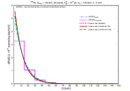
3.1 Reconstructing the recoil spectrum
In this subsection, we consider at first the reconstruction of the recoil spectrum, which is approximated by Eq. (26) with the fitting parameters and , as well as the estimation of the characteristic energy .
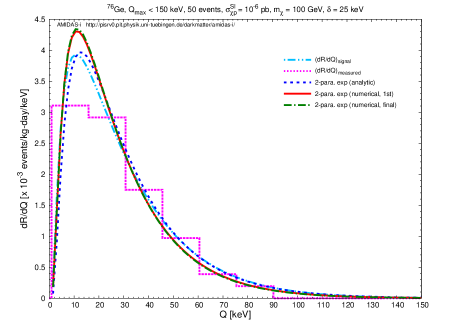
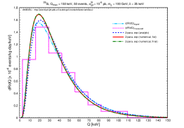
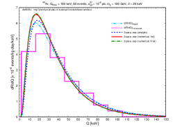
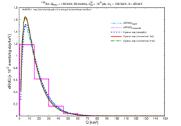
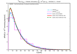
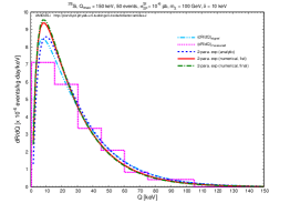
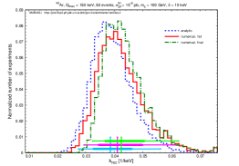
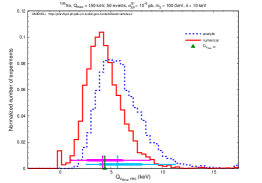
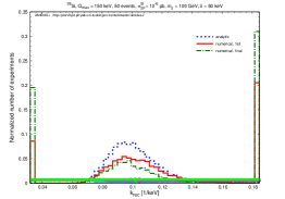
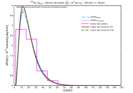
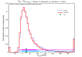
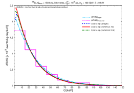
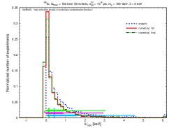
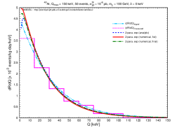
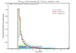
The top–left frame of Figs. 1 shows the measured recoil energy spectrum (dotted magenta histogram) for a target. The dash–double–dotted cyan curve is the inelastic WIMP–nucleus scattering spectrum used for generating recoil events. The input WIMP mass and mass splitting are set as GeV and keV. We show here also the reconstructed recoil spectra: while the dashed blue curve is the 2-parameter exponential spectrum (26) with the parameters and estimated analytically by Eqs. (31a) and (31b)666 For the analytically reconstructed spectrum shown here, the constant in Eq. (26) has been estimated by Eq. (27), in which the lower and upper bounds of the integral in the denominator have to be set as and . Then Eq. (27) can be rewritten as (42) where is the modified Bessel function of the second kind of order 1. Detailed derivation can be found in Appendix A.1. , the solid red and dash–dotted green curves are given with the parameters and estimated by the numerical method introduced in Sec. 2.3; the former and later show the results obtained from the first and final rounds of the iterative process777 Note that, as we will discuss later, the results given by our iterative numerical procedure might diverge (deviate larger and larger from the theoretical values) round by round. Thus, once the results given by the th run is too far away from the th run, our program will take the results of th run as the final results. This means that in some of the 5,000 simulated experiments the results of the final round are just those of the first or the second rounds. Note also that, because of the same divergency problem and of that the results given by the later round might not be much better than those of the first round, for the reconstructions of as well as the WIMP mass and the mass splitting shown later, we use only the results ( and ) given by the first round. .
()
()
()
()

()

()

()

()


()


()

()
It can be found that, firstly, the recoil spectra reconstructed numerically could really be the better approximations of the original theoretical spectrum, at least in the sense that the peaks of these spectra coincide very well. Secondly, and not really as expected, although the numerically reconstructed recoil spectra could be the better results than the analytically reconstructed one, the iterative procedure could not improve the correction further: only in a small part of the simulated experiments (shown here and later with different initial setup) the results coming from the second (and also the final) rounds could be clearly better than those coming from the first round; in most part of simulations there would no (significant) difference between the results given by different rounds, or those from the later round could even be worse…
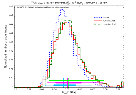
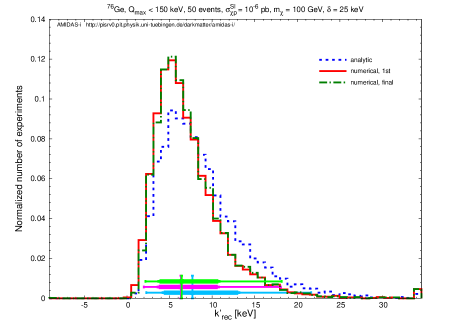
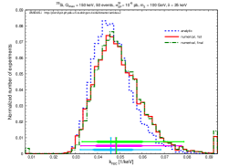
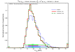
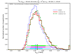
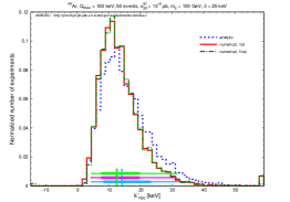
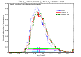
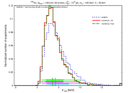
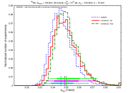
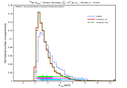
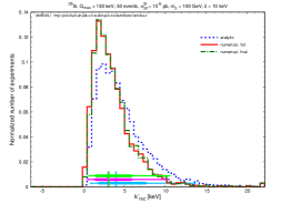
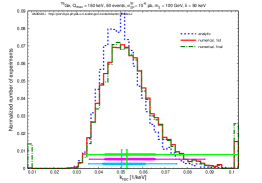
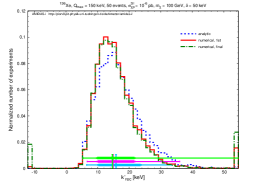
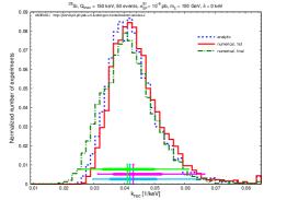
Moreover, in the top–right and bottom–left frames of Figs. 1, we show the distributions of the reconstructed fitting parameters and , respectively: while the dashed blue curves show the distributions of and estimated analytically by Eqs. (31a) and (31b), the solid red and dash–dotted green curves are those of the numerically estimated and , the former and later show the results given by the first and final rounds of the iterative process. Meanwhile, the cyan (magenta, light green) vertical lines indicate the median values of the simulated results (corresponding to the blue, red and green histograms), whereas the horizontal thick (thin) bars show the 1 (2) ranges of the results888 Here the 1 (2) ranges mean that 68.27% (95.45%) of the reconstructed values in the simulated experiments are in these ranges (central interval). .
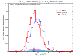
The top–right frame of Figs. 1 shows that the distributions of the reconstructed fitting parameter by both of the analytic and numerical methods are indeed basically Gaussian (with small tails in the high– range). Meanwhile, in the bottom–left frame the distributions of the reconstructed by both methods would be Gaussian distributions with a cut–off. Note that, is basically proportional to the square of the mass splitting, , (see Eq. (25a) and then Eq. (5)). The observation of the positively reconstructed indicates that our model–independent reconstruction proposed here should be useful and sensitive for identifying the inelastic WIMP–nucleus scattering scenarios.
Moreover, these two plots show also that there are neither significant differences between the median values of and (and thus the reconstructed recoil spectra) estimated in the first and final rounds of the numerical procedure, nor those between the distributions of them in the simulated experiments. In contrast, the differences between the numerical results and the analytic ones are clear. Hence, later we show only results given by the first round of the iterative process as the numerical reconstruction.
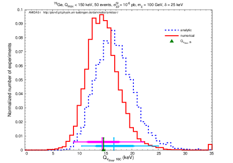
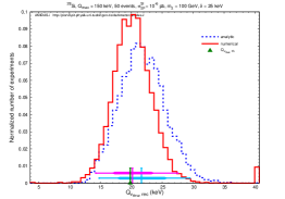
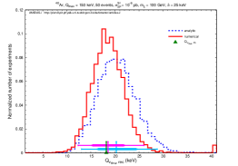
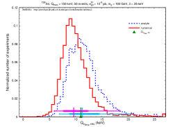
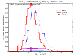
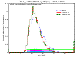
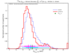
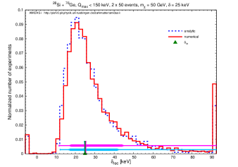
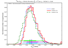
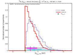
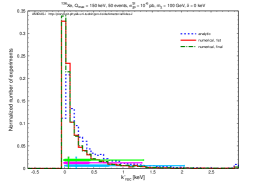
Finally, in the bottom–right frame of Figs. 1, we show the distributions of the characteristic energy solved by Eq. (34) with and estimated analytically (dashed blue) and numerically (solid red), respectively. The green vertical line given additionally here indicates the theoretical value of estimated by Eq. (11), . This plot shows that, firstly, both of the distributions of solved analytically and numerically are still basically Gaussian. Secondly, the median value of the numerically solved is indeed much closer to the theoretical estimate with a smaller 1 (2) upper and lower statistical uncertainties (and however a little bit longer tail in the high–energy range).
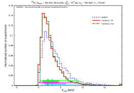
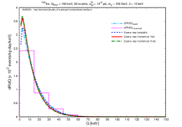
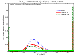
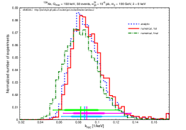
Considering the currently running and built/planned next–generation detectors, in Figs. 2 we present the results with several different target nuclei: (top), (middle) and (bottom). Basically, all observations discussed above hold, except that the median value of the analytically solved with the target is now closer to the theoretical estimate.
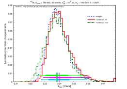
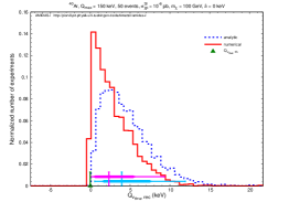
In Figs. 3 we consider a smaller mass splitting keV. For this extreme case999 The special case of (elastic WIMP–nucleus scattering) will be discussed particularly at the end of this section. , firstly, the tails of the distributions of , and solved analytically and numerically found in Figs. 1 and 2 are reduced significantly. This indicates that, for smaller mass splittings, the statistical fluctuations of , and given by both of the analytic and numerical methods would in principle be smaller. However, while there is still no significant difference between the numerically estimated from different rounds of the iterative procedure (the third column), the estimations of the fitting parameter (the second column) become clearly worse (and worse). This causes in turn larger deviations of the reconstructed recoil spectrum (see the first column).
Moreover, in all four plots of the distribution of the solved (forth column), an excess around can be seen clearly. This is caused by our setup of a lower bound used in solving and means thus that there is a small (but non–zero) possibility of obtaining non–physically negative , once the mass splitting is pretty small.
Here we would like to remind that, as shown in the first and forth columns of Figs. 3, since is proportional to the mass splitting (for a fixed WIMP mass , see Eq. (11)), once the mass splitting is quite small ( 10 keV), the position of the peak of the recoil spectrum, (a little bit smaller than ), would also be pretty small, probably smaller than the experimental minimal (software or even hardware) cut–off energy101010 For very light target nuclei, e.g. , is a little bit higher. Thus detectors with such materials would be more suitable for identifying low– inelastic WIMPs [31, 32, 33, 34, 35]. . In this case, the measured WIMP (inelastic) scattering spectrum (above the analysis threshold energy) would be monotonically decreased with increasing recoil energy and thus (very) difficult to be distinguished from the exponential–like elastic scattering spectrum (see e.g. the bottom–left frame of Figs. 2 and the left column of Figs. 3). Hence, a reduction of the threshold energy to be small enough/negligible would be necessary111111 So far, the minimal cut–off energies in most currently running experiments with semiconductor or liquid nobel gas detectors have been reduced to between 5 and 20 keV [27, 14, 12, 17, 16, 8, 36, 37, 38], whereas the threshold energy of the CoGeNT p–type point contact Ge detector can be down to as low as 2 keV ( 0.5 ) [10]. Meanwhile, the CDMS Collaboration developed new low–threshold technique, which can lower the analysis thresholds of their Ge and Si detectors to be smaller than 2 keV [39]. . Once this requirement can be achieved, our simulations shown here and in the next subsections indicate the possibility of a model–independent identification of inelastic WIMPs for a small mass splitting of keV.
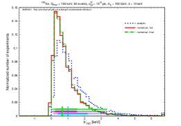
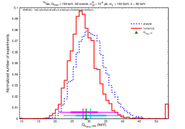
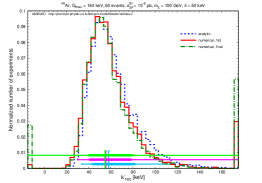
As comparison, in Figs. 4 a larger mass splitting keV is used. For this (relatively) high– case, the effect of the kinematic minimal and maximal cut–off energies (given in Eqs. (38a) and (38b)) becomes serious, especially for lighter target nuclei, e.g. (second row). In this case the analytic results seem to be more reliable; the tails of the distributions of the reconstructed , and offered by the numerical iterative procedure in high– (and even low–)value ranges become much longer and the divergency of the results mentioned earlier becomes now more problematic. Only numerical results offered from experiments with heavy target nuclei, e.g. and , could be used as auxiliary. Note here that the small bump of the distribution of reconstructed with the nucleus (forth frame in the bottom row) between 30 and 35 keV is caused by the (first) zero pont of the used nuclear form factor given in Eq. (41).
3.2 Identifying the positivity of


()

()

()
In this subsection, we study the positivity of the reconstructed characteristic energy (as the most important criterion of the identification of inelastic WIMP–nucleus scattering) in details.
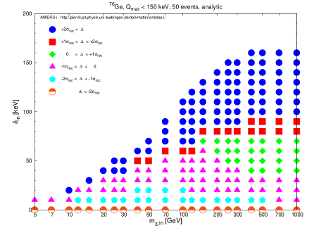
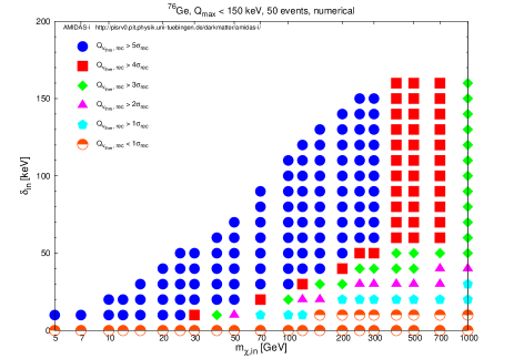
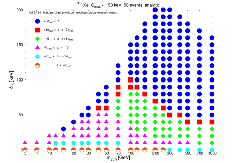
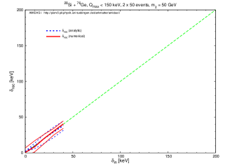
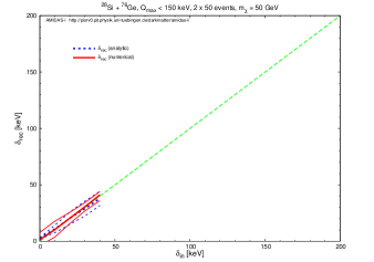
In the left frame of Figs. 5, we show the confidence levels (CLs) of the positivity of the analytically reconstructed (reconstructed in units of the estimated 1 lower statistical uncertainties ): CL (blue filled circles), CL (red filled squares), CL (green filled diamonds), CL (magenta filled up–triangles), CL (cyan filled pentagons), CL (orange up–half–filled circles). Here we use as the target nucleus and check 21 different input WIMP masses between 5 GeV and 1 TeV with 21 different input mass splittings between 0 and 200 keV. Note that the empty areas on the upper part of these plots indicate that the ability for reconstructing the fitting parameters and and then for solving would be limited by the kinematic minimal and maximal cut–off energies given in Eqs. (38a) and (38b), since either the WIMP mass is too small or the mass splitting is too large. It can be found here that, for WIMP masses 150 GeV (with as the target nucleus), the analytically reconstructed should in principle be at least 5 CL apart from zero; for larger masses 200 GeV 1 TeV, should still be CL apart from zero.
However, as shown in the previous subsection, the (analytically) reconstructed would be either overestimated (for smaller ) or underestimated (for larger ). Hence, in the right frame of Figs. 5 we also check the deviations of the analytically reconstructed from the theoretical values () in units of the estimated 1 lower statistical uncertainties : (blue filled circles), (red filled squares), (green filled diamonds), (magenta filled up–triangles), (cyan filled pentagons), (orange up–half–filled circles). It can be found that, firstly, for WIMP masses 50 GeV (with as the target nucleus), the analytically reconstructed would be overestimated (), once the mass splitting 40 keV; this upper bound could be reduced to 30 keV for heavier WIMP masses ( 300 GeV). Secondly, for cases of the non–zero mass splitting (), the deviations would in principle be maximal 2 or less than 1 overestimated ().
Now, by combining results showing in two frames of Figs. 5, one could conclude that, although the analytically reconstructed could be overestimated, with around 50 total events one could in principle already identify the positivity of with a high (3 to 5) confidence level, except of the (elastic WIMP scattering) case. This observation can in turn be used for distinguishing the inelastic WIMP–nucleus scattering scenarios from the elastic one.
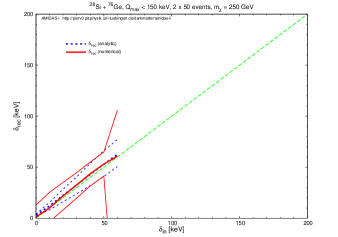
As comparison, in Figs. 6, we show the confidence levels of the positivity as well as the deviations of the numerically reconstructed with as the target nucleus. As shown in Figs. 1, 3 and 4, the statistical uncertainty on the numerically reconstructed as well as itself would in principle be smaller than the (uncertainty on the) analytically reconstructed one. Hence, firstly, for WIMP masses 300 GeV, the numerically reconstructed could be 5 CL apart from zero; for larger masses 300 GeV 1 TeV, could still be 4 CL apart from zero. Meanwhile, in the right frame it can be seen clearly that the boundary line between over– and underestimations of is reduced to 30 keV (for lighter WIMPs 100 GeV) to 20 keV (for heavier WIMPs 100 GeV).
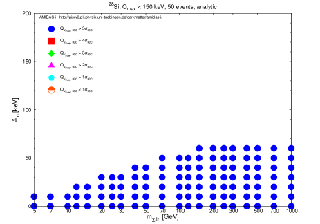
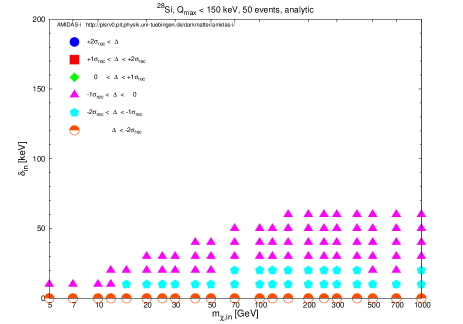
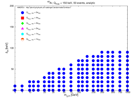
Moreover, in Figs. 7 we check the confidence levels of the positivity as well as the deviations of the analytically121212 Since, as discussed in the previous subsection, the analytically reconstructed fitting parameters and as well as the further solved would in principle be more reliable for higher mass splittings. reconstructed with (top), (middle) and (bottom) as detector materials. Although results offered by using light target nuclei, e.g. Si and Ar, would (almost) always be overestimated, an at least difference between reconstructed and zero could still be observed. Meanwhile, by using heavier nuclei, e.g. Xe, one could not only test a wilder area on the plane but also give results with a higher confidence level.
3.3 Determining
In this subsection, we present the simulation results of the reconstruction of one of the key properties of inelastic WIMPs, i.e. the WIMP mass .131313 Note that in all simulations shown in this and the next subsection, we always reconstruct the parameters and simultaneously in each simulated experiment. This means that neither nor has been fixed (as the input value) in our data analysis procedure.
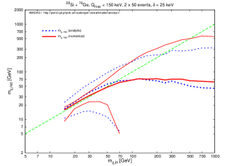
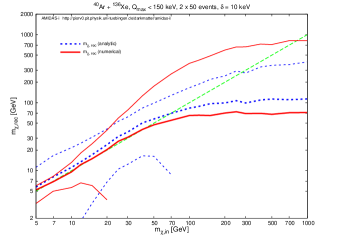
In the left frame of Figs. 8, we show the reconstructed WIMP mass estimated by Eq. (17) and the lower and upper bounds of the 1 statistical uncertainty estimated by Eq. (19) as functions of the input WIMP mass for the case of keV by using and as two target nuclei141414 From our results shown in Figs. 5 to 7, it seems that the WIMP mass (and the mass splitting) would be reconstructed better by combining two heavy target nuclei. However, our simulations show that, in practice, a combination of one light and one heavy target nucleus should be more suitable for reconstructing the WIMP mass. This can be understood as follows. The estimator given in Eq. (17) (Eq. (18)) of the (statistical uncertainty on the) reconstructed WIMP mass is inversely proportional to the (squared) difference between the characteristic energies of the recoil spectrum of two target nuclei (multiplied by the atomic mass of each nucleus). Hence, since the difference between the characteristic energies of the recoil spectrum of two heavy target nuclei is (much) smaller than that of one light and one heavy target nucleus, the statistical fluctuation caused by the use of only a few tens events (from one data set) would affect strongly our estimation of the (median values of the) reconstructed results, especially for heavier WIMP masses ( 40 GeV). with 50 total events on average in each data set. The dashed blue curves indicate the 1 band given with the parameters and estimated analytically by Eqs. (31a) and (31b), whereas the solid red curves indicate the band given with the numerically estimated and .
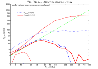


( keV)

( keV)
It can be seen that, firstly, for input WIMP masses 20 GeV GeV, while the analytically reconstructed WIMP mass (dashed blue) could be a bit overestimated, one could in principle reconstruct by the numerical method (solid red) pretty well. However, for heavier WIMP masses 70 GeV GeV, reconstructed by both methods would be (strongly) underestimated. Nevertheless, the 1 upper bound could still cover the input (true) value and therefore offer at least an upper constraint on the mass of inelastic WIMPs.
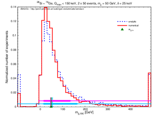
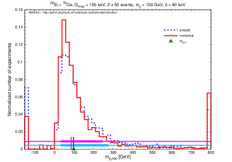
Meanwhile, in the middle frame of Figs. 8 we show the distributions of the reconstructed WIMP masses with analytically (dashed blue) and numerically (solid red) estimated and . While the cyan (magenta) vertical lines indicate the median values of the simulated results (corresponding to the blue and red distribution histograms) and the horizontal thick (thin) bars show the 1 (2) (68.27% (95.45%)) ranges of the results, the green vertical line indicates the true (input) WIMP mass of GeV. This plot shows that, for input WIMP masses 20 GeV GeV, the reconstructed WIMP masses should be concentrated around the true (input) value with tails in the high–mass range. However, it has also been found that, once the WIMP mass is heavy ( 100 GeV), the distributions of the reconstructed could extend pretty widely (not only to the high– range, but also to the unphysical, negative range).
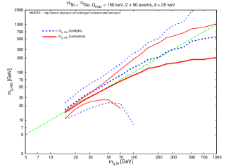
On the other hand, in contrast to a wide spread of the distribution of the reconstructed , the distribution of the reconstructed has been found to in principle be concentrated and converged around the theoretical value. Therefore, in the right frame of Figs. 8 we show the reconstructed WIMP mass and the 1 statistical uncertainty bands given by the median values of the reconstructed with and estimated analytically (dashed blue) and numerically (solid red), respectively. This plot shows that estimated by Eq. (17) with the median values of the reconstructed by using several data sets (with the same target nuclei) could indeed be (much) better than the median values of reconstructed by Eq. (17) with each single pair of data sets, especially for heavier input WIMP masses ( 100 GeV).
As comparison, in Figs. 9 we consider the case of a smaller mass splitting of keV (upper) and that of a larger one of keV (lower). The left frame in the upper row of Figs. 9 indicates that, while one could reconstruct the WIMP mass pretty well by both of the analytic and numerical methods for light WIMP masses ( GeV), for heavier WIMP masses ( GeV), the reconstructed would be (strongly) underestimated. Fortunately, a 1 upper bound as a constraint on the mass of inelastic WIMPs could still be given.
The middle frame in the upper row of Figs. 9 shows that, (only) for available WIMP mass range ( a few ), the distribution of the reconstructed could in principle be concentrated around the true (input) value, with however tails in the high– and negative–mass ranges. Moreover, the right frame shows that, for lighter mass splitting (e.g. keV shown here), reconstructed by using the median values of could also be (much) better than the median values of reconstructed with each single pair of data sets, up to even heavier WIMP mass of 1 TeV.
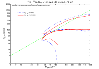
On the other hand, the lower row of Figs. 9 shows that, once the mass splitting 40 keV, except of the mass range between 40 GeV and 120 GeV, the distribution of the reconstructed WIMP mass could spread pretty widely and the reconstructed could anyway be (strongly) underestimated.
Generally speaking, for the reconstruction of the WIMP mass by using the target combination of and , our simulations show that, for mass splittings 40 keV, one could in principle reconstruct the WIMP mass in the range between and pretty precisely with a statistical uncertainty of 30% (for ) to a factor of 2 ().
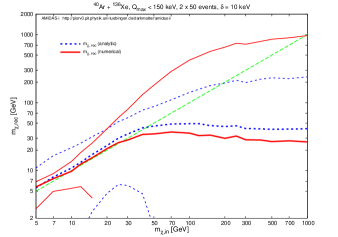
Finally, in Figs. 10 we present our simulation results of the reconstruction by using the combination of and as our target nuclei. Here we show only the case of a light mass splitting of keV. It has been found interestingly and a bit unexpectedly that, by using the target combination of and the strong underestimation of the reconstructed WIMP mass in the high–mass range could be alleviated with a much smaller statistical uncertainty (left) and the distribution of the reconstructed would also be more concentrated (middle).
3.4 Determining
In this subsection, we present the simulation results of the reconstruction of the second key property of inelastic WIMPs, i.e. the mass splitting .
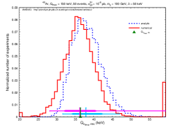
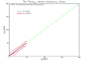
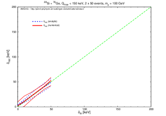
In the left frame of Figs. 11, we show the reconstructed mass splitting estimated by Eq. (18) and the lower and upper bounds of the 1 statistical uncertainty estimated by Eq. (20) as functions of the input mass splitting for the case of GeV by using and as two target nuclei with 50 total events on average in each data set. The dashed blue curves indicate the 1 band given with the parameters and estimated analytically by Eqs. (31a) and (31b), whereas the solid red curves indicate the band given with the numerically estimated and .

( GeV)

( GeV)
It can be seen that, firstly, due to the maximal kinematic cut–off energy in Eq. (38b), one could reconstruct the mass splitting only up to 50 keV (for a WIMP mass of 100 GeV). However, the middle frame of Figs. 11 shows that, once this reconstruction is achievable, the mass splitting could in principle be reconstructed pretty well: not only the median values of reconstructed both analytically and numerically could match the true (input) one, but also the distribution of the reconstructed would be pretty concentrated. Moreover, the middle frame of Figs. 11 shows also that a 3 to 5 ( 99%) CL of the positivity of the reconstructed mass splitting (as the confirmation of the inelastic WIMP scattering) could in principle be identified.
Finally, as in Figs. 8, in the right frame of Figs. 11 we show the reconstructed mass splitting and the 1 statistical uncertainty bands given by the median values of the reconstructed with and estimated analytically (dashed blue) and numerically (solid red), respectively. Not surprisingly, estimated by Eq. (18) with the median values of the reconstructed could be so good as the median values of reconstructed by Eq. (18) with each single pair of data sets; the former could have little bit smaller statistical uncertainties.
As comparison, in Figs. 12 we consider the cases of a smaller WIMP mass of GeV (upper) and a larger one of GeV (lower). In contrast to the reconstruction of the WIMP mass shown in Figs. 8 and 9, our simulations show here clearly that, for a rather small mass splitting a few (tens) keV, one could always reconstruct pretty well, with only a bit larger statistical uncertainty for large WIMP masses. More importantly, a clear 3 to 5 ( 99%) CL of the positivity of the reconstructed mass splitting could always be identified.
In fact, it has been found that, up to a WIMP mass of 1 TeV, one could in principle always reconstruct the mass splitting pretty precisely with a deviation of 20% (analytically) or even 10% (numerically) and a statistical uncertainty of 15% to 50% (analytically) or 10% to a factor of 2 (numerically). Note that, as shown in Figs. 11 and 12, the statistical uncertainty on the analytically reconstructed mass splitting increases with increasing the mass splitting, whereas that of the numerically reconstructed one is approximately the same for all values of the mass splitting.
3.5 (elastic WIMP–nucleus scattering) case


()
()
()

()
In this subsection, we consider the special case of the zero mass splitting , i.e. elastic WIMP–nucleus scattering, in order to demonstrate the ability of distinguishing the inelastic WIMP scattering scenarios from the elastic one.
In the first column of Figs. 13, we show the theoretical recoil spectra (dashed–double–dotted cyan), the measured energy spectra (dotted magenta histograms) as well as the analytically and numerically reconstructed energy spectra with four different target nuclei. It can be seen that, for this special case with all four simulated detector materials, while the analytically reconstructed spectra are still somehow peaky (with non–zero as well as non–zero ), the numerical iterative process could now indeed offer a better (and better) reconstruction of the recoil spectrum with much smaller and (see the third and forth columns). Meanwhile, the distributions of the reconstructed and indicate consistently that, although the median values of the (numerically) reconstructed and would be non–zero, the most frequently observable values of and could however be negligibly small!
Moreover, it has also been found that, importantly, for this special (elastic scattering) case, although the reconstructed mass splitting would be a little bit non–zero (positive), one would observe simultaneously non–physically a negative reconstructed WIMP mass (); the larger the true (input) WIMP mass, the larger the absolute value of the reconstructed one. This unique observation could in turn help us to confirm or rule out the inelastic WIMP–nucleus scattering scenarios down to a (very) small mass splitting ( a few keV).
Here we would like to emphasize that, even though the measured recoil energy spectra (histograms shown in the first columns of Figs. 3 and 13) look almost the same (and thus would be difficult to be distinguished from each other by conventional data analysis), our model–independent (analytic and numerical) reconstructions of the recoil spectrum as well as the estimations of could give clearly different results (cf. the third and forth columns of Figs. 3 and 13).
4 Summary and conclusions
In this paper we study direct Dark Matter detection experiments for the inelastic WIMP–nucleus scattering framework and develop model–independent methods for not only reconstructing the measured recoil energy spectrum, which can in turn be used for identifying the inelastic WIMP scenarios, but also determining the WIMP mass and the mass splitting.
At the beginning of this paper, we followed our earlier work [28] to derive the formula for reconstructing the one–dimensional velocity distribution function of inelastic WIMPs. However, since for inelastic WIMPs, there are two unknown parameters: the (degenerate) mass and the tiny mass splitting , not only our formula for reconstructing , but also the method for determining the WIMP mass introduced in Ref. [29], can not be used directly. Hence, we turned to develop a new procedure for determining the WIMP mass as well as the mass splitting model–independently.
For this aim, we introduced a two–parameter exponential ansatz for reconstructing the measured recoil energy spectrum as well as determining the characteristic energy corresponding to the threshold (minimal required) velocity of incident inelastic WIMPs, which can produce recoil energy at all. In this process, not only the additional fitting parameter for reconstructing the recoil energy spectrum is approximately proportional to the squared mass splitting, but also the characteristic energy is directly proportional to the mass splitting (for a fixed, non–zero WIMP mass). Thus these two quantities could be good indicators for identifying inelastic WIMP–nucleus scattering scenarios. Our numerical simulations show that, not only for large ( a few tens keV) but also for (very) small ( a few keV) mass splittings, our model–independent reconstruction could in principle indeed identify the positivities of the additional fitting parameter and the characteristic energy of the recoil energy spectrum with a 3 to 5 confidence level up to a WIMP mass of 1 TeV and a mass splitting of 200 keV.
Meanwhile, for analytically reconstructing the recoil energy spectrum, one has to assume that the minimal cut–off energy could be negligible and the maximal one is large enough. Not only because this would still be a challenge for most currently running and next–generation experiments, the kinematic minimal and maximal cut–off energies would also limit the available ranges of the mass (splitting), especially for the use of light target nuclei. Therefore, we introduced in this paper a numerical iterative procedure for correcting the analytic estimations of the fitting parameters of the measure recoil energy spectrum. Our simulations show that, basically this numerical correction could indeed offer better reconstructions with smaller statistical uncertainties. However, the statistical fluctuation due to the use of only a few tens events causes the divergency problem of the distribution of the characteristic energy. For larger mass splittings ( 40 keV), the analytic reconstructions seem to be more reliable; the distributions of the reconstructed spectrum fitting parameters and the characteristic energy offered by the numerical iterative procedure could have a (much) longer tails in high– (and even low–)value ranges. This problem would be worse for the use of light target nuclei; results offered with heavy target nuclei could still be used as auxiliary.
Moreover, we considered several different target nuclei. It has been found that, once the mass splitting is small ( 40 keV), all materials could identify inelastic WIMP scattering pretty well. In practice, light target nuclei, e.g. and , could even work better, due to relatively higher values of the second fitting parameter and the characteristic energy of the reconstructed recoil spectrum. However, for larger mass splittings ( 50 keV), limited by the kinematic minimal and maximal cut–off energies due to the Galactic escape velocity of halo WIMPs, one would need heavy target nuclei, e.g. and , for the identification of inelastic WIMPs.
Furthermore, for the reconstruction of the WIMP mass with the target combination of and , our simulations show that, for mass splittings 40 keV, one could in principle reconstruct the WIMP mass in the range between and pretty precisely with a statistical uncertainty of 30% (for ) to a factor of 2 (). Meanwhile, we found also that the WIMP mass estimated with the median values of the reconstructed characteristic energy by using several data sets (with the same target nuclei) could indeed be (much) better than the median values of the WIMP mass reconstructed with each single pair of data sets, especially for heavier input WIMP masses ( 100 GeV). Moreover, it has been found that, once the mass splitting is pretty light ( keV), by using the target combination of and , the strongly underestimated WIMP mass in the high–mass range with the Si–Ge combination could be (strongly) alleviated with a much smaller statistical uncertainty; the distribution of the reconstructed would also be more concentrated.
On the other hand, due to the limitation by the maximal kinematic cut–off energy and the required use of two (one heavy and one light) target nuclei, one could only reconstruct the mass splitting less than a few tens keV. Nevertheless, in the reconstructable range, one could in principle always reconstruct the mass splitting pretty precisely with a deviation of 20% (analytically) or even 10% (numerically) and a statistical uncertainty of 15% to 50% (analytically) or 10% to a factor of 2 (numerically) up to a WIMP mass of 1 TeV. Whether and how to use this (pretty) precisely reconstructed mass splitting as a priorly determined parameter for further reconstructions of the mass as well as the one–dimensional velocity distribution of inelastic WIMPs will be investigated in the future.
Finally, we consider the special case of the zero mass splitting (elastic WIMP–nucleus scattering). It has been found that, firstly, for this special case the numerical iterative procedure could offer an estimation of (almost) zero of the characteristic energy of the recoil spectrum. In addition, the detailed analysis of the distributions of the reconstructed results shows that, although the median values of the (numerically) reconstructed characteristic energies would be a little bit non–zero, the most frequently observable values could however be negligibly small! Secondly, although the reconstructed characteristic energy as well as the reconstructed mass splitting would be a little bit non–zero (positive), one would observe simultaneously non–physically a negative reconstructed WIMP mass; the larger the true (input) WIMP mass, the larger the absolute value of the reconstructed one. This unique observation could in turn help us to confirm or rule out the inelastic WIMP–nucleus scattering scenarios down to a (very) small mass splitting ( a few keV). Moreover, we would like to emphasize that our model–independent (analytic and numerical) reconstructions of the recoil spectrum as well as the estimations of could give clearly different results between the inelastic scattering case of a small, but non–zero mass splitting and the elastic one.
In summary, as complementarity and extension of our earlier work on the development of (model–independent) methods for reconstructing properties of Galactic WIMPs by using direct DM detection data, we introduce in this paper new model–independent approaches for identifying inelastic WIMP–nucleus scattering as well as for reconstructing the mass and the mass splitting of inelastic WIMPs simultaneously and separately. Our results show that, with a few tens observed WIMP signals (from one experiment), one could already distinguish the inelastic WIMP scenarios from the elastic one. By using two or more data sets with positive signals, the WIMP mass and the mass splitting could even be reconstructed. As mentioned in Introduction, several experimental collaborations announced recently their positive observations of DM/WIMP signals. Although so far either the numbers of recorded events are too few (e.g. only three candidate events were observed in the CDMS Si detectors [37]) or the estimated background fractions are still too high (e.g. 50% in the CRESST-II experiment [12]) or even both, with increased numbers of cumulated (candidate) WIMP events and continuously (strongly) reduced background levels (e.g. the LUX experiment [38]) we could hope that in the near future our methods presented here (combined probably with other approaches) could help our experimental colleagues to not only distinguish different frameworks of DM/particle physics, but also further constrain the parameter space in (various) extensions of the Standard Model of particle physics.
Acknowledgments
The authors would like to thank Chun-Peng Chang for helping to solve part of the mathematical calculations required in this work, Joakim Edsjö for suggesting the numerical correction, as well as the Physikalisches Institut der Universität Tübingen for the technical support of the computational work presented in this paper. CLS would also like to thank the friendly hospitality of the Kavli Institute for Theoretical Physics China at the Chinese Academy of Sciences, Beijing, and the Department of Physics, Soochow University, Taipei, Taiwan, where part of this work was completed. This work was partially supported by the National Basic Research Program of China (973 Program) under grant no. 2010CB833000, the National Nature Science Foundation of China (NSFC) under grants no. 10975170, no. 10821504 and no. 10905084, and the Project of Knowledge Innovation Program (PKIP) of the Chinese Academy of Science, as well as by the National Science Council of R.O.C. under the contract no. NSC-101-2811-M-001-033, and the LHC Physics Focus Group and the Focus Group on Cosmology and Particle Astrophysics, National Center of Theoretical Sciences, R.O.C..
Appendix A Expressions for the two–parameter exponential ansatz
In this section, we give detailed derivations and expressions needed for numerical estimations of different moments of the two–parameter exponential ansatz.
A.1 Estimator of given in Eq. (42)
We start with the inequality of arithmetic and geometric means:
| (A1) |
Then we can define that
| (A2) |
Differentiating both sides, one can get
| (A3) |
On the other hand, from the definition (A2), we have
| (A4) |
Then
| (A5) |
i.e.
| (A6) |
Comparing the above equation with Eq. (A3), we have
| (A7) |
Therefore, we can obtain that
| (A8) | |||||
Here, firstly, from Eq. (A2), one can find that, once , , and thus . Secondly, for the last line we have used the integral formula for the modified Bessel function of the second kind:
| (A9) |
Finally, by differentiating with respect to , we can obtain an analytic form for the denominator of in Eq. (27) for the case of a negligible minimal cut–off energy and a (very) large maximal one as
| (A10) |
where we have used Eq. (A8) and the recursion relation of :
| (A11) |
A.2 Moments of the two–parameter exponential ansatz
Since we have found that
| (A12) |
by differentiating with respect to , one can get
| (A13a) |
Similarly, by differentiating with respect to , we have
| (A13b) |
and
| (A13c) |
Then we can obtain that
| (A14) |
as well as
| (A15a) |
and
| (A15b) |
These give us that
| (A16a) |
and
| (A16b) |
More generally, we have found that
| (A17) | |||||
Therefore, by differentiating with respect to , one can get
| (A18a) | |||||
Similarly, with respect to , we have
| (A18b) | |||||
and
| (A18c) | |||||
Here we have used that
Appendix B Solving the fitting parameters and numerically
In this section, we describe our numerical iterative procedure for solving the fitting parameters of the measured recoil energy spectrum based on the analytically estimation of these two parameters.
We start with the point , which has been estimated by Eqs. (31a) and (31b). Check at first whether . Here is the function of and given by Eq. (A17) and
| (A21) |
can be estimated from measured recoil energies directly. Note that the integral on the right–hand side of Eq. (A21) has an upper (lower) bound of () and can be estimated numerically by setting, e.g. .
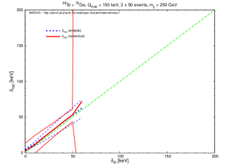
Without losing the generality, we assume that and set as . Note that the function should decrease monotonically as and/or increases. As sketched in Fig. A1, by, e.g. fixing and then checking whether by setting , , one should be able to find two auxiliary points and at which the function has a different sign ( corresponding to our current assumption). Now solve and , which satisfy and .
Since the intersection boundary of on the plane is almost a straight line and the analytic estimates should in principle be pretty close to the numerical solution , we approximate the equation of the boundary to a linear equation by
| (A22) |
namely,
| (A23) | |||||
Similarly, we define and asssum that . Here is the function of and given by Eq. (A18b). Then, by repeating the above process, one have
| (A24) | |||||
Finally, the numerical solution of can be given by
| (A25) |
Here we define
| (A26) | |||||
and
| (27a) | |||||
| (27b) | |||||
Here indicate the numerical estimates of the fitting parameters in the first round. One could process the whole numerical procedure iteratively. Remind however that statistical fluctuation could cause a divergency problem and the results from the later rounds might be worse than that from the first or second round.
Appendix C Expressions of the derivatives of , and
Firstly, differentiating the expression (34) for solving the characteristic energy with respect to , one find that
| (A28a) |
Then we can get
| (A29a) |
Similarly, differentiating the expression (34) with respect to , one has
Thus, it can be found that
| (A28b) |
Note that, as Eqs. (32) and (34), Eqs. (A29a) and (A28b) can be used for both of the analytically and numerically estimated and .
C.1 For the analytic estimates
C.2 For the numerical solutions
References
- [1] G. Jungman, M. Kamionkowski and K. Griest, “Supersymmetric Dark Matter”, Phys. Rep. 267, 195 (1996), arXiv:hep-ph/9506380.
- [2] G. Bertone, D. Hooper and J. Silk, “Particle Dark Matter: Evidence, Candidates and Constraints”, Phys. Rep. 405, 279 (2005), arXiv:hep-ph/0404175.
- [3] D. G. Cerdeo and A. M. Green, “Direct Detection of WIMPs”, contribution to “Particle Dark Matter: Observations, Models and Searches”, edited by G. Bertone, Cambridge University Press (2010), Chapter 17, Hardback ISBN 9780521763684, arXiv:1002.1912 [astro-ph.CO].
- [4] R. W. Schnee, “Introduction to Dark Matter Experiments”, arXiv:1101.5205 [astro-ph.CO] (2011).
- [5] W. Rau, “Dark Matter Search Experiments”, Phys. Part. Nucl. 42, 650 (2011), arXiv:1103.5267 [astro-ph.HE].
- [6] K. Freese, M. Lisanti and C. Savage, “Annual Modulation of Dark Matter: A Review”, Rev. Mod. Phys. 85, 1561–1581 (2013), arXiv:1209.3339 [astro-ph.CO].
- [7] DAMA Collab., R. Bernabei et al., “Search for WIMP Annual Modulation Signature: Results from DAMA/NaI-3 and DAMA/NaI-4 and the Global Combined Analysis”, Phys. Lett. B 480, 23 (2000); “First Results from DAMA/LIBRA and the Combined Results with DAMA/NaI”, Eur. Phys. J. C 56, 333 (2008), arXiv:0804.2741 [astro-ph]; “New Results from DAMA/LIBRA”, Eur. Phys. J. C 67, 39 (2010), arXiv:1002.1028 [astro-ph.GA].
- [8] DAMA Collab., R. Bernabei et al., “DAMA/LIBRA Results and Perspectives”, arXiv:1301.6243 [astro-ph.GA] (2013); “Dark Matter Investigation by DAMA at Gran Sasso”, Int. J. Mod. Phys. A 28, 1330022 (2013), arXiv:1306.1411 [astro-ph.GA].
- [9] CoGeNT Collab., C. E. Aalseth et al., “Results from a Search for Light–Mass Dark Matter with a P–Type Point Contact Germanium Detector”, Phys. Rev. Lett. 106, 131301 (2011), arXiv:1002.4703 [astro-ph.CO].
- [10] CoGeNT Collab., C. E. Aalseth et al., “Search for an Annual Modulation in a P–Type Point Contact Germanium Dark Matter Detector”, Phys. Rev. Lett. 107, 141301 (2011), arXiv:1106.0650 [astro-ph.CO].
- [11] J. Collar, “New Results from CoGeNT”, talk given at the IDM 2012 Workshop, Chicago, USA, July 23-27, 2012.
- [12] G. Angloher et al., “Results from 730 kg Days of the CRESST-II Dark Matter Search”, Eur. Phys. J. C 72, 1971 (2012), arXiv:1109.0702 [astro-ph.CO].
- [13] CDMS Collab., Z. Ahmed et al., “Results from the Final Exposure of the CDMS II Experiment”, Science 327, 1619 (2010), arXiv:0912.3592 [astro-ph.CO].
- [14] EDELWEISS Collab., E. Armengaud et al., “Final Results of the EDELWEISS-II WIMP Search Using a 4-kg Array of Cryogenic Germanium Detectors with Interleaved Electrodes”, Phys. Lett. B 702, 329 (2011), arXiv:1103.4070 [astro-ph.CO].
- [15] XENON100 Collab., E. Aprile et al., “Dark Matter Results from 100 Live Days of XENON100 Data”, Phys. Rev. Lett. 107, 131302 (2011), arXiv:1104.2549 [astro-ph.CO].
- [16] XENON100 Collab., E. Aprile et al., “Analysis of the XENON100 Dark Matter Search Data”, Astropart. Phys. 54, 11–24 (2014), arXiv:1207.3458 [astro-ph.IM] (2012); “Dark Matter Results from 225 Live Days of XENON100 Data”, Phys. Rev. Lett. 109, 181301 (2012), arXiv:1207.5988 [astro-ph.CO].
- [17] ZEPLIN-III Collab., D. Y. Akimov et al., “WIMP–Nucleon Cross–Section Results from the Second Science Run of ZEPLIN-III”, Phys. Lett. B 709, 14 (2012), arXiv:1110.4769 [astro-ph.CO].
- [18] KIMS Collab., S. C. Kim et al., “New Limits on Interactions between Weakly Interacting Massive Particles and Nucleons Obtained with CsI(Tl) Crystal Detectors”, Phys. Rev. Lett. 108, 181301 (2012), arXiv:1204.2646 [astro-ph.CO].
- [19] D. Tucker-Smith and N. Weiner, “Inelastic Dark Matter”, Phys. Rev. D 64, 043502 (2001), arXiv:hep-ph/0101138; “The Status of Inelastic Dark Matter”, Phys. Rev. D 72, 063509 (2005), arXiv:hep-ph/0402065.
- [20] S. Chang, G. D. Kribs, D. Tucker-Smith and N. Weiner, “Inelastic Dark Matter in Light of DAMA/LIBRA”, Phys. Rev. D 79, 043513 (2009), arXiv:0807.2250 [hep-ph].
- [21] J. March-Russell, C. McCabe and M. McCullough, “Inelastic Dark Matter, Non-Standard Halos and the DAMA/LIBRA Results”, J. High Energy Phys. 0905, 071 (2009), arXiv:0812.1931 [astro-ph].
- [22] K. Schmidt-Hoberg and M. W. Winkler, “Improved Constraints on Inelastic Dark Matter”, J. Cosmol. Astropart. Phys. 0909, 010 (2009), arXiv:0907.3940 [astro-ph.CO].
- [23] D. P. Finkbeiner, T. Lin and N. Weiner, “Inelastic Dark Matter and DAMA/LIBRA: An Experimentum Crucis”, Phys. Rev. D 80, 115008 (2009), arXiv:0906.0002 [astro-ph.CO].
-
[24]
D. B. Cline, W. Ooi and H. Wang,
“A Constrain on Inelastic Dark Matter Signal using ZEPLIN-II Results”,
arXiv:0906.4119 [astro-ph.CO] (2009);
ZEPLIN-III Collab., D. Y. Akimov et al., “Limits on Inelastic Dark Matter from ZEPLIN-III”, Phys. Lett. B 692, 180 (2010), arXiv:1003.5626 [hep-ex]. -
[25]
XENON10 Collab., J. Angle et al.,
“Constraints on Inelastic Dark Matter from XENON10”,
Phys. Rev. D 80, 115005 (2009),
arXiv:0910.3698 [astro-ph.CO] (2009);
XENON100 Collab., E. Aprile et al., “Implications on Inelastic Dark Matter from 100 Live Days of XENON100 Data”, Phys. Rev. D 84, 061101 (2011), arXiv:1104.3121 [astro-ph.CO]. - [26] S. Chang, R. F. Lang and N. Weiner, “Effect of Thallium Impurities in the DAMA Experiment on the Allowed Parameter Space for Inelastic Dark Matter”, Phys. Rev. Lett. 106, 011301 (2011), arXiv:1007.2688 [hep-ph].
- [27] CDMS Collab., Z. Ahmed et al., “Search for Inelastic Dark Matter with the CDMS II Experiment”, Phys. Rev. D 83, 112002 (2011), arXiv:1012.5078 [astro-ph.CO].
- [28] M. Drees and C.-L. Shan, “Reconstructing the Velocity Distribution of Weakly Interacting Massive Particles from Direct Dark Matter Detection Data”, J. Cosmol. Astropart. Phys. 0706, 011 (2007), arXiv:astro-ph/0703651.
- [29] M. Drees and C.-L. Shan, “Model–Independent Determination of the WIMP Mass from Direct Dark Matter Detection Data”, J. Cosmol. Astropart. Phys. 0806, 012 (2008), arXiv:0803.4477 [hep-ph].
- [30] C.-L. Shan, “Estimating the Spin–Independent WIMP–Nucleon Coupling from Direct Dark Matter Detection Data”, arXiv:1103.0481 [hep-ph] (2011); “Determining Ratios of WIMP–Nucleon Cross Sections from Direct Dark Matter Detection Data”, J. Cosmol. Astropart. Phys. 1107, 005 (2011), arXiv:1103.0482 [hep-ph].
- [31] DRIFT Collab., E. Daw et al., “Spin–Dependent Limits from the DRIFT-IId Directional Dark Matter Detector”, Astropart. Phys. 35, 397 (2012), arXiv:1010.3027 [astro-ph.CO]; “The DRIFT Dark Matter Experiments”, EAS Publ. Ser. 53, 11–18 (2012), arXiv:1110.0222 [physics.ins-det].
- [32] M. Felizardo et al., “Final Analysis and Results of the Phase II SIMPLE Dark Matter Search”, Phys. Rev. Lett. 108, 201302 (2012), arXiv:1106.3014 [astro-ph.CO].
- [33] D. Santos et al., “MIMAC: A Micro–Tpc Matrix Project for Directional Detection of Dark Matter”, EAS Publ. Ser. 53, 25–31 (2012), arXiv:1111.1566 [astro-ph.IM].
- [34] PICASSO Collab., S. Archambault et al., “Constraints on Low–Mass WIMP Interactions on from PICASSO”, Phys. Lett. B 711, 153 (2012), arXiv:1202.1240 [hep-ex].
- [35] COUPP Collab., E. Behnke et al., “First Dark Matter Search Results from a 4-kg CF3I Bubble Chamber Operated in a Deep Underground Site”, Phys. Rev. D 86, 052001 (2012), arXiv:1204.3094 [astro-ph.CO].
- [36] CDMS Collab., R. Agnese et al., “Silicon Detector Results from the First Five–Tower Run of CDMS II”, Phys. Rev. D 88, 031104 (2013), arXiv:1304.3706 [astro-ph.CO].
- [37] CDMS Collab., R. Agnese et al., “Dark Matter Search Results Using the Silicon Detectors of CDMS II”, Phys. Rev. Lett. 111, 251301 (2013), arXiv:1304.4279 [hep-ex] (2013).
- [38] LUX Collab., D. S. Akerib et al., “First Results from the LUX Dark Matter Experiment at the Sanford Underground Research Facility”, arXiv:1310.8214 [astro-ph.CO] (2013).
-
[39]
CDMS Collab., D. S. Akerib et al.,
“A Low–Threshold Analysis of CDMS Shallow–Site Data”,
Phys. Rev. D 82, 122004 (2010),
arXiv:1010.4290 [astro-ph.CO];
CDMS Collab., Z. Ahmed et al., “Results from a Low–Energy Analysis of the CDMS II Germanium Data”, Phys. Rev. Lett. 106, 131302 (2011), arXiv:1011.2482 [astro-ph.CO].