Inhomogeneous shear of orthotropic incompressible non-linearly elastic solids:
singular solutions
and biomechanical interpretation

Abstract

We present a detailed study of rectilinear shear deformation in the framework of orthotropic nonlinear elasticity, under Dirichlet and mixed-boundary conditions. We take a slab made of a soft matrix, reinforced with two families of extensible fibers. We consider the case where the shear occurs along the bissectrix of the angle between the two privileged directions aligned with the fibers. We show that if the two families of parallel fibers are mechanically equivalent, then only smooth solutions are possible, whereas if the mechanical differences among the two families of fibers is pronounced, then strain singularities may develop. We determine the precise conditions for the existence of such singular solutions for the standard reinforcing orthotropic model. We then extend our findings to some orthotropic models of interest in biomechanical applications, and we discuss the possible relevance of the singular solutions to biomechanics.

1 Introduction

Biological soft tissues exhibit complex mechanical behaviors, which are not easily accounted for by classic elastomeric constitutive models. The extension of the mathematical models of nonlinear elasticity from rubber to soft tissues continues to be a challenging area in theoretical biomechanics. For example, the presence of oriented collagen fiber bundles in blood vessels calls for the consideration of anisotropy in the mathematical modeling of the mechanics of arterial tissues, but the mathematical theory of nonlinear hyperelastic anisotropic materials is not as developed as the theory of isotropic nonlinear elasticity. A consultation of the eminent book by Antman [2] shows that, in recent years, there has been very few additions to the classical works of Adkins [3] or of Ericksen and Rivlin [4] with respect to the solution of boundary-value problems in nonlinear anisotropic elasticity.

It is well known that certain radial anisotropies in linear and non-linear elasticity problems can give rise to stress singularities which are absent in the corresponding isotropic version of these problems. Lekhnitskii [5] was perhaps the first to observe this peculiarity, by studying a circular orthotropic plate compressed by a uniformly distributed force along its external boundary. Antman and coworkers (see for example [6]) extended in some sense this analysis to radially symmetric equilibrium states of anisotropic nonlinearly elastic bodies. Another example of this extension to nonlinear elasticity is found in the paper by Kassianadis et al. [7] on the finite azimuthal shear of transversely isotropic materials.

Merodio et al. [8] investigated a simple model for a nonlinear, transversely isotropic, elastic solid and discovered a new kind of singular behavior, not present in isotropic materials. It occurs for the inhomogeneous rectilinear shear of an incompressible elastic slab reinforced by a family of parallel fibers. They show that, depending on the reinforcement strength and on the fiber orientation with respect to the shearing direction, weak solutions for this simple boundary value problem may be expected. These solutions are associated with fiber kinking and loss of ellipticity of the field equations. The deformation field is continuous, but it suffers a jump in the first derivative and a blow-up for the second derivative. Therefore the stress field suffers a discontinuity of first kind, a phenomenon clearly associated with mechanical instabilities. It also puts into question the applicability of finite element methods to nonlinear anisotropic elasticity, because the obtention of numerical solutions to the governing equations requires the calculation of second-, fourth-, and sometimes higher-order derivatives. In biomechanical applications of the constitutive models of arterial walls, the appearance of stress singularities is an important mathematical aspect of the theory, because it may be associated with some pathological states of the tissues (such as the bursting of an aneurysm).

The aim of the present paper is to extend the results of Merodio et al. [8] from transverse isotropy (one family of parallel fibers) to orthotropy (two families of parallel fibers), often encountered in biological soft tissues. We note that Fosdick and Royer-Carfagni [9] show that Lekhnitskii’s classical solution predicts the interpenetration of material regions, an unacceptable deformation behavior in the classical theory of elasticity. However the solutions proposed in [8] and here are isochoric and thus satisfy the local injectivity requirement.

The paper is organized as follows. In the next section we write down the governing equations and boundary conditions, and we discuss the basic mathematical issues at play. Section 3 is devoted to one of the simplest model of nonlinear orthotropic elastic materials (the standard reinforcing model), obtained by adding the classical neo-Hookean strain energy density to two terms that take into account the reinforcements along the fiber directions. These latter terms are quadratic in the squared extension along the fibers. We solve the problem of inhomogeneous rectilinear shear along the bissectrix to the fibers, first for Dirichlet boundary conditions and next for mixed boundary conditions. We also provide an energy analysis of the solutions. In Section 4 we consider a more advanced constitutive model of the biomechanics literature, proposed by Holzapfel et al [10], where the reinforcement terms in the strain-energy density are exponential, in order to account for a strong stiffening effect (the artery model).

The results suggest that orthotropic fiber reinforcement is quite efficient at cancelling the singularities and the shear discontinuities encountered in transversally isotropic fiber reinforcement. Indeed we recover the main features discovered by Merodio et al. [8] (jump in the shear, blow-up of the second derivative of the displacement) but under the condition that one family of fibers is much stiffer than the other. For the standard reinforcing model, one stiffness modulus must be at least 9.9 times larger than the other; for the artery model, the stiffnesses ratio is even higher, due to exponential terms. In general, the families of parallel collagen fibers found in arteries are determined experimentally to be mechanically equivalent, suggesting that singularities do not develop, at least in physiological conditions, for the rectilinear shear of arteries.

2 Basic equations

We consider a composite incompressible slab with thickness $L$, made of an isotropic matrix reinforced with two families of parallel extensible fibers (the fibers are all orthogonal to the boundaries of the solid.) In the undeformed configuration, we call $(X_{1},X_{2},X_{3})$ a set of Cartesian coordinates such that the solid is located in the $0\leqslant X_{3}\leqslant L$ region. We denote by $\boldsymbol{E}_{1}$, $\boldsymbol{E}_{2}$, $\boldsymbol{E}_{3}$ the orthogonal unit vectors defining the Lagrangian (reference) axes, aligned with the $X_{1}$, $X_{2}$, $X_{3}$ directions, respectively.

When the solid is sheared in the direction of $\boldsymbol{E}_{1}$, the particle initially at $\boldsymbol{X}$ moves to its current position $\boldsymbol{x}$. We call $\boldsymbol{F}=\partial\boldsymbol{x}/\partial\boldsymbol{X}$ the associated deformation gradient tensor, and $\boldsymbol{B}=\boldsymbol{F}^{t}\boldsymbol{F}$ the left Cauchy-Green strain tensor. We then call ($x_{1},x_{2},x_{3}$) the Cartesian coordinates, aligned with ($X_{1},X_{2},X_{3}$), corresponding to the current position $\boldsymbol{x}$. In the current configuration, the basis vectors are $\boldsymbol{e}_{1}$, $\boldsymbol{e}_{2}$, $\boldsymbol{e}_{3}$, and here they are such that $\boldsymbol{e}_{i}\equiv\boldsymbol{E}_{i}$ ($i=1,2,3)$. The deformation is given in all generality by

$$x_{1}=X_{1}+Lf(X_{3}/L),\qquad x_{2}=X_{2},\qquad x_{3}=X_{3},$$ (2.1)

where $f$ is a yet unknown function of $\eta\equiv X_{3}/L$ only. The amount of shear is $f^{\prime}=\text{d}f/\text{d}\eta$. The deformation (2.1) is a simple shear when $f^{\prime}$ is a constant; otherwise it is a rectilinear inhomogeneous shear. The direction of shear is that of $\boldsymbol{e}_{1}=\boldsymbol{E}_{1}$ and the plane of shear is that of $(\boldsymbol{e}_{1}=\boldsymbol{E}_{1},\boldsymbol{e}_{2}=\boldsymbol{E}_{2})$.

We find in turn that

$$\boldsymbol{F}=\boldsymbol{I}+f^{\prime}\boldsymbol{e}_{1}\otimes\boldsymbol{E}_{3},\qquad\boldsymbol{B}=\boldsymbol{I}+f^{\prime}(\boldsymbol{e}_{1}\otimes\boldsymbol{e}_{3}+\boldsymbol{e}_{1}\otimes\boldsymbol{e}_{3})+(f^{\prime})^{2}\boldsymbol{e}_{1}\otimes\boldsymbol{e}_{1}.$$ (2.2)

The first principal isotropic strain invariant $I_{1}\equiv\text{tr }\boldsymbol{B}$ is given here by

$$I_{1}=3+(f^{\prime})^{2},$$ (2.3)

and the second principal isotropic strain invariant, $I_{2}\equiv[I_{1}^{2}-\text{tr }(\boldsymbol{B}^{2})]/2$, is also equal to $3+(f^{\prime})^{2}$.

We call $\Phi$ ($\Psi$, respectively) the angle between the direction of one family of parallel fibers (the other family, respectively) and the direction of shear $X_{1}$. In other words, the unit vectors $\boldsymbol{M}$ and $\boldsymbol{N}$ (say) in the two preferred fiber directions have components

$$\boldsymbol{M}=\cos\Phi\boldsymbol{E}_{1}+\sin\Phi\boldsymbol{E}_{3},\qquad\boldsymbol{N}=\cos\Psi\boldsymbol{E}_{1}+\sin\Psi\boldsymbol{E}_{3},$$ (2.4)

and they are transformed into $\boldsymbol{m}=\boldsymbol{FM}$ and $\boldsymbol{n}=\boldsymbol{Fn}$ in the current configuration,

$$\boldsymbol{m}=(\cos\Phi+f^{\prime}\sin\Phi)\boldsymbol{e}_{1}+\sin\Phi\boldsymbol{e}_{3},\qquad\boldsymbol{n}=(\cos\Psi+f^{\prime}\sin\Psi)\boldsymbol{e}_{1}+\sin\Phi\boldsymbol{e}_{3}.$$ (2.5)

In the remainder of the paper, we restrict our attention to the special case where the material is sheared along a bisectrix of the angle between the two families. Generality is lost with this approach, but it has the merit of keeping low the number of geometric parameters; we also argue that it still captures some salient features of sheared soft tissues with two preferred directions.

Hence from now on, $\Psi=\pi-\Phi$ and the angle between the two preferred directions is $\pi-2\Phi$. In other words, the unit vectors $\boldsymbol{M}$ and $\boldsymbol{N}$ in the preferred fiber directions have components

$$\boldsymbol{M}=\cos\Phi\boldsymbol{E}_{1}+\sin\Phi\boldsymbol{E}_{3},\qquad\boldsymbol{N}=-\cos\Phi\boldsymbol{E}_{1}+\sin\Phi\boldsymbol{E}_{3},$$ (2.6)

in the reference configuration, and they are transformed into

$$\boldsymbol{m}=(\cos\Phi+f^{\prime}\sin\Phi)\boldsymbol{e}_{1}+\sin\Phi\boldsymbol{e}_{3},\qquad\boldsymbol{n}=(-\cos\Phi+f^{\prime}\sin\Phi)\boldsymbol{e}_{1}+\sin\Phi\boldsymbol{e}_{3},$$ (2.7)

in the current configuration; Figure 1 is a visualization of the situation in the case of a simple (homogeneous) shear of amount $0.5$ and an angle $\Phi=60^{\circ}$. Note that because the reinforcements are not directional, we may without loss of generality restrict ourselves to the range $0<\Phi<\pi$.

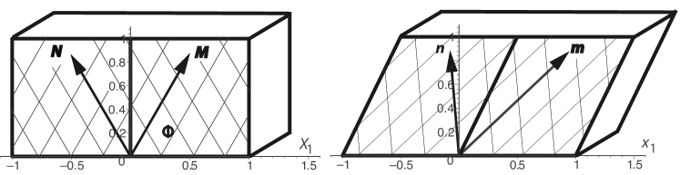
Figure 1: Two unit squares lying in the transverse section of a slab reinforced with two families of fibers (thin lines) and subject to a simple shear of amount $0.5$ along the bissectrix of the angle between the two families. In the reference configuration, one family of fibers is aligned with the unit vector $\boldsymbol{M}$ making an angle $\Phi=60^{\circ}$ with the $X_{1}$-axis; the other family is aligned with $\boldsymbol{N}$, at an angle $120^{\circ}$ with the $X_{1}$-axis. In the current configuration, they are along $\boldsymbol{m}$ and $\boldsymbol{n}$, respectively.

We now introduce the anisotropic invariants $I_{4}\equiv\boldsymbol{m\cdot m}$ and $I_{5}\equiv\boldsymbol{Fm\cdot}\boldsymbol{Fm}$; in particular we find

$$I_{4}=1+f^{\prime}\sin 2\Phi+(f^{\prime})^{2}\sin^{2}\Phi.$$ (2.8)

Recall that $I_{4}$ is the squared stretch in the fiber direction (Spencer [11]). In particular, if $I_{4}\geqslant 1$ then the fibers aligned with $\boldsymbol{m}$ are in extension, and if $I_{4}\leqslant 1$ then they are in compression. Clearly here, when $0\leqslant\Phi\leqslant\pi/2$, the quantity $I_{4}-1$ is always positive and the fibers aligned with $\boldsymbol{m}$ are in extension. On the other hand, when $\pi/2<\Phi<\pi$, there always exist a certain amount of shear (explicitly, $-2/\tan\Phi$) above which these fibers are in compression.

The other anisotropic invariants are $I_{6}\equiv\boldsymbol{n\cdot n}$, $I_{7}\equiv\boldsymbol{Fn\cdot}\boldsymbol{Fn}$, and $I_{8}\equiv\boldsymbol{m\cdot n}$. Here we find that

$$I_{6}=1-f^{\prime}\sin 2\Phi+(f^{\prime})^{2}\sin^{2}\Phi.$$ (2.9)

In general, the strain-energy density $W$ of a hyperelastic incompressible solid reinforced with one or two families of parallel extensible fibers depends on two isotropic deformation invariants: $I_{1}$ and $I_{2}$, and on the five anisotropic deformation invariants [11, 12]: $I_{4}$, …, $I_{8}$. Henceforth we make the assumption that $W$ is the sum of an isotropic part and an anisotropic part. For the isotropic part, modelling the properties of the elastin matrix, we take the neo-Hookean strain-energy density, with constant shear modulus $\mu$. For the anisotropic part, modelling the properties of the extensible collagen fibers, we take the sum of a function of $I_{4}$ only and a function of $I_{6}$ only, say $F(I_{4})+G(I_{6})$. Hence we restrict our attention to those solids with strain energy density

$$W=\mu(I_{1}-3)/2+F(I_{4})+G(I_{6}).$$ (2.10)

Now the Cauchy stress tensor $\boldsymbol{\sigma}$ derived from this strain energy function is (see e.g. Ogden, 1984),

$$\boldsymbol{\sigma}=-p\boldsymbol{I}+\mu\boldsymbol{B}+2F^{\prime}(I_{4})\boldsymbol{m}\otimes\boldsymbol{m}+2G^{\prime}(I_{6})\boldsymbol{n}\otimes\boldsymbol{n},$$ (2.11)

where $p$ is a Lagrange multiplier introduced by the constraint of incompressibility, and $F^{\prime}\equiv\text{d}F/\text{d}I_{4}$, $G^{\prime}\equiv\text{d}G/\text{d}I_{4}$.

Because shear is a plane strain deformation, and because the fibers lie in the plane of shear, it is a simple matter to find the directions of principal stresses. One is normal to the plane of shear, and the two others are in the ($\boldsymbol{e}_{1},\boldsymbol{e}_{3}$) plane, at the angles $\varphi$ and $\varphi+\pi/2$ from the direction of shear, where $\varphi\in]0,\pi/4]$ is defined by

$$\tan 2\varphi=2(\boldsymbol{e}_{1}\cdot\boldsymbol{\sigma e}_{3})/(\boldsymbol{e}_{1}\cdot\boldsymbol{\sigma e}_{1}-\boldsymbol{e}_{3}\cdot\boldsymbol{\sigma e}_{3}).$$ (2.12)

Here we find that

$$\boldsymbol{e}_{1}\cdot\boldsymbol{\sigma e}_{3}=\mu f^{\prime}+2F^{\prime}(I_{4})m_{1}m_{3}+2G^{\prime}(I_{6})n_{1}n_{3},$$ (2.13)

where $m_{i}\equiv\boldsymbol{m\cdot e}_{i}$ and $n_{i}\equiv\boldsymbol{n\cdot e}_{i}$ are found from (2.7).

The equilibrium equations, $\text{div }\boldsymbol{\sigma}=\boldsymbol{0}$ (in the abscence of body forces) reduce to

$$\dfrac{\partial p}{\partial x_{1}}=\dfrac{\text{d}}{\text{d}x_{3}}\left[\mu f^{\prime}+2F^{\prime}(I_{4})m_{1}m_{3}+2G^{\prime}(I_{6})n_{1}n_{3}\right],$$ (2.14)

$$\dfrac{\partial p}{\partial x_{2}}=0,$$

$$\dfrac{\partial p}{\partial x_{3}}=\dfrac{\text{d}}{\text{d}x_{3}}\left[\mu f^{\prime}+2F^{\prime}(I_{4})m_{3}^{2}+2G^{\prime}(I_{6})n_{3}^{2}\right],$$

where the expressions in brackets are independent of $x_{1}$ and $x_{2}$. It follows that

$$p=p(x_{1},x_{2})=C_{0}x_{1}+2F^{\prime}(I_{4})m_{3}^{2}+2G^{\prime}(I_{6})n_{3}^{2}+D,$$ (2.15)

where $C_{0}$, $D$ are arbitrary constants of integration, is a suitable pressure field. A single governing equation remains to be solved for the shear deformation, namely

$$\dfrac{\text{d}}{\text{d}\eta}\left[\mu f^{\prime}+2F^{\prime}(I_{4})m_{1}m_{3}+2G^{\prime}(I_{6})n_{1}n_{3}\right]=C_{0}L.$$ (2.16)

We consider two specific boundary value problems (BVPs). In the reference configuration, the slab of thickness $L$ in the $X_{3}$ direction and of infinite dimensions in the other directions is bonded to two infinite rigid plates located at $X_{3}=0$ and $X_{3}=L$. A constant pressure gradient is applied in the $x_{1}$ direction and drives the deformation of the slab. The overall goal of our investigation is to solve (2.16) subject (i) to the Dirichlet boundary conditions: $f(0)=0,\,f(1)=0$, and (ii) to the mixed boundary conditions: $f(0)=0,\,f^{\prime}(1)=K_{1}$, where $K_{1}$ is a prescribed constant. In Case (i), we have a classical two-point boundary value problem which, for an isotropic medium, may be reduced to a Cauchy problem by using symmetry considerations. In our anisotropic case it may happen that, once the second-order differential equation (2.16) is rewritten in normal form, the corresponding right handside is neither continuous nor Lipschitzian with respect to $f^{\prime}$. Then standard methods for the study of the existence and uniqueness of the solution may not apply any longer; moreover, the solution may develop singularities. In Case (ii), the BVP is simpler to solve, but it is also possible to have non-smooth solutions. We point out that enforcing the boundary condition $f^{\prime}(1)=K_{1}$ is equivalent to prescribing the shear stress $T_{12}$ on the upper face of the slab.

For transversally isotropic materials, Case (i) has been studied by Merodio et al [8] and a mixed-BVP similar to Case (ii) has been considered for azimuthal shear by Kassianadis et al [7].

3 The standard reinforcing model

3.1 Normal form of the BVP

The standard reinforcing model for solids with two family of fibers is a special case of (2.10). Its strain energy density is

$$W=\mu(I_{1}-3)/2+\mu E_{1}(I_{4}-1)^{2}/4+\mu E_{2}(I_{6}-1)^{2}/4,$$ (3.1)

where $\mu E_{1}$ and $\mu E_{2}$ are the extensional moduli in the fiber directions. The BVPs based on (2.16) are now

$$\dfrac{\text{d}}{\text{d}\eta}\left[f^{\prime}+E_{1}(I_{4}-1)m_{1}m_{3}+E_{2}(I_{6}-1)n_{1}n_{3}\right]=C_{0}L/\mu;$$ (3.2)

with the boundary conditions (i): $f(0)=0,\,f(1)=1$ and (ii): $f(0)=0,\,f^{\prime}(1)=K_{1}$. We begin our study with the Dirichlet boundary conditions, Case (i).

The differential equation may be rewritten as

$$\dfrac{\text{d}}{\text{d}\eta}\left\{f^{\prime}+\gamma f^{\prime}\sin^{2}\Phi[2\cos^{2}\Phi+3\beta(f^{\prime})\sin\Phi\cos\Phi+(f^{\prime})^{2}\sin^{2}\phi]\right\}=C_{0}L/\mu,$$ (3.3)

where we introduced the dimensionless material constants $\gamma$ and $\beta$, defined as

$$\gamma=E_{1}+E_{2},\qquad\beta=(E_{1}-E_{2})/(E_{1}+E_{2}).$$ (3.4)

The quantity $\gamma$ gives a measure of the collagen/elastin strength ratio, and the quantity $\beta$ gives a measure of the orthotropy. If $\gamma=0$, then the material is isotropic. If $\beta=\pm 1$, then either $E_{1}=0$ or $E_{2}=0$ and the solid is transversally isotropic (there is only one active family of parallel fibers); if $\beta=0$, then $E_{1}=E_{2}$ and the two families of fibers are said to be mechanically equivalent.

In its normal form, the BVP Case (i) reads

$$\dfrac{\text{d}^{2}f}{\text{d}\eta^{2}}=\dfrac{\alpha}{D(f^{\prime},\Phi)},\qquad f(0)=f(1)=0,$$ (3.5)

where $\alpha\equiv C_{0}L/\mu$ is a dimensionless measure of the pressure gradient and where the denominator $D$ is defined as

$$D(f^{\prime},\Phi)=1+\gamma\sin^{2}\Phi[2\cos^{2}\Phi+6\beta\cos\Phi\sin\Phi(f^{\prime})+3\sin^{2}\Phi(f^{\prime})^{2}].$$ (3.6)

First we note that when $\beta=1$, the whole analysis is consistent with that of Merodio et al. [8] for a transversally isotropic slab. Also, when $\beta=0$, the governing equation coincides with that obtained for the rectilinear inhomogeneous shear of the isotropic solid slab with strain energy density $W=(\mu+2\gamma\sin^{2}\Phi\cos^{2}\Phi)(I_{1}-3)/2+(\gamma\sin^{4}\Phi)(I_{1}-3)^{2}/4$. It follows that when the two families of fibers are mechanically equivalent, only smooth solutions exist and no singularity may develop.

Next we take $\beta\neq 0$ and notice that $D$ is a quadratic in the amount of shear $f^{\prime}$. If its discriminant is negative, then no singularity may develop. The denominator $D$ has real roots when

$$\left(3\beta^{2}-2\right)\gamma\sin^{2}{2\Phi}-4\geq 0.$$ (3.7)

Therefore a necessary condition for the appearance of singularities is that

$$\beta^{2}>2/3.$$ (3.8)

Assume that the fibers along $\boldsymbol{M}$ are stiffer than those along $\boldsymbol{N}$. Then $E_{1}>E_{2}$ and this inequality means that $E_{1}/E_{2}>5+2\sqrt{6}\simeq 9.9$. Hence we are certain that singularities do not develop when the fibers along $\boldsymbol{M}$ are less than $9.9$ times stiffer than the fibers along $\boldsymbol{N}$.

3.2 Orthogonal fibers: $\Phi=\pi/4$

Here we focus on the special case where one family of fibers is orthogonal to the other family ($\Phi=\pi/4$). Then the denominator $D$ in (3.6) reduces to

$$D(f^{\prime},\pi/4)=1+(\gamma/4)\left[2+6\beta(f^{\prime})+3(f^{\prime})^{2}\right].$$ (3.9)

Clearly, whether $f^{\prime\prime}$ develops singularities or not depends among other things on the sign of the quantity $(3\beta^{2}-2)\gamma-4$. Figure 2 displays on the left the curve where this quantity is zero in the ($\beta,\gamma$) plane. When it is negative, the existence and uniqueness of a smooth solution are guaranteed by general theorems and standard numerical procedures of integration can be implemented. For instance, we take $\beta=0.5$, $\gamma=3.0$, and $\alpha=1.0,5.0,10.0$ in turn, and obtain the displacements displayed on the right of Figure 2, using the finite difference method implemented into Maple.

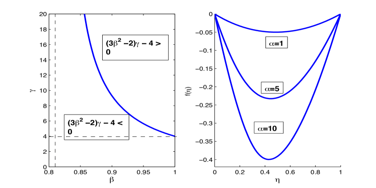
Figure 2: On the left: curve in the ($\beta,\gamma$) plane separating the region where only smooth exist ($(3\beta^{2}-2)\gamma-4<0$) from the region where singularities might develop for the second derivative of the displacement, in the case where the two families of fibers are orthogonal. On the right: an example of a completely smooth solution, obtained for $\beta=0.5$, $\gamma=3.0$ and for several values of the pressure gradient, as measured by $\alpha$.

When $(3\beta^{2}-2)\gamma-4\geqslant 0$, there is a chance that singularities may develop within the thickness of the slab and we now investigate this possibility. First we consider the case where this discriminant is equal to zero, when $\gamma=4/(3\beta^{2}-2)$. Then

$$D=\dfrac{3}{3\beta^{2}-2}(f^{\prime}+\beta)^{2},$$ (3.10)

and integrating (3.5) once gives

$$(f^{\prime}+\beta)^{3}=\alpha(3\beta^{2}-2)(\eta-\eta_{0})+\beta^{3},$$ (3.11)

where $\eta_{0}\in(0,1)$ is a point in the thickness of the slab where $f^{\prime}=0$ (its existence is ensured by the continuity and differentiability of $f$, coupled to the boundary conditions $f(0)=f(1)=0$). Solving for $f^{\prime}$ gives

$$f^{\prime}(\eta)=\mp\left[\beta^{3}+\alpha(3\beta^{2}-2)(\eta-\eta_{0})\right]^{1/3}-\beta,$$ (3.12)

where the sign depends on the sign of the radical. Integrating further, and imposing $f(0)=0$, we obtain

$$f(\eta)=\dfrac{3}{4\alpha(3\beta^{2}-2)}\left\{\left[\beta^{3}+\alpha(3\beta^{2}-2)(\eta-\eta_{0})\right]^{4/3}\right.\\ \left.-\left[\beta^{3}-\alpha(3\beta^{2}-2)\eta_{0}\right]^{4/3}\right\}-\beta\eta.$$ (3.13)

To solve the BVP entirely, it remains to determine $\eta_{0}\in(0,1)$. It is fixed by the second boundary condition: $f(1)=0$, i.e. it is a solution to the equation

$$\left[\beta^{3}+\alpha(3\beta^{2}-2)(1-\eta_{0})\right]^{4/3}-\left[\beta^{3}-\alpha(3\beta^{2}-2)\eta_{0}\right]^{4/3}=4\alpha\beta(3\beta^{2}-2)/3.$$ (3.14)

Now, collecting (3.5), (3.10), (3.11), we see that $f^{\prime\prime}$ blows up at $\eta=\eta_{S}$ given by

$$\alpha(3\beta^{2}-2)(\eta_{S}-\eta_{0})+\beta^{3}=0.$$ (3.15)

The final condition to impose for this singularity is that it occurs within the thickness of the slab: $0\leqslant\eta_{S}\leqslant 1$, i.e.

$$0\leqslant\eta_{0}-\dfrac{\beta^{3}}{\alpha(3\beta^{2}-2)}\leqslant 1.$$ (3.16)

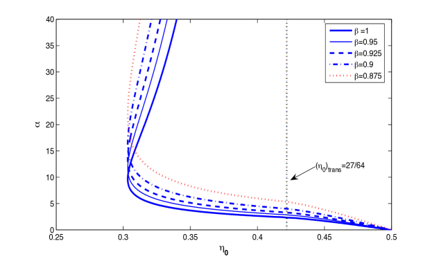
Figure 3: Curves in the ($\eta_{0},\alpha$) plane giving the locus of the constant of integration $\eta_{0}$ corresponding to a given level of pressure gradient, as measured by $\alpha$, in the case where the two families of fibers are orthogonal and some fibers are stiff enough to guarantee the appearance of singularities. The curves are shown in the first quarter of the plane, for $\beta=0.875,0.9,0.925,0.95,1.0$. They are antisymmetric with respect to the point $(0.5,0)$ (second part not shown here). The curves are limited to the right by a vertical line at $\eta_{0}=27/64=0.421875$.

On Figure 3 we graph the curves defining the pairs ($\eta_{0},\alpha$) such that the second boundary condition (3.14) is satisfied, for several values of $\beta$. We limit the display to the range $\eta_{0}<0.5$ because the curves are antisymmetric with respect to the point $(0.5,0)$. For visual reasons, the upper bound is taken as $\alpha_{\text{max}}=40.0$. The other limit of each curve is imposed by the inequalities (3.16), specifically here the lower one. The corresponding transitional behavior is dictated by the equality

$$\eta_{0}=(\eta_{0})_{\text{trans}}\equiv\dfrac{\beta^{3}}{\alpha(3\beta^{2}-2)}.$$ (3.17)

When this holds, the corresponding transitional level of pressure gradient is found from (3.14) as

$$\alpha=(\alpha)_{\text{trans}}\equiv\dfrac{64\beta^{3}}{27(3\beta^{2}-2)}.$$ (3.18)

Substituting back above gives

$$(\eta_{0})_{\text{trans}}=27/64=0.421875.$$ (3.19)

Hence all the curves stop at the vertical barrier $\eta_{0}=0.421875$, irrespective of the value of $\beta$.

For all values of $\alpha$ and $\eta_{0}$ such that the point ($\alpha,\eta_{0}$) belongs to one of these curves, a singularity develops within the thickness for the second derivative of the displacement. For instance at the points ( $(\alpha)_{\text{trans}},(\eta_{0})_{\text{trans}}$), the exact solution (3.13) and its derivatives reduce to

$$f(\eta)=\beta\left(\eta^{4/3}-\eta\right),\quad f^{\prime}(\eta)=\beta\left[(4/3)\eta^{1/3}/3-1\right],\quad f^{\prime\prime}(\eta)=(4/9)\beta\eta^{-2/3},$$ (3.20)

and $f^{\prime\prime}$ clearly blows up on the $\eta=0$ face of the slab. For Figure 4 we take $\beta=0.875$ and three points on the corresponding curve of Figure 3 , namely ($\alpha=5.3489,\eta_{0}=(\eta_{0})_{\text{trans}}$), ($\alpha=10.0,\eta_{0}=0.33120$), and ($\alpha=15.0,\eta_{0}=0.30871$). For the first combination, $f^{\prime\prime}$ blows up on the slab face $\eta=0$; for the second and third combinations, it blows up within the thickness of the slab.

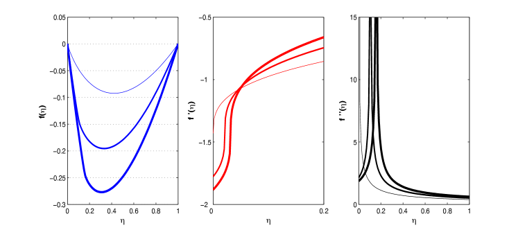
Figure 4: Plots of the displacement and of its first and second derivatives through the slab thickness in the case where the two families of fibers are orthogonal and singularities develop. Here $\beta=0.875$ (large difference in fiber stiffness) and $\alpha$ (giving a measure of the pressure gradient) and $\eta_{0}$ (constant of integration) are chosen so that the second derivative is discontinuous. Thin curves: $\alpha=5.3489$, $\eta_{0}=0.421875$); Medium thickness curves: $\alpha=10.0$, $\eta_{0}=0.33120$; Thick curves: $\alpha=15.0$, $\eta_{0}=0.30871$.

Next we consider the case where the discriminant of the $f^{\prime}$ quadratic in (3.9) is positive: $(3\beta^{2}-2)\gamma-4>0$, and focus now on finding singularities for $f^{\prime}$, the amount of shear. Integrate the BVP (3.5), (3.9) once to get

$$g(f^{\prime})=\alpha(\eta-\eta_{0}),$$ (3.21)

where $\eta_{0}$ is a constant of integration, and $g$ is the following cubic,

$$g(x):=\left(1+\dfrac{\gamma}{2}\right)x+\dfrac{3\beta\gamma}{4}x^{2}+\dfrac{\gamma}{4}x^{3},$$ (3.22)

with a local maximum (resp. minimum) at $x_{1}$ (resp. $x_{2}$) defined as

$$x_{1,2}=-1\mp\sqrt{\dfrac{(3\beta^{2}-2)\gamma-4}{3\gamma}}.$$ (3.23)

For $g_{1}\equiv g(x_{1})$ and $g_{2}\equiv g(x_{2})$, we find

$$g_{1,2}=-\dfrac{1}{6}\left[2(2+\beta)+\gamma(1-\beta)(3\beta-2)\right]\pm\dfrac{\gamma}{2}\left[\dfrac{(3\beta^{2}-2)\gamma-4}{3\gamma}\right]^{3/2}.$$ (3.24)

Clearly, a systematic procedure to establish a one-to-one correspondence between $x$ and $g$ everywhere (or equivalently, between $f^{\prime}$ and $\eta$) runs into difficulties in the interval $x_{1}\leqslant x\leqslant x_{3}$, where $x_{3}$ is the root of $g(x)=g_{1}$ other than $x_{1}$, see Figure 5(a).

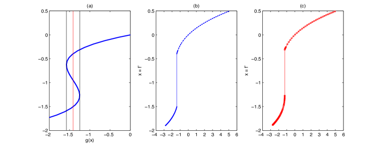
Figure 5: (a) Plot of the cubic establishing a relationship between the amount of shear and the thickness. When $g_{1}\leqslant\eta\leqslant g_{2}$, there are three possible values of $f^{\prime}$ for each $\eta$. The vertical dashed lines are at $\eta=g_{1},g_{2}$; the vertical full line defines two regions of equal area between $g_{1}$ and $g_{2}$. (b) Maxell rule convention: jump in the amount of shear at the thickness giving equal areas. (c) Maximum delay convention: jump in the amount of shear at $\eta=g_{1}$. Here the Dirichlet BVP is solved for $\beta=0.95$, $\gamma=10.0$, $\alpha=10.0$.

To address this problem, we take the stance that $f^{\prime}$ jumps from a low value to a higher one. In order to jump following the absolute minima of the energy, we consider in turn the Maxwell rule convention of equal area, see Figure 5(b), and the Maximum delay convention, see Figure 5(c). We propose to track these two possible solutions by a suitable numerical approach. This hands-on approach is required because usual numerical methods sometimes fail in finding good approximations. In fact, commercial code solvers issue a warning here about possible failure in the numerical convergence and are unable to provide a satisfactory solution in this region. Note that the non-monotonous behavior does not necessarily occur within the slab thickness and that some parameter values allow a monotonous variation of $f^{\prime}$, devoid of jumps (such is for instance the case when $g_{1}\geqslant 1$). We focus on those parameter values which do give a jump inside the slab.

The main difficulty in solving the Dirichlet BVP is that we do not have an analytical access to the value of the integration constant $\eta_{0}$ in (3.21). We tackle the Dirichlet BVP by a shooting method, combined with the bisection method, in the following manner.

We take $\eta_{0}^{(0)}$ (say) as an initial guess for $\eta_{0}$. Then let $K_{0}^{(0)}\equiv f^{\prime}(0)$; it is the real root to the cubic $g(K_{0}^{(0)})=-\alpha\eta_{0}^{(0)}$. It is now possible to reformulate the BVP as an Initial Value Problem (IVP), which we solve numerically on two subintervals of $[0,1]$. That process is detailled later, in the simpler case of the mixed BVP. It gives $\eta_{S}^{(0)}$, the thickness where the jump takes place, and also $f(\eta)$ numerically. Finally we compute $f(1)$ and measure how different it is from the second boundary condition $f(1)=0$: if $|f(1)|\leqslant\;$tol is not satisfied, for a prescribed numerical tolerance “tol”, then we adjust the approximate value of $\eta_{0}$ from $\eta_{0}^{(0)}$ to $\eta_{0}^{(1)}$ and so on, from $\eta_{0}^{(k-1)}$ to $\eta_{0}^{(k)}$, until the criterion of convergence is reached, following the indications given by the bissection method. In the process we also get access to $\eta_{S}^{(k)}$, a numerical approximation of the singularity point $\eta_{S}$.

In Figure 6, we report the numerical solutions for $\gamma=10.0$, $\alpha=10.0$, and in turn, $\beta=1.0$ and $\beta=0.95$, with tol=$1e$-6 as the tolerance for the stopping criterium in the bissection method. The values identified by the bisection method for the integration constants are as follows. When $\beta=1.0$ (transverse isotropy), we find $\eta_{0}=0.2423$ for the Maxwell rule solution and $\eta_{0}=0.21725$ for the Maximum delay solution; when $\beta=0.95$ (orthotropy), we find $\eta_{0}=0.13818$ for the Maxwell rule solution and $\eta_{0}=0.05014$ for the Maximum delay solution. It is worth noting that the two kinds of solutions not only jump at different singular points, but also present different slopes, before and after the singular points. Moreover, we checked that the solutions obtained for $\beta=1.0$ (transverse isotropy) are consistent with those obtained by Merodio et al. [8], using a different numerical method, based on a quadrature approach.

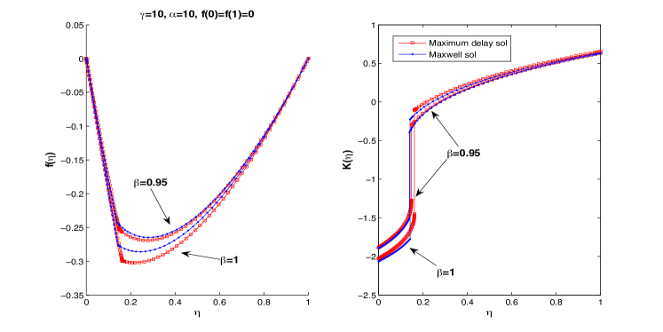
Figure 6: Maxwell rule solutions and Maximum delay solutions for $\beta=1.0$ (transverse isotropy) and for $\beta=0.95$ (orthotropy), with zero Dirichlet boundary conditions. Here $\gamma=10.0$, $\alpha=10.0$.

We now consider the mixed BVP, Case (ii),

$$\dfrac{\text{d}^{2}f}{\text{d}\eta^{2}}=\dfrac{\alpha}{D(f^{\prime},\Phi)},\qquad f(0)=0,\qquad f^{\prime}(1)=K_{1},$$ (3.25)

which turns out to be simpler to analyze and to solve numerically than the Dirichlet BVP.

The main features uncovered in the previous analysis still apply. Hence the uniqueness of the solution is not guaranteed for all parameter values, because the energy can have two minima and is in general not a convex function, leading to a jump in the derivative of the displacement. The analysis for the mixed boundary conditions is almost identical to that of the Dirichlet boundary conditions, with the difference that it is now possible to identify a priori the location of the singularity.

In order to jump following the absolute minima of the energy, again we consider in turn the Maxwell rule convention of equal area, and the Maximum delay convention, because commercial solvers also fail here. We track these solutions by transforming the mixed BVP into a second-order initial value problem (IVP), as follows.

Starting from the first integral (3.21)-(3.22) of equation (3.3), we find from the second boundary condition $f^{\prime}(1)=K_{1}$ that

$$\eta_{0}=1-g(K_{1})/\alpha.$$ (3.26)

Then let $K_{0}\equiv f^{\prime}(0)$; it is the real root to the cubic

$$g(K_{0})=-\alpha\eta_{0}=g(K_{1})-\alpha.$$ (3.27)

Now we can reformulate the BVP as an IVP, which we solve numerically in two steps. First on the subinterval $[0,\eta_{S}]$, with initial conditions: $f(0)=0$, $f^{\prime}(0)=K_{0}$; we call $f_{S}$ and $K_{S}$ the computed values of $f$ and $f^{\prime}$ at $\eta=\eta_{S}$, the slab thickness where the jump takes place. Next we solve numerically the second part of the IVP, this time on the subinterval $[\eta_{S},1]$, with initial values: $f(\eta_{S})=f_{S}$, $f^{\prime}(\eta_{S})=K_{S}$. To compute the value of $\eta_{S}$, the singularity thickness, we proceed as follows.

In the case of the Maxwell rule convention of equal area, the singularity occurs at the inflection point of the function $g$. Solving $g^{\prime\prime}(K_{S})=0$ gives $K_{S}=-\beta$ and then, $g(K_{S})=\beta[\gamma(\beta^{2}-1)/2-1]$. Then $\eta_{S}$ is found by solving the equation

$$g(K_{S})=g(K_{1})+\alpha(\eta_{S}-1).$$ (3.28)

In the case of the Maximum delay convention, the singularity occurs at the local maximum of the function $g$. Hence $K_{S}=x_{1}$ given by (3.23); then $g(K_{S})=g_{1}$ given by (3.24), and $\eta_{S}$ is found from (3.28) for $\eta_{S}$.

Figure 7 shows the numerical solutions obtained with this numerical technique for the values $\gamma=10.0$, $\alpha=10.0$, $K_{1}=0.5$, and in turn, $\beta=1.0$ (transverse isotropy) and $\beta=0.95$ (orthotropy). In the figure on the left, we report the numerical approximation for $f(\eta)$ and in the figure on the right, the approximations for the amount of shear $f^{\prime}(\eta)$, clearly showing that the jumps of the derivatives occur at different singular points. For that example, we find $\eta_{0}=0.48125$ when $\beta=1.0$ and $\eta_{0}=0.44375$ when $\beta=0.95$.

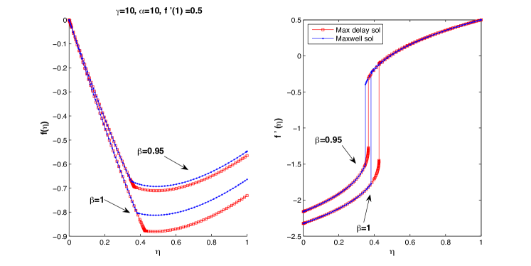
Figure 7: Plots of the displacement and of its first derivative through the slab thickness in the case where the two families of fibers are orthogonal. Numerical solutions for the mixed BVP obtained by following the Maxwell rule convention (round dots plots) and the Maximum delay convention (square dots plots), for $\beta=1.0$ (transverse isotropy) and $\beta=0.95$ (orthotropy), and $\gamma=10.0$, $\alpha=10.0$, $K_{1}=f^{\prime}(1)=0.5$.

3.3 Non-orthogonal fibers: $\Phi\neq\pi/4$

Extending the results and techniques developed at $\Phi=\pi/4$ to the case $\Phi\neq\pi/4$ (non-orthogonal fibers) poses no particular problem. Rather than detailing the process, we refer the reader to the paper by Merodio et al., [8] where the extension is done in the case $\beta=1$ (transverse isotropy).

4 Orthotropic biomechanical model

We now investigate briefly whether the analysis conducted for the standard reinforcing model can be extended to a strain energy density often encountered in the biomechanics literature, namely the model proposed by Holzapfel et al. [10] to describe the behavior of an orthotropic artery, and widely used since, for instance to model porcine aortic tissue, passive basilar artery, cornea, etc. We present it in the form

$$W=\dfrac{\mu}{2}(I_{1}-3)+\dfrac{\mu E_{1}}{2k_{1}}\left\{\exp\left[k_{1}(I_{4}-1)^{2}\right]-1\right\}\\ +\dfrac{\mu E_{2}}{2k_{2}}\left\{\exp\left[k_{2}(I_{6}-1)^{2}\right]-1\right\},$$ (4.1)

where $k_{1}$, $k_{2}$ are dimensionless constants. Equation (2.16) is then rewritten as

$$\frac{d}{d\eta}\left\{f^{\prime}+E_{1}(I_{4}-1)\exp\left[k_{1}(I_{4}-1)^{2}\right]m_{1}m_{3}\right.\\ \left.+E_{2}(I_{6}-1)\exp\left[k_{2}(I_{6}-1)^{2}\right]n_{1}n_{3}\right\}=C_{0}L/\mu.$$ (4.2)

The BVP can be put in the form (3.5), where now

$$D(f^{\prime},\Phi)=1+\sin\Phi\left\{E_{1}\Gamma_{1}(f^{\prime},\Phi)\exp\left[k_{1}(I_{4}-1)^{2}\right]\right.\\ \left.+E_{2}\Gamma_{2}(f^{\prime},\Phi)\exp\left[k_{2}(I_{6}-1)^{2}\right]\right\},$$ (4.3)

and the functions $\Gamma_{1}$ and $\Gamma_{2}$ are defined as

$$\Gamma_{1}=2k_{1}f^{\prime 2}\left(f^{\prime}\sin\Phi+\cos\Phi\right)\left(f^{\prime}\sin^{2}\Phi+\sin 2\Phi\right)^{2}\left(2f^{\prime}\sin^{2}\Phi+\sin 2\Phi\right)\\ +3(f^{\prime})^{2}\sin^{3}\Phi+3f^{\prime}\sin\Phi\sin 2\Phi+\cos\Phi\sin 2\Phi,$$ (4.4)

and

$$\Gamma_{2}=2k_{2}f^{\prime 2}\left(f^{\prime}\sin\Phi-\cos\Phi\right)\left(f^{\prime}\sin^{2}\Phi-\sin 2\Phi\right)^{2}\left(2f^{\prime}\sin^{2}\Phi-\sin 2\Phi\right)\\ -3(f^{\prime})^{2}\sin^{3}\Phi+3f^{\prime}\sin\Phi\sin 2\Phi+\cos\Phi\sin 2\Phi.$$ (4.5)

To simplify the algebra we restrict our discussion to the special case where the families of fibers are at right angle, $\Phi=\pi/4$. Our objective is to find out if there exist special values $f^{\prime}=(f^{\prime})^{*}$ say, such that $D((f^{\prime})^{*},\pi/4)=0$. Now $\Gamma_{1}$ and $\Gamma_{2}$ reduce to

$$\Gamma_{1}(f^{\prime},\pi/4)=\frac{\sqrt{2}}{4}\left\{f^{\prime 2}(f^{\prime}+1)^{2}(f^{\prime}+2)^{2}k_{1}+(3f^{\prime 2}+6f^{\prime}+2)\right\},$$

$$\Gamma_{2}(f^{\prime},\pi/4)=\frac{\sqrt{2}}{4}\left\{f^{\prime 2}(f^{\prime}-1)^{2}(f^{\prime}-2)^{2}k_{2}+(3f^{\prime 2}-6f^{\prime}+2)\right\}.$$ (4.6)

In the biomechanical applications of the model (4.1), it is often assumed that the two families of fibers are mechanically equivalent, so that $E_{1}=E_{2}$ and $k_{1}=k_{2}$. In that case, some long but simple computations show that $f^{\prime}\equiv 0$ is a minimum for the function $D$. Because $D(0,\pi/4)=1+E_{1}\neq 0$, we conclude that singularities may not develop (This result may be extended to any angle $\Phi$ quite easily).

When $E_{1}\neq E_{2}$, things are more complex. For instance, consider the values of $D(f^{\prime},\pi/4)$ when $f^{\prime}=-1,0,1$ in turn:

$$D(-1,\pi/4)=1-E_{1}\textrm{e}^{k_{1}/4}+(36k_{2}+11)(E_{2}/4)\textrm{e}^{3k_{2}/2},$$

$$D(0,\pi/4)=1+(E_{1}+E_{2})/2,$$

$$D(1,\pi/4)=1+(36k_{1}+11)(E_{1}/4)\textrm{e}^{3k_{2}/2}-E_{2}\textrm{e}^{k_{2}/4}.$$ (4.7)

Therefore, because $D(0,\pi/4)>0$, it is sufficient to choose

$$\exp(k_{1}/4)E_{1}>1+\frac{36k_{2}+11}{4}\exp(9k_{2}/4)E_{2}$$ (4.8)

to obtain the existence of at least one $(f^{\prime})^{*}$ such that $D((f^{\prime})^{*},\pi/4)=0$. This inequality suggests that singularities occur only for huge differences between the fiber stiffnesses, and are unlikely to be observed at all for realistic values of the parameters. Take for example the case where $k_{1}=k_{2}=k$ (say). Then $\beta$ defined in (3.4) gives a measure of the orthotropy: when $\beta=1$, the solid is reinforced with one family of parallel fibers, and when $\beta<1$, there are two families of parallel fibers at play. To generate the graphs in Figure 8, we take $k=0.1$ and $\beta=1.0$, $0.9$, $0.875$, and $0.82$ in turn. At $\beta=1.0$, the shear variations are pronounced but regular. As soon as $\beta<1$ (two families of fibers), the shear variations are quickly smoothed down, highlighting the stabilizing effect of orthotropy.

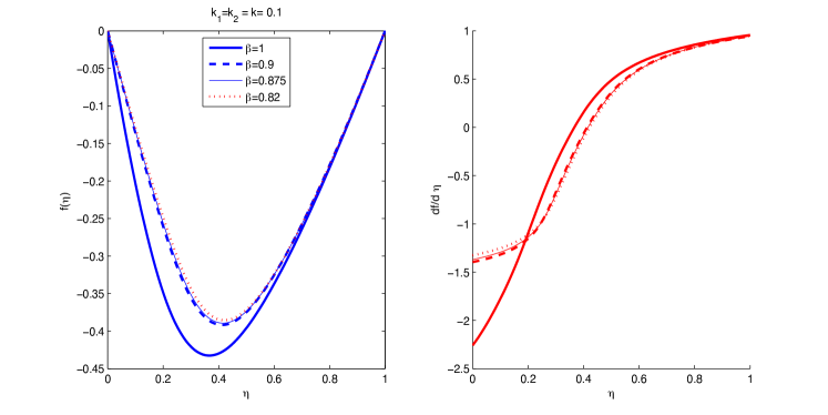
Figure 8: Numerical solution to the zero Dirichlet BVP for the aartery model. Here $k_{1}=k_{2}=0.1$ and $\beta=1.0$ (transverse isotropy), $0.9$, $0.875$, $0.82$ (orthotropy). Other parameters: $E_{1}+E_{2}=10.0$, $C_{0}L/\mu=10.0$.

We now evoke some possible applications of our results to biomechanics. Indeed, we know that arterial tissue adapts to physiological and pathological stimuli though rearrangement of the microstructure. Arterial remodeling is induced by chronically altered mechanical forces; if for some pathological reason, the remodeling of the fibers introduces some disparity in the various directions in the stiffness of the fibers, then it may happen that $E_{1}\neq E_{2}$ and that some “dangerous” mechanical behavior develops. However, from a mathematical point of view the solutions of the BVPs suggest that the artery model is much more stable than the standard reinforcing model, due to the presence of exponential terms in the determining equations.

5 Concluding remarks

We extended the results of Merodio et al. [8] from transverse isotropy to orthotropy. The most important finding is that orthotropic materials may develop singular solutions only if there is a significant difference between the mechanical stiffnesses of the two families of fibers. We quantified this result rigorously for the standard reinforcing model, where a necessary condition for the formation of singular solutions is that $\beta^{2}>2/3$, which means that one family of fibers must be at least 9.9 times stiffer than the other family.

When we consider the arterial strain-energy density (4.1), analytical results are no longer possible, but the methodology used to study the standard reinforcing material is still applicable. In this case a huge difference between $E_{1}$ and $E_{2}$ is necessary to possibly introduce a singularity. However, if the fibers are mechanically equivalent, as is usual for biological soft tissues, then singular solutions are avoided altogether. Therefore biological networks, such as the collageneous structure of arterial walls, are the right structure to prevent the formation of the singularities described here.

From a theoretical point of view, our results demonstrate the complexity of finite anisotropic elasticity and deliver some exact solutions, which are scarce in the literature on finite inhomogeneous deformations of orthotropic materials.

It is important to note that we have barely scratched the surface of the collection of problems associated with the rectilinear shear of solids reinforced by two families of parallel fibers. Primo, we relied on strong —and perhaps, reductive— constitutive assumptions, namely that the strain energy density can be split into the sum of an isotropic part and an anisotropic part, and that this latter part is also the sum of two parts, each depending on only one anisotropic invariant. Although there is now a good body of experimental data supporting the adequacy of the standard reinforcing model (3.1) and of the biomechanics arterial model (4.1), the importance or insignificance of other constitutive arguments must also be evaluated, such as the role played by other invariants [13] or by the angular distribution of fiber directions [14, 15, 16]. Secondo, we limited our study to a shear occurring along the bissectrix of the two families of parallel fibers, and did not study the influence of other orientations. Intuitively, it is expected that this is the direction where the coupled reinforcing effect of the fibers is at its strongest. Nevertheless we were able to show that if one family of fibers is much stiffer than the other for the standard reinforcing model, then singularities might develop in the thickness of the clamped slab, in the form of discontinuities in the shear or in the strain gradient.

References

- [1]
- [2] S.S. Antman, Nonlinear Problems of Elasticity, Springer Verlag, New York, 1995.
- [3] J.E. Adkins, Proc. Roy. Soc. London A 231 (1955) 75-90.
- [4] J.L. Ericksen, R.S. Rivlin, J. Rational Mech. Analysis 3 (1954) 281-301.
- [5] S.G. Lekhnitskii, Anisotropic Plates, Gordon & Breach, New York (1968).
- [6] S.S. Antman, P.V. Negron Marrero, J. Elasticity 18 (1987) 131-164.
- [7] F. Kassianidis, J. Merodio, R.W. Ogden, T.J. Pence, Math. Mech. Solids (to appear).
- [8] J. Merodio, G. Saccomandi, I. Sgura, Int. J. Non-Linear Mech. 42 (2007) 342-354.
- [9] R. Fosdick, G. Royer-Carfagnig, Proc. Roy. Soc. London A 457 (2001) 2167-2187.
- [10] G.A. Holzapfel, T.C. Gasser, R.W. Ogden, J. Elasticity 61 (2000), 1-48.
- [11] A.J.M. Spencer, Deformations of fiber-Reinforced Materials. University Press, Oxford (1972).
- [12] J.P. Boehler, Applications of tensor functions in solid mechanics, in: CISM Lecture Notes 292, Springer Verlag, New York (1987).
- [13] J. Merodio, R.W. Ogden, Int. J. Non-Linear Mech. 41 (2006) 556-563.
- [14] A.S. Milani, J.A. Nemes, R.C. Abeyaratne, G.A. Holzapfel, Composites A: Appl. Sc. Manufact. 38 (2007) 1493-1501.
- [15] T.C. Gasser, R.W. Ogden, G.A. Holzapfel, Roy. Soc. Interface 3 (2006) 15-35.
- [16] A. Pandolfi, G.A. Holzapfel, J. Biomech. Eng. (in press).
- [17]