Abstract

We present an approach to decomposition and factor analysis of matrices with ordinal data. The matrix entries are grades to which objects represented by rows satisfy attributes represented by columns, e.g. grades to which an image is red, a product has a given feature, or a person performs well in a test. We assume that the grades form a bounded scale equipped with certain aggregation operators and conforms to the structure of a complete residuated lattice. We present a greedy approximation algorithm for the problem of decomposition of such matrix in a product of two matrices with grades under the restriction that the number of factors be small. Our algorithm is based on a geometric insight provided by a theorem identifying particular rectangular-shaped submatrices as optimal factors for the decompositions. These factors correspond to formal concepts of the input data and allow an easy interpretation of the decomposition. We present illustrative examples and experimental evaluation.

Keywords: factor analysis, ordinal data, fuzzy relation, fuzzy logic, concept lattice

1 Introduction

Problem Description

Data dimensionality reduction is fundamental for understanding and management of data. In traditional approaches, such as factor analysis, a decomposition of an object-variable matrix is sought into an object-factor matrix and a factor-variable matrix with the number of factors reasonably small. Compared to the original variables, the factors are considered more fundamental concepts, which are hidden in the data. Their discovery and interpretation, which is central importance in our paper, helps better understand the data.

In this paper, we consider decompositions of matrices $I$ with a particular type of ordinal data. Namely, each entry $I_{ij}$ of $I$ represents a grade to which the object corresponding to the $i$th row has, or is incident with, the attribute corresponding to the $j$th row. Examples of such data are results of questionnaires where respondents (rows) rate services, products, etc., according to various criteria (columns); results of performance evaluation of people (rows) by various tests (columns); or binary data in which case there are only two grades, $0$ (no, failure) and $1$ (yes, success). Our goal is to decompose an $n\times m$ object-attribute matrix $I$ into a product

$$I=A\circ B$$ (1)

of an $n\times k$ object-factor matrix $A$ and a $k\times m$ factor-attribute matrix $B$ with the number $k$ of factors as small as possible.

The scenario is thus similar to ordinary matrix decomposition problems but there are important differences. First, we assume that the entries of $I$, i.e. the grades, as well as the entries of $A$ and $B$ are taken from a bounded scale $L$ of grades, such as the real unit interval $L=[0,1]$ or the Likert scale $L=\{1,\dots,5\}$ of degrees of satisfaction. Second, the matrix composition operation $\circ$ used in our decompositions is not the usual matrix product. Instead, we use the t-norm-based product with a t-norm $\otimes$ being a function used for aggregation of grades. In particular, $A\circ B$ is defined by

$$(A\circ B)_{ij}=\textstyle\bigvee_{l=1}^{k}A_{il}\otimes B_{lj}.$$ (2)

where $\bigvee$ denoted the supremum (maximum, if $L$ is linearly ordered). The ordinary Boolean matrix product is a particular case of this product in which the scale $L$ has $0$ and $1$ as the only grades and $a\otimes b=\min(a,b)$. Also, when $A$ and $B$ are thought of as fuzzy relations, $A\circ B$ is exactly the usual composition of fuzzy relations, see e.g. [12, 14]. It is to be emphasized that we attempt to treat graded incidence data in a way which is compatible with its semantics. This need has been recognized long ago in mathematical psychology, in particular in measurement theory [16]. For example, even if we represent the grades by numbers such as $0\sim\,$strongly disagree, $\frac{1}{4}\sim\,$disagree, …, $1\sim\,$strongly agree, addition, multiplication by real numbers, and linear combination of graded incidence data may not have natural meaning. Consequently, decomposition of a matrix $I$ with grades into the ordinary matrix product of arbitrary real-valued matrices $A$ and $B$ suffers from a difficulty to interpret $A$ and $B$, as well as to interpret the way $I$ is reconstructed from, or explained by, $A$ and $B$. This is not to say that the usual matrix decompositions of incidence data $I$ may not be useful. For example, [20, 29] report that decompositions of binary matrices into real-valued matrices may yield better reconstruction accuracies. Hence, as far as the dimensionality reduction aspect (the technical aspect) is concerned, ordinary decompositions may be favorable. However, when the knowledge discovery aspect plays a role, attention needs to be paid to the semantics of decomposition. Our algorithm is based on [5], in particular on using formal concepts of $I$ as factors. This is important both from the technical viewpoint, since due to [5] optimal decompositions may be obtained this way, and the knowledge discovery viewpoint, since formal concepts may naturally be interpreted.

Related Work

Recently, new methods of matrix decomposition and dimensionality reduction have been developed. One aim is to have methods which are capable of discovering possibly non-linear relationships between the original space and the lower dimensional space [24, 30]. Another is driven by the need to take into account constraints imposed by the semantics of the data. Examples include nonnegative matrix factorization, in which the matrices are constrained to those with nonnegative entries and which leads to additive parts-based discovery of features in data [17]. Another example, relevant to this paper, is Boolean matrix decomposition. Early work on this problem was done in [23, 27] which already include complexity results showing the hardness of problems related to Boolean matrix decompositions. Recent work on this topic includes [6, 9, 19, 20, 23]. As was mentioned above, Boolean matrix decomposition is a particular case of the problem considered in this paper. In particular, the present approach is inspired by [6].

Note also that partly related to this paper are methods for decomposition of binary matrices into non-binary ones such as [18, 25, 26, 28, 34], see also [29] for further references.

2 Decomposition and Factors

2.1 Decomposition and the Factor Model

As was mentioned above, we assume that for the problem of finding a decomposition (1) of $I$ with the matrix product defined by (2), the set $L$ of grades forms a bounded scale equipped with an aggregation operation $\otimes$. In particular, we assume that $L$ is a complete lattice bounded by $0$ and $1$ and that $\otimes$ is a binary operation on $L$ that is commutative, associative, has $1$ as its neutral element, and commutes with suprema, i.e.

$$\textstyle a\otimes\bigvee_{k\in K}b_{k}=\bigvee_{k\in K}(a\otimes b_{k}).$$

Note that this in particular implies $a\otimes 1=a$. It is well-known, see e.g. [12, 13, 15], that for any such operation, one may define its residuum $\to$ by

$$a\rightarrow b=\max\{c\in L\,|\,a\otimes c\leq b\}.$$

The residuum satisfies an important technical condition called adjointness, namely,

$$a\otimes b\leq c\mbox{ if{}f }a\leq b\rightarrow c.$$

$L$ together with $\otimes$ and $\rightarrow$ satisfying the above conditions forms a complete residuated lattice [32].

Complete residuated lattices are well known in fuzzy logic where are used as the structures of truth degrees with $\otimes$ and $\to$ being the truth functions of (many-valued) conjunction and implication. Important examples include those with $L=[0,1]$ and $\otimes$ being a continuous t-norm, such as $a\otimes b=\min(a,b)$ (Gödel t-norm), $a\otimes b=a\cdot b$ (Goguen t-norm), and $a\otimes b=\max(0,a+b-1)$ (Łukasiewicz t-norm); or $L$ being a finite chain equipped with the restriction of Gödel t-norm, Łukasiewicz t-norm, or other suitable operation. Since these matters are routinely known, we omit details and refer the reader for further examples and properties of residuated lattices to [12, 13, 15].

Consider now the meaning of the factor model given by (1) and (2). The matrices $A$ and $B$ represent relationships between objects and factors, and between factors and the original attributes. We interpret $A_{il}$ as the degree to which the factor $l$ applies to the object $i$, i.e. the truth degree of the proposition “factor $l$ applies to object $i$”; and $B_{lj}$ as the degree to which the attribute $j$ is a particular manifestation of the factor $l$, i.e. the truth degree of the proposition “attribute $j$ is a manifestation of factor $l$”. Therefore, due to basic principles of fuzzy logic, if $I=A\circ B$, the discovered factors explain the original relationship between objects and attributes, represented by $I$, via $A$ and $B$ as follows: the degree $I_{ij}$ to which the object $i$ has the attribute $j$ equals the degree of the proposition “there exists factor $l$ such that $l$ applies to $i$ and $j$ is a particular manifestation of $l$”.

As the nature of the relationship between objects and attributes via factors is traditionally of interest, it is worth noting that in our case, the attributes are expressed by means of factors in a non-linear manner:

Example 1.

With Łukasiewicz t-norm, let $I=A\circ B$ be

$$\left(\begin{array}[]{ccc}0.3&0.0&0.1\\ 0.3&0.7&0.5\\ 0.5&0.8&0.6\end{array}\right)=\left(\begin{array}[]{cc}0.2&0.8\\ 0.9&0.8\\ 1.0&1.0\end{array}\right)\circ\left(\begin{array}[]{ccc}0.4&0.8&0.6\\ 0.5&0.2&0.3\end{array}\right)\!\!.$$

Then for $Q_{1}=(0.6\ 0.2)$ and $Q_{2}=(0.4\ 0.3)$ we have $(Q_{1}+Q_{2})\circ B=(1.0\ 0.5)\circ B=(0.4\ 0.8\ 0.6)\not=(0.0\ 0.6\ 0.2)=(0.0\ 0.4\ 0.2)+(0.0\ 0.2\ 0.0)=Q_{1}\circ B+Q_{2}\circ B$.

2.2 Factors for Decomposition

We now need to recall a result from [5] saying that optimal decompositions of $I$ may be attained by using formal concepts of $I$ as factors. Denote by $L^{U}$ the set of all fuzzy sets in a set $U$ with truth degrees from $L$, i.e. the set of all mappings from $U$ to $L$, and put $X=\{1,\dots,n\}$ (objects) and $Y=\{1,\dots,m\}$ (attributes).

A formal concept of $I$ is any pair $\langle C,D\rangle$ of fuzzy sets $C\in L^{X}$ and $D\in L^{Y}$ for which $C^{\uparrow}=D$ and $D^{\downarrow}=C$ where the operators ${}^{\uparrow}\!:L^{X}\rightarrow L^{Y}$ and ${}^{\downarrow}\!:L^{Y}\rightarrow L^{X}$ are defined by

$$C^{\uparrow}(j) =\textstyle\bigwedge_{i\in X}(C(i)\rightarrow I_{ij})\quad\text{and}\quad D^{\downarrow}(i)=\textstyle\bigwedge_{j\in Y}(D(j)\rightarrow I_{ij}).$$

Here, $\bigwedge$ is the infimum in $L$ (in our case, since $X$ and $Y$ are finite, infimum coincides with minimum if $L$ is linearly ordered). The set

$${\cal B}(X,Y,I)=\{\langle C,D\rangle\in L^{X}\times L^{Y}\mid C^{\uparrow}=D\mbox{ and }D^{\downarrow}=C\}$$

of all formal concepts of $I$ is called the concept lattice of $I$ and forms indeed a complete lattice when equipped with a natural subconcept-superconcept ordering, see [4] for details. Formal concepts are simple models of concepts in the sense of traditional, Port-Royal logic. For a formal concept $\langle C,D\rangle$, $C$ and $D$ are called the extent and the intent of $\langle C,D\rangle$; the degrees $C(i)$ and $D(j)$ are interpreted as the degrees to which the concept applies to object $i$ and attribute $j$, respectively. The graded setting takes into account that most concepts used by humans are graded rather than clear-cut.

For a set ${\cal F}=\{\langle C_{1},D_{1}\rangle,\dots,\langle C_{k},D_{k}\rangle\}$ of formal concepts of $I$ with a fixed order given by the indices, denote by $A_{\cal F}$ and $B_{\cal F}$ the $n\times k$ and $k\times m$ matrices defined by

$$(A_{\cal F})_{il}=(C_{l})(i)\quad\mbox{and}\quad(B_{\cal F})_{lj}=(D_{l})(j).$$

That is, the $l$th column of $A_{\cal F}$ consists of grades assigned to the objects by $C_{l}$ and the $l$th row of $B_{\cal F}$ consists of grades assigned to attributes by $D_{l}$.

If $I=A_{\cal F}\circ B_{\cal F}$, $\cal F$ can be seen as a set of factors which fully explain the data. In such a case, we call the formal concepts from $\cal F$ factor concepts. In this case, the factors have a natural, easy-to-understand meaning as is demonstrated in Section 4. Let $\rho(I)$ denote the Schein rank of $I$, i.e.

$$\rho(I)=\min\{k\mid I=A\circ B\mbox{ for some }n\times k\mbox{ and }k\times m\mbox{ matrices }A\mbox{ and }B\}.$$

The following theorem was proven in [5].

Theorem 1.

For every $n\times m$ matrix $I$ with entries from $L$ there exists a set ${\cal F}\subseteq{\cal B}(X,Y,I)$ containing exactly $\rho(I)$ formal concepts for which $I=A_{\cal F}\circ B_{\cal F}.$

The theorem says that, in a sense, formal concepts of $I$ are optimal factors for decompositions. It follows that when looking for decompositions of $I$, one can restrict the search to the set of formal concepts instead of the set of all possible decompositions.

3 Algorithm and Complexity of Decompositions

To prevent misunderstanding, let us define our problem precisely. For a given (that is, constant for the problem) structure of truth degrees, i.e. set $L$ equipped with the lattice operations and $\otimes$ and $\to$, the problem we discuss is a minimization (optimization) problem [2] specified as follows:

Input:	$n\times m$ matrix $I$ with entries from $L$;
Feasible Solution:	$n\times k$ and $k\times m$ matrices $A$ and $B$ with entries
	from $L$ for which $I=A\circ B$;
Cost of Solution:	$k$.

As indicated above, due to Theorem 1, we look for feasible solutions $A$ and $B$ in the form $A_{\mathcal{F}}$ and $B_{\mathcal{F}}$ for some $\mathcal{F}$. Therefore, the algorithm we present in Section 3.1 computes a set $\mathcal{F}$ of formal concepts of $I$ for which $A_{\mathcal{F}}$ and $B_{\mathcal{F}}$ is a good feasible solution. Our algorithm runs in polynomial time but produces only suboptimal solutions, i.e. $|\mathcal{F}|\geq\rho(I)$. As is shown in Section 3.2, this is a consequence of a fundamental limitation. Namely, unless P=NP, there does not exist a polynomial time algorithm producing optimal solutions to the decomposition problem. We demonstrate experimentally in Section 4, however, that the quality of the solutions provided by our algorithm is reasonable.

In this section as well as in Section 4 we need the following “geometric” insight. Let us note that every formal concept $\langle C_{l},D_{l}\rangle\in\mathcal{F}$ induces a matrix $J_{l}=C_{l}\otimes D_{l}$ given by

$$(C_{l}\otimes D_{l})_{ij}=C_{l}(i)\otimes D_{l}(j),$$ (3)

the rectangular matrix induced by $\langle C_{l},D_{l}\rangle$ (it results by the Cartesian product of $C_{l}$ and $D_{l}$). Then $I=A_{\cal F}\circ B_{\cal F}$ means that

$$I_{ij}=(J_{1})_{ij}\vee\cdots\vee(J_{k})_{ij},$$ (4)

i.e. $I$ is the $\bigvee$-superposition of $J_{l}$s.

3.1 Algorithm

Throughout this section, we assume that $L$ is linearly ordered, i.e. $a\leq b$ or $b\leq a$ for any two degrees $a,b\in L$. (The general, non-linear case can be handled with no substantial difficulty but we prefer to keep things simple, particularly because of the practical importance of the linear case.) In such case, (4) implies that $I=A_{\cal F}\circ B_{\cal F}$ if and only if for each $\langle i,j\rangle\in\{1,\dots,n\}\times\{1,\dots,m\}$ there exists $\langle C_{l},D_{l}\rangle\in\mathcal{F}$ for which

$$I_{ij}=C_{l}(i)\otimes D_{l}(j).$$ (5)

In case of (5), we say that $\langle C_{l},D_{l}\rangle$ covers $\langle i,j\rangle$. This allows us to see that the problem of finding a set $\mathcal{F}$ of formal concepts of $I$ for which $I=A_{\cal F}\circ B_{\cal F}$ can be reformulated as the problem of finding $\mathcal{F}$ such that every pair from the set

$$\mathcal{U}=\{\langle i,j\rangle\,|\,I_{ij}\neq 0\}$$ (6)

is covered by some $\langle C_{l},D_{l}\rangle\in\mathcal{F}$. Since $C_{l}(i)\otimes D_{l}(j)\leq I_{ij}$ is always the case [3], we need not worry about overcovering. We now see that every instance of our decomposition problem may be rephrased as an instance of the well-known set cover problem, see e.g. [2, 7] in which the set to be covered is $\mathcal{U}$ and the system of sets that may be used to cover $\mathcal{U}$ is

$$\{\{\langle i,j\rangle\,;\,I_{ij}\leq C(i)\otimes D(j)\}\mid\langle C,D\rangle\in\mathcal{B}(X,Y,I)\}.$$

Accordingly, one can use the well-known greedy approximation algorithm [2] for solving set cover to select a set $\mathcal{F}$ for formal concepts for which $I=A_{\cal F}\circ B_{\cal F}$. However, this would be a costly way from the computational complexity point of view. Namely, one would need to compute the possibly rather large set $\mathcal{B}(X,Y,I)$ first and, worse, repeatedly iterate over this set in the greedy set cover algorithm.

Instead, we propose a different greedy algorithm. The idea is to supply promising candidate factor concepts on demand during the factorization procedure, as opposed to computing all candidate factor concepts beforehand. The algorithm generates the promising candidate factor concepts by looking for promising columns. A technical property which we utilize is the fact that for each formal concept $\langle C,D\rangle$,

$$D=\textstyle\bigcup_{j\in Y}\{{}^{D(j)\!}/j\}^{\downarrow\uparrow},$$

i.e. each intent $D$ is a union of intents $\{{}^{D(j)\!}/j\}^{\downarrow\uparrow}$ [4] and that $C=D^{\downarrow}$ by definition. Here, $\{{}^{D(j)\!}/j\}$ denotes a graded singleton, i.e.

$$\{{}^{D(j)\!}/j\}(j^{\prime})=\left\{\begin{array}[]{ll}D(j)&\text{if }j^{\prime}=j,\\ 0&\text{if }j^{\prime}\not=j.\end{array}\right.$$

As a consequence, we may construct any formal concept by adding sequentially $\{{}^{a\!}/j\}^{\downarrow\uparrow}$ to the empty set of attributes. Our algorithm follows a greedy approach that makes us select $j\in Y$ and a degree $a\in L$ which maximize the size of

$$D\oplus_{a}j=\{\langle k,l\rangle\!\in\mathcal{U}\,|\,D^{+\downarrow}(k)\otimes D^{+\downarrow\uparrow}(l)\geq I_{kl}\},$$ (7)

where $D^{+}=D\cup\{{}^{a\!}/j\}$ and $\cal U$ denotes the set of $\langle i,j\rangle$ of $I$ (row $i$, column $j$) for which the corresponding entry $I_{ij}$ is not covered yet. At the start, $\mathcal{U}$ is initialized according to (6). As the algorithm proceeds, $\mathcal{U}$ gets updated by removing from it the pairs $\langle i,j\rangle$ which have been covered by the selected formal concept $\langle C,D\rangle$. Note that $|D\oplus_{a}j|$ is the number of entries of $I$ which are covered by formal concept $\langle D^{+\downarrow},D^{+\downarrow\uparrow}\rangle$, i.e. by the concept generated by $D^{+}$, the intent of the current candidate concept $\langle C,D\rangle$ extended by $\{{}^{a\!}/j\}$. Therefore, instead of going through all possible formal concepts and selecting the factors from them, we just go through columns and degrees and add them repeatedly as to maximize the value $V$ of the corresponding formal concepts, until such addition is possible. The resulting algorithm is summarized below.

Find-Factors$(I)$
1	$\ignorespaces\mathcal{U}\leftarrow\{\langle i,j\rangle\,|\,I_{ij}\neq 0\}$
2	$\ignorespaces\mathcal{F}\leftarrow\emptyset$
3	$\ignorespaces\mbox{\bf while\ }\mathcal{U}\neq\emptyset$
4	do $D\leftarrow\emptyset$
5	$\ignorespaces V\leftarrow 0$
6	$\ignorespaces\!\!\mbox{ {select} }\langle j,a\rangle\mbox{ {that maximizes} }|D\oplus_{a}j|$
7	$\ignorespaces\mbox{\bf while\ }|D\oplus_{a}j|>V$
8	do $V\leftarrow|D\oplus_{a}j|$
9	$\ignorespaces D\leftarrow(D\cup\{{}^{a\!}/j\})^{\downarrow\uparrow}$
10	$\ignorespaces\!\!\mbox{ {select} }\langle j,a\rangle\mbox{ {that maximizes} }|D\oplus_{a}j|$
11	$\ignorespaces C\leftarrow D^{\downarrow}$
12	$\ignorespaces\mathcal{F}\leftarrow\mathcal{F}\cup\{\langle C,D\rangle\}$
13	$\ignorespaces\mbox{\bf for\ }\langle i,j\rangle\in\mathcal{U}$
14	do if $I_{ij}\leq C(i)\otimes D(j)$
15	then
16	$\ignorespaces\mathcal{U}\leftarrow\mathcal{U}\mathop{\backslash}\{\langle i,j\rangle\}$
17	$\ignorespaces\mbox{\bf return\ }\mathcal{F}$

The main loop of the algorithm (lines 3–16) is executed until all the nonzero entries of $I$ are covered by at least one factor in $\mathcal{F}$. The code between lines 4 and 10 constructs an intent by adding the most promising columns. After such an intent $D$ is found, we construct the corresponding factor concept and add it to $\mathcal{F}$. The loop between lines 13 and 16 ensures that all matrix entries covered by the last factor are removed from $\mathcal{U}$. Obviously, the algorithm is sound and finishes after finitely many steps (polynomial in terms of $n$ and $m$) with a set $\mathcal{F}$ of factor concepts.

3.2 Complexity of Finding Optimal Decompositions

As mentioned above, there is no guarantee that our algorithm finds an optimal decomposition, i.e. the one with $k=\rho(I)$. The following theorem shows that, unless P=NP, no polynomial time algorithm which finds optimal decompositions exists.

Theorem 2.

The decomposition problem, i.e. the problem to find for a given $n\times m$ matrix $I$ with grades an $n\times k$ matrix $A$ and a $k\times m$ matrix $B$ for which $I=A\circ B$ with $k$ as small as possible, is NP-hard.

Proof.

The theorem is an easy consequence of established reductions, see [22, 23] and also [6, 20, 31]. Namely, by definition of NP-hardness of optimization problems, we need to show that the corresponding decision problem is NP-complete. The decision problem, which we denote by $\Pi$ in what follows, is to decide for a given $I$ and positive integer $k$ whether there exists a decomposition $I=A\circ B$ with the inner dimension $k$ or smaller. Now, $\Pi$ is NP-complete because the decision version of the set basis problem, which is known to be NP-complete [27], is reducible to it. The decision version of the set basis problem is: Given a collection $S=\{S_{1},\dots,S_{n}\}$ of sets $S_{i}\subseteq\{1,\dots,m\}$ and a positive integer $k$, is there a collection $P=\{P_{1},\dots,P_{k}\}$ of subsets $P_{l}\subseteq\{1,\dots,m\}$ such that for every $S_{i}$ there is a subset $Q_{i}\subseteq\{P_{1},\dots,P_{k}\}$ for which $\bigcup Q_{i}=S_{i}$ (i.e., the union of all sets from $Q_{i}$ is equal to $S_{i}$)? This problem is easily reducible to $\Pi$: Given $S$, define an $n\times m$ matrix $I$ by $I_{ij}=1$ if $j\in S_{i}$ and $I_{ij}=0$ if $j\not\in S_{i}$. Such reduction works for every $L$ and $\otimes$ because we always have $1\otimes 1=1$ and $1\otimes 0=0\otimes 1=0\otimes 0=0$. Namely, one can check that if $I=A\circ B$ for $n\times k$ and $k\times m$ matrices $A$ and $B$ with entries from $L$ then $P_{l}$ ($l=1,\dots,k$) and $Q_{i}$, defined by $j\in P_{l}$ if $B_{lj}=1$ and $P_{l}\in Q_{i}$ if $A_{il}=1$, represent a solution to the set basis problem given by $S$. Conversely, if $P_{l}$ and $Q_{l}$ represent a solution to the set basis problem, the matrices $A$ and $B$ defined by $B_{lj}=1$ if $j\in P_{l}$ and $B_{lj}=0$ if $j\not\in P_{l}$, and $A_{il}=1$ if $P_{l}\in Q_{i}$ and $A_{il}=0$ if $P_{l}\not\in Q_{i}$, are matrices with entries from $L$ which represent a solution to $\Pi$. ∎

4 Examples and Experiments

In Section 4.1, we examine in detail a factor analysis of 2004 Olympic Decathlon data. We include this example to illustrate the notions involved in our methods but most importantly to argue that the algorithm developed in this paper can be used to obtain reasonable factors from data with grades. In Section 4.2, we present results of an experimental evaluation of our algorithm.

4.1 Decathlon data

Grades of ordinal scales are conveniently represented by numbers, such as the Likert scale $\{1,\dots,5\}$. In such a case we assume these numbers are normalized and taken from the unit interval $[0,1]$. As an example, the Likert scale is represented by $L=\{0,\frac{1}{4},\frac{1}{2},\frac{3}{4},1\}$. Due to the well-known Miller’s $7\pm 2$ phenomenon [21], one might argue that we should restrict ourselves to small scales.

In this section, we explore factors explaining the athletes’ performance in the event. Tab. 1 (top) contains the results of top five athletes in 2004 Olympic Games decathlon in points which are obtained using the IAAF Scoring Tables for Combined Events. Note that the IAAF Scoring Tables provide us with an ordinal scale and a ranking function assigning the scale values to athletes. We are going to look at whether this data can be explained using formal concepts as factors.

Table 1: 2004 Olympic Games decathlon

Scores of Top 5 Athletes

	$10$	lj	sp	hj	$40$	$11$	di	pv	ja	$15$
Sebrle	$894$	$1020$	$873$	$915$	$892$	$968$	$844$	$910$	$897$	$680$
Clay	$989$	$1050$	$804$	$859$	$852$	$958$	$873$	$880$	$885$	$668$
Karpov	$975$	$1012$	$847$	$887$	$968$	$978$	$905$	$790$	$671$	$692$
Macey	$885$	$927$	$835$	$944$	$863$	$903$	$836$	$731$	$715$	$775$
Warners	$947$	$995$	$758$	$776$	$911$	$973$	$741$	$880$	$669$	$693$

Incidence Data Table with Graded Attributes

	$10$	lj	sp	hj	$40$	$11$	di	pv	ja	$15$
Sebrle	$0.50$	$1.00$	$1.00$	$1.00$	$0.75$	$1.00$	$0.75$	$0.75$	$1.00$	$0.75$
Clay	$1.00$	$1.00$	$0.75$	$0.75$	$0.50$	$1.00$	$0.75$	$0.50$	$1.00$	$0.50$
Karpov	$1.00$	$1.00$	$0.75$	$0.75$	$1.00$	$1.00$	$1.00$	$0.25$	$0.25$	$0.75$
Macey	$0.50$	$0.50$	$0.75$	$1.00$	$0.75$	$0.50$	$0.75$	$0.25$	$0.50$	$1.00$
Warners	$0.75$	$0.75$	$0.50$	$0.50$	$0.75$	$1.00$	$0.25$	$0.50$	$0.25$	$0.75$

Legend: $10$—100 meters sprint race; $lj$—long jump; $sp$—shot put; $hj$—high jump; $40$—400 meters sprint race; $11$—110 meters hurdles; $di$—discus throw; $pv$—pole vault; $ja$—javelin throw; $15$—1500 meters run.

We first transform the data from 1 (top) to a five-element scale

$$L=\{0.00,0.25,0.50,0.75,1.00\}$$ (8)

by a natural transformation and rounding. Namely, for each of the disciplines, we first take the lower and highest scores achieved among all athletes who have finished the decathlon event, see Table 2. Then, for each discipline, we make a linear transform of values from the $[\min,\max]$ interval to the real unit interval. For instance, in case of lj (long jump), we consider the function

$$f_{lj}(x) =\cfrac{x-723}{(1050-723)}=\cfrac{x-723}{(1050-723)}=\cfrac{x-723}{327}$$ (9)

ana analogously for the other disciplines, cf. Table 2. Finally, for each athlete we compute the value of functions like (9) and round the results to the closest value from the discrete scale (8). That is, instead of working with numerical values as in Table 1 (top), we use the graded dataset in Table 1 (bottom) which describes the athletes’ performance using the five-element scale where the table entries are degrees to which athletes achieve high scores for particular disciplines (with respect to the other athletes participating in the event). As a consequence, the factors then have a simple reading. Namely, the grades to which a factor applies to an athlete can be described in natural language as “not at all”, “little bit”, “half”, “quite”, “fully”, or the like.

Table 2: Lowest and highest scores in the 2004 Olympic Games decathlon

	$10$	lj	sp	hj	$40$	$11$	di	pv	ja	$15$
lowest	$782$	$723$	$672$	$670$	$673$	$803$	$661$	$673$	$598$	$466$
highest	$989$	$1050$	$873$	$944$	$968$	$978$	$905$	$1035$	$897$	$791$

Using shades of gray to represent grades from the five-element scale $L$, the matrix $I$ corresponding to Tab. 1 (bottom) can be visualized in the following array (rows correspond to athletes, columns correspond to disciplines, the darker the array entry, the higher the score):

The algorithm described in Section 3.1 found a set $\cal F$ of $7$ formal concepts which factorize $I$, i.e. for which $I=A_{\cal F}\circ B_{\cal F}$ (note that in this example, we have used the Łukasiewicz t-norm on $L$). These factor concepts are shown in Table 3 in the order in which they were produced by the algorithm. In addition, Fig. 1 shows the corresponding rectangular matrices, cf. (3).

For example, factor concept $F_{1}$ applies to Sebrle to degree $0.5$, to both Clay and Karpov to degree $1$, to Macey to degree $0.5$, and to Warners to degree $0.75$. Furthermore, this factor concept applies to attribute $10$ (100 m) to degree $1$, to attribute $lj$ (long jump) to degree $1$, to attribute sp (shot put) to degree $0.75$, etc. This means that an excellent performance (degree $1$) in 100 m, an excellent performance in long jump, a very good performance (degree $0.75$) in shot put, etc. are particular manifestations of this factor concept. On the other hand, only a relatively weak performance (degree $0.25$) in javelin throw and pole vault are manifestations of this factor.

Table 3: Factor concepts

$F_{i}$	Extent	Intent
$F_{1}$	$\{{}^{.5\!}/\text{S},\text{C},\text{K},{}^{.5\!}/\text{M},{}^{.75\!}/\text{W}\}$	$\{10,\text{lj},{}^{.75\!}/\text{sp},{}^{.75\!}/\text{hj},{}^{.5\!}/40,11,{}^{.5\!}/\text{di},{}^{.25\!}/\text{pv},{}^{.25\!}/\text{ja},{}^{.5\!}/15\}$
$F_{2}$	$\{\text{S},{}^{.75\!}/\text{C},{}^{.25\!}/\text{K},{}^{.5\!}/\text{M},{}^{.25\!}/\text{W}\}$	$\{{}^{.5\!}/10,\text{lj},\text{sp},\text{hj},{}^{.75\!}/40,11,{}^{.75\!}/\text{di},{}^{.75\!}/\text{pv},\text{ja},{}^{.75\!}/15\}$
$F_{3}$	$\{{}^{.75\!}/\text{S},{}^{.5\!}/\text{C},{}^{.75\!}/\text{K},\text{M},{}^{.5\!}/\text{W}\}$	$\{{}^{.5\!}/10,{}^{.5\!}/\text{lj},{}^{.75\!}/\text{sp},\text{hj},{}^{.75\!}/40,{}^{.5\!}/11,{}^{.75\!}/\text{di},{}^{.25\!}/\text{pv},{}^{.5\!}/\text{ja},15\}$
$F_{4}$	$\{\text{S},{}^{.75\!}/\text{C},{}^{.75\!}/\text{K},{}^{.5\!}/\text{M},\text{W}\}$	$\{{}^{.5\!}/10,{}^{.75\!}/\text{lj},{}^{.5\!}/\text{sp},{}^{.5\!}/\text{hj},{}^{.75\!}/40,11,{}^{.25\!}/\text{di},{}^{.5\!}/\text{pv},{}^{.25\!}/\text{ja},{}^{.75\!}/15\}$
$F_{5}$	$\{{}^{.75\!}/\text{S},{}^{.75\!}/\text{C},\text{K},{}^{.75\!}/\text{M},{}^{.25\!}/\text{W}\}$	$\{{}^{.75\!}/10,{}^{.75\!}/\text{lj},{}^{.75\!}/\text{sp},{}^{.75\!}/\text{hj},{}^{.75\!}/40,{}^{.75\!}/11,\text{di},{}^{.25\!}/\text{pv},{}^{.25\!}/\text{ja},{}^{.75\!}/15\}$
$F_{6}$	$\{{}^{.75\!}/\text{S},{}^{.5\!}/\text{C},\text{K},{}^{.75\!}/\text{M},{}^{.75\!}/\text{W}\}$	$\{{}^{.75\!}/10,{}^{.75\!}/\text{lj},{}^{.75\!}/\text{sp},{}^{.75\!}/\text{hj},40,{}^{.75\!}/11,{}^{.5\!}/\text{di},{}^{.25\!}/\text{pv},{}^{.25\!}/\text{ja},{}^{.75\!}/15\}$
$F_{7}$	$\{\text{S},\text{C},{}^{.25\!}/\text{K},{}^{.5\!}/\text{M},{}^{.25\!}/\text{W}\}$	$\{{}^{.5\!}/10,\text{lj},{}^{.75\!}/\text{sp},{}^{.75\!}/\text{hj},{}^{.5\!}/40,11,{}^{.75\!}/\text{di},{}^{.5\!}/\text{pv},\text{ja},{}^{.5\!}/15\}\rangle$

Therefore, a decomposition $I=A_{\mathcal{F}}\circ B_{\mathcal{F}}$ exists with $7$ factors where:

$$A_{\mathcal{F}} =\left(\begin{array}[]{*{7}{c}}0.50&1.00&0.75&1.00&0.75&0.75&1.00\\ 1.00&0.75&0.50&0.75&0.75&0.50&1.00\\ 1.00&0.25&0.75&0.75&1.00&1.00&0.25\\ 0.50&0.50&1.00&0.50&0.75&0.75&0.50\\ 0.75&0.25&0.50&1.00&0.25&0.75&0.25\\ \end{array}\right)\!,$$

$$B_{\mathcal{F}} =\left(\begin{array}[]{*{10}{c}}1.00&1.00&0.75&0.75&0.50&1.00&0.50&0.25&0.25&0.50\\ 0.50&1.00&1.00&1.00&0.75&1.00&0.75&0.75&1.00&0.75\\ 0.50&0.50&0.75&1.00&0.75&0.50&0.75&0.25&0.50&1.00\\ 0.50&0.75&0.50&0.50&0.75&1.00&0.25&0.50&0.25&0.75\\ 0.75&0.75&0.75&0.75&0.75&0.75&1.00&0.25&0.25&0.75\\ 0.75&0.75&0.75&0.75&1.00&0.75&0.50&0.25&0.25&0.75\\ 0.50&1.00&0.75&0.75&0.50&1.00&0.75&0.50&1.00&0.50\\ \end{array}\right)\!.$$

Again, using shades of gray, this decomposition can be depicted as:

$$\text{\lower-5.69054pt\hbox{\includegraphics{figure01.pdf}}}\mathop{\lower-17.07164pt\hbox{$=$}}\text{\lower-5.69054pt\hbox{\includegraphics{figure02.pdf}}}\mathop{\lower-17.07164pt\hbox{$\circ$}}\text{\includegraphics{figure03.pdf}}$$

$F_{1}$	$F_{2}$	$F_{3}$

$F_{4}$	$F_{5}$	$F_{6}$	$F_{7}$

Figure 1: Factor concepts as rectangular patterns

Fig. 2 demonstrates what portion of the data matrix $I$ is explained using just some of the factor concepts from $\cal F$. The first matrix labeled by $46\%$ shows $A_{{\cal F}_{1}}\circ B_{{\cal F}_{1}}$ for ${\cal F}_{1}$ consisting of the first factor $F_{1}$ only. That is, the matrix is just the rectangular pattern corresponding to $F_{1}$, cf. Fig. 1. As we can see, this matrix is contained in $I$, i.e. approximates $I$ from below, in that $(A_{{\cal F}_{1}}\circ B_{{\cal F}_{1}})_{ij}\leq I_{ij}$ for all entries (row $i$, column $j$). Label $46\%$ indicates that $46\%$ of the entries of $A_{{\cal F}_{1}}\circ B_{{\cal F}_{1}}$ and $I$ are equal. In this sense, the first factor explains $46\%$ of the data. Note however, that several of the $54\%=100\%-46\%$ of the other entries of $A_{{\cal F}_{1}}\circ B_{{\cal F}_{1}}$ are close to the corresponding entries of $I$, so a measure of closeness of $A_{{\cal F}_{1}}\circ B_{{\cal F}_{1}}$ and $I$ which takes into account also close entries, rather than exactly equal ones only, would yield a number larger than $46\%$.

The second matrix in Fig. 2, with label $72\%$, shows $A_{{\cal F}_{2}}\circ B_{{\cal F}_{2}}$ for ${\cal F}_{2}$ consisting of $F_{1}$ and $F_{2}$. That is, the matrix demonstrates what portion of the data matrix $I$ is explained by the first two factors. Again, $A_{{\cal F}_{2}}\circ B_{{\cal F}_{2}}$ approximates $I$ from below and $72\%$ of the entries of $A_{{\cal F}_{2}}\circ B_{{\cal F}_{2}}$ and $I$ coincide now. Note again that even for the remaining $28\%$ of entries, $A_{{\cal F}_{2}}\circ B_{{\cal F}_{2}}$ provides a reasonable approximation of $I$, as can be seen by comparing the matrices representing $A_{{\cal F}_{2}}\circ B_{{\cal F}_{2}}$ and $I$, i.e. the one labeled by $72\%$ and the one labelled by $100\%$.

Similarly, the matrices labeled by $84\%$, $92\%$, $96\%$, $98\%$, and $100\%$ represent $A_{{\cal F}_{l}}\circ B_{{\cal F}_{l}}$ for $l=3,4,5,6,7$, for sets ${\cal F}_{l}$ of factor concepts consisting of $F_{1},\dots,F_{l}$. We can conclude from the visual inspection of the matrices that already the two or three first factors explain the data reasonably well.

$46\%$	$72\%$	$84\%$

$92\%$	$96\%$	$98\%$	$100\%$

Figure 2: $\boldsymbol{\bigvee}$-superposition of factor concepts

Let us now focus on the interpretation of the factors. Fig. 1 is helpful as it shows the clusters corresponding to the factor concepts which draw together the athletes and their performances in the events.

Factor $F_{1}$: Manifestations of this factor with grade $1$ are $100$ m, long jump, $110$ m hurdles. This factor can be interpreted as the ability to run fast for short distances (speed). Note that this factor applies particularly to Clay and Karpov which is well known in the world of decathlon. Factor $F_{2}$: Manifestations of this factor with grade $1$ are long jump, shot put, high jump, $110$ m hurdles, javelin. $F_{2}$ can be interpreted as the ability to apply very high force in a very short term (explosiveness). $F_{2}$ applies particularly to Sebrle, and then to Clay, who are known for this ability. Factor $F_{3}$: Manifestations with grade $1$ are high jump and $1500$ m. This factor is typical for lighter, not very muscular athletes (too much muscles prevent jumping high and running long distances). Macey, who is evidently that type among decathletes ($196$ cm and $98$ kg) is the athlete to whom the factor applies to degree $1$. These are the most important factors behind data matrix $I$.

4.2 Experimental Evaluation

We now present experiments with exact and approximate factorization of selected publicly-available datasets and randomly generated matrices and their evaluation. First, we observed how close is the number of factors found by the algorithm FindFactors to a known number of factors in artificially created matrices. In this experiment, we were generating $20\times 20$ matrices according to various distributions of $5$ grades. These matrices were generated by multiplying $m\times k$ and $k\times n$ matrices. Therefore, the resulting matrices were factorizable with at most $k$ factors. Then, we executed the algorithm to find $\cal F$ and observed how close is the number $|{\cal F}|$ of factors to $k$. The results are depicted in Tab. 4. We have observed that in the average case, the choice of a t-norm is not essential and all t-norms give approximately the same results. In particular, Tab. 4 describes results for Łukasiewicz and minimum t-norms. Rows of Tab. 4 correspond to numbers $k=5,7,\dots,15$ denoting the known number of factors. For each $k$, we computed the average number of factors produced by our algorithm in $2000$ $k$-factorizable matrices. The average values are written in the form of “average number of factors $\pm$ standard deviation”.

Table 4: Exact factorizability

	Łukasiewicz $\otimes$		minimum $\otimes$
$k$	no. of factors		no. of factors
$5$	$5.205$$\,\pm\,$	$0.460$	$6.202$$\,\pm\,$	$1.037$
$7$	$7.717$$\,\pm\,$	$0.878$	$10.050$$\,\pm\,$	$1.444$
$9$	$10.644$$\,\pm\,$	$1.316$	$13.379$$\,\pm\,$	$1.676$
$11$	$13.640$$\,\pm\,$	$1.615$	$15.698$$\,\pm\,$	$1.753$
$13$	$16.423$$\,\pm\,$	$1.879$	$17.477$$\,\pm\,$	$1.787$
$15$	$18.601$$\,\pm\,$	$2.016$	$18.721$$\,\pm\,$	$1.863$

As mentioned above, factorization and factor analysis of binary data is a special case of our setting with $L=\{0,1\}$, i.e. with the scale containing just two grades. Then, the matrix product $\circ$ given by (2) coincides with the Boolean matrix multiplication and the problem of decomposition of graded matrices coincides with the problem of decomposition of binary matrices into the Boolean product of binary matrices. We performed experiments with our algorithm in this particular case with three large binary data sets (binary matrices) from the Frequent Itemset Mining Dataset Repository. In particular, we considered the CHESS ($3196\times 75$ binary matrix), CONNECT ($67557\times 129$ binary matrix), and MUSHROOM ($8124\times 119$ binary matrix) data sets. The results are shown in Fig. 3. The $x$-axes correspond to the number of factors (from $1$ up to $50$ factors were observed) and the $y$-axes are percentages of data explained by the factors. For example, we can see that the first $10$ factors of CHESS explain more than $70\%$ of the data, i.e. $A_{\cal F}\circ B_{\cal F}$ covers more than $70\%$ of the nonzero entries of CHESS for $|{\cal F}|=10$. In all the three cases, we can see a tendency that a relatively small number of factors (compared to the number of attributes in the datasets) cover a significant part of the data.

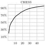
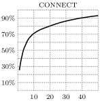
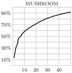
Figure 3: Approximate factorization of Boolean matrices by first 50 factors

A similar tendency can also be observed for graded incidence data. For instance, we have utilized the algorithm in factor analysis of the FOREST FIRES [8] dataset from the UCI Machine Learning Repository. In its original form, the dataset contains real values. It has been therefore transformed into a graded incidence matrix representing relationship between spatial coordinates within the Montesinho park map (rows) and 50 different groups of environmental and climate conditions (columns). The matrix entries are degrees (coming from an equidistant Łukasiewicz chain $L=\{\frac{n}{100}\,|\,n\text{ is integer, }0\leq n\leq 100\}$) to which there has been a large area of burnt forest in the sector of the map under the environmental conditions. Factor analysis of data in this form can help reveal factors which contribute to forests burns in the park. The exact factorization has revealed 46 factors which explain 50 attributes. As in case of the Boolean datasets, relatively small number of factors explain large portions of the data. For instance, more than $50\%$ of the data is covered by $10$ factors, more than $80\%$ of the data is covered by $23$ factors, see Fig. 4.

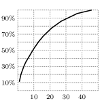
Figure 4: Factorization of graded incidence matrix FOREST FIRES

5 Conclusions

We presented a novel approach to decomposition and factor analysis of matrices with grades, i.e. of a particular form of ordinal data. The factors in this approach correspond to formal concepts in the data matrix. The approach is justified by a theorem according to which optimal decompositions are attained by using formal concepts as factors. The relationship between the factors and original attributes is a non-linear one. An advantageous feature of the model is a transparent way of treating the grades which results in good interpretability of factors. We observed that the decomposition problem is NP-hard as an optimization problem. We proposed a greedy algorithm for computing suboptimal decompositions and provided results of experiments demonstrating its behavior. Furthermore, we presented a detailed example of factor discovery which demonstrates that the method yields interesting factors from data. Since the method developed naturally allows for a linguistic interpretation of factors, it may be considered as a step toward what might be regarded a linguistic factor analysis of qualitative data.

Future research will include the following topics. First, a comparison, both theoretical and experimental, to other methods of matrix decompositions, in particular to the methods emphasizing good interpretability, such as non-negative matrix factorization [17]. Second, an investigation of approximate decompositions of $I$, i.e. decompositions to $A$ and $B$ for which $A\circ B$ is approximately equal to $I$ with respect to a reasonable notion of approximate equality. Third, development of further theoretical insight focusing particularly on reducing further the space of factors to which the search for factors can be restricted. Fourth, study the computational complexity aspects of the problem of approximate factorization, in particular the approximability of the problem of finding decompositions of matrix $I$ [2]. Fifth, explore further the applications of the decompositions studied in this paper, particularly in areas such as psychology, sports data, or customer surveys, where ordinal data is abundant.

References

- [1]
- [2] Ausiello G. et al.: Complexity and Approximation. Combinatorial Otpimization Problems and Their Approximability Properties. Springer, 2003.
- [3] Belohlavek R.: Fuzzy Galois connections. Math. Logic Quarterly 45(4)(1999), 497–504.
- [4] Belohlavek R.: Concept lattices and order in fuzzy logic. Annals of Pure and Applied Logic 128(1–3)(2004), 277–298.
- [5] Belohlavek R.: Optimal decompositions of matrices with entries from residuated lattices. J. Logic and Computation 22(6)(2012), 1405–1425.
- [6] Belohlavek R., Vychodil V.: Discovery of optimal factors in binary data via a novel method of matrix decomposition. J. Computer and System Sciences 76(1)(2010), 3–20.
- [7] Cormen T. H., Leiserson C. E., Rivest R. L., Stein C.: Introduction to Algorithms, 2nd Ed. MIT Press, 2001.
- [8] Cortez P., Morais A.: A Data Mining Approach to Predict Forest Fires using Meteorological Data. In: J. Neves, M. F. Santos and J. Machado Eds., New Trends in Artificial Intelligence, Proc. 13th EPIA 2007, Guimaraes, Portugal, pp. 512–523, 2007.
- [9] Frolov A. A., Húsek D., Muraviev I. P., Polyakov P. A.: Boolean factor analysis by Hopfield-like autoassociative memory. IEEE Transactions on Neural Networks 18(3)(2007), 698–707.
- [10] Ganter B., Wille R.: Formal Concept Analysis. Mathematical Foundations. Springer, Berlin, 1999.
- [11] Geerts F., Goethals B., Mielikäinen T.: Tiling Databases. Proc. DS 2004, Lecture Notes in Computer Science 3245, pp. 278–289.
- [12] Gottwald S.: A Treatise on Many-Valued Logic. Studies in Logic and Computation, vol. 9, Research Studies Press: Baldock, Hertfordshire, England, 2001.
- [13] Hájek P.: Metamathematics of Fuzzy Logic. Kluwer, Dordrecht, 1998.
- [14] Klir G. J., Yuan B.: Fuzzy Sets and Fuzzy Logic. Theory and Applications. Prentice-Hall, 1995.
- [15] Klement E. P., Mesiar R., Pap E.: Triangular Norms. Kluwer, Dordrecht, 2000.
- [16] Krantz H. H., Luce R. D., Suppes P., Tversky A.: Foundations of Measurement. Vol. I (Additive and Polynomial Representations), Vol. II (Geometric, Threshold, and Probabilistic Represenations), Vol. III (Represenations, Axiomatization, and Invariance). Dover Edition, 2007.
- [17] Lee D., Seung H.: Learning the parts of objects by non-negative matrix factorization. Nature 401(1999), 788–791.
- [18] Leeuw J. D.: Principal component analysis of binary data. Application to roll-call analysis, 2003 [Online]. Available at: http://gifi.stat.ucla.edu.
- [19] Mickey M. R., Mundle P., Engelman L.: Boolean factor analysis. In: W.J. Dixon (Ed.), BMDP statistical software manual, vol. 2, 849–860, Berkeley, CA: University of California Press, 1990.
- [20] Miettinen P., Mielikäinen T., Gionis A., Das G., Mannila H.: The Discrete Basis Problem. Proc. PKDD 2006, Lecture Notes in Artificial Intelligence 4213, pp. 335–346.
- [21] Miller G. A.: The magical number seven, plus or minus two: Some limits on our capacity for processing information. Psychol. Rev. 63(1956), 81–97.
- [22] Nau D. S.: Specificity covering: immunological and other applications, computational complexity and other mathematical properties, and a computer program. A. M. Thesis, Technical Report CS–1976–7, Computer Sci.Dept., Duke Univ., Durham, N. C., 1976.
- [23] Nau D. S., Markowsky G., Woodbury M. A., Amos D. B.: A Mathematical Analysis of Human Leukocyte Antigen Serology. Math. Biosciences 40(1978), 243–270.
- [24] Roweis S. T., Saul L. K.: Nonlinear dimensionality reduction by locally linear embedding. Science 290(2000), 2323–2326.
- [25] Sajama, Orlitsky A.: Semi-parametric Exponential Family PCA. In: L. K. Saul, Y.Weiss, L. Bottou (Eds.): Advances in Neural Information Processing, NIPS 2005, Cambridge, MA, pp. 1177–1184.
- [26] Schein A., Saul L., Ungar L.: A generalized linear model for principal component analysis of binary data. Proc. Int. Workshop on Artificial Intelligence and Statistics, pages 14–21, 2003.
- [27] Stockmeyer L. J.: The set basis problem is NP-complete. IBM Research Report RC5431, Yorktown Heights, NY, 1975.
- [28] Tang F., Tao H.: Binary principal component analysis. Proc. British Machine Vision Conference 2006, pp. 377–386, 2006.
- [29] Tatti N., Mielikäinen T., Gionis A., Mannila H.: What is the dimension of your binary data? In: The 2006 IEEE Conference on Data Mining (ICDM 2006), IEEE Computer Society, 2006, pp. 603–612.
- [30] Tenenbaum J. B., de Silva V., Langford J. C.: A global geometric framework for nonlinear dimensionality reduction. Science 290(2000), 2319–2323.
- [31] Vaidya J., Atluri V., Guo Q.: The Role Mining Problem: Finding a Minimal Descriptive Set of Roles. ACM Symposium on Access Control Models and Technologies, June, 2007, pp. 175–184.
- [32] Ward M., Dilworth R. P.: Residuated lattices. Trans. Amer. Math. Soc. 45 (1939), 335–354.
- [33] Zadeh L. A.: Fuzzy sets. Inf. Control 8(1965), 338–353.
- [34] Zivkovic Z., Verbeek J.: Transformation invariant component analysis for binary images. 2006 IEEE Computer Society Conference on Computer Vision and Pattern Recognition, Vol. 1 (CVPR’06), pp. 254–259.