Fast Diffusion of Magnetic Field in Turbulence and Origin of Cosmic Magnetism

Abstract

Turbulence is believed to play important roles in the origin of cosmic magnetism. While it is well known that turbulence can efficiently amplify a uniform or spatially homogeneous seed magnetic field, it is not clear whether or not we can draw a similar conclusion for a localized seed magnetic field. The main uncertainty is the rate of magnetic field diffusion on scales larger than the outer scale of turbulence. To measure the diffusion rate of magnetic field on those large scales, we perform a numerical simulation in which the outer scale of turbulence is much smaller than the size of the system. We numerically compare diffusion of a localized seed magnetic field and a localized passive scalar. We find that diffusion of the magnetic field can be much faster than that of the passive scalar and that turbulence can efficiently amplify the localized seed magnetic field. Based on the simulation result, we construct a model for fast diffusion of magnetic field. Our model suggests that a localized seed magnetic field can fill the whole system in $\sim L_{sys}/L$ times the large-eddy turnover time and that growth of the magnetic field stops in $\sim\max(15,L_{sys}/L)$ times the large-eddy turnover time, where $L_{sys}$ is the size of the system and $L$ is the driving scale. Our finding implies that, regardless of the shape of the seed field, fast magnetization is possible in turbulent systems, such as large-scale structure of the universe or galaxies.

I Introduction

Magnetic fields are ubiquitous in the universe (see, e.g., Name (2013, 2013)). However, origin of magnetic fields in the universe is still an unsolved problem. The origin of cosmic magnetism can be split into two parts - the origin of seed fields and their amplification. In this paper, we are mainly concerned with the latter in the presence of turbulence.

Two extreme types of seed fields can exist - spatially homogeneous and spatially localized ones. If the seed magnetic fields have cosmological origins, it is likely that their coherence lengths are larger than the size of galaxy clusters Rees87; BraEO96 and we can treat them as spatially uniform. It is well known that turbulence can efficiently amplify such a uniform seed field Name (2013, 2013, 2013, 2013, 2013, 2013, 2013, 2013, 2013, 2013, 2013). When we introduce a weak uniform (or homogeneous) magnetic field in a turbulent medium, amplification of the field happens in three stages (see Name (2013); see also Name (2013, 2013)). (1) Exponential growth: Stretching of magnetic field lines occurs most actively near the velocity dissipation scale (i.e. the Kolmogorov scale) first, and the magnetic energy grows exponentially. Note that eddy turnover time is shortest at the scale. (2) Linear growth: The exponential growth stage ends when the magnetic energy becomes comparable to the kinetic energy at the dissipation scale. The subsequent stage is characterized by a linear growth of magnetic energy and a gradual increase of the stretching scale. (3) Saturation: The amplification of magnetic field stops when the magnetic energy density becomes comparable to the kinetic energy density and a final, statistically steady, saturation stage begins.

On the other hand, if the seed fields are ejected from astrophysical bodies, such as active galactic nuclei or galaxies, they will be highly localized in space. Recently Cho & Yoo Name (2013) showed that turbulence can also efficiently disperse and amplify a localized seed magnetic field in an extreme case that the outer scale of turbulence is comparable to the size of the system. However, since their results are valid only for the case the outer scale of turbulence is comparable to the size of the system, their result does not guarantee fast magnetic diffusion in general circumstances.

In this paper, we investigate whether diffusion of magnetic field in turbulence is in general fast. For this purpose, we first perform a numerical simulation in which the outer scale of turbulence is very small. If the outer scale of turbulence is much smaller than the size of the system, it is not clear whether diffusion of magnetic field is fast on scales larger than the outer scale of turbulence. If we consider a passive scalar field, we know that diffusion of the scalar field on scales larger than the outer scale of turbulence is slow because its diffusion over uncorrelated eddies is slow. In this paper, we compare diffusion of a magnetic field and a passive scalar field on scales larger than the outer scale and show that diffusion of the former can be much faster. Based on the simulation, we construct a physical model for fast diffusion of magnetic field in turbulence and apply the model for the large-scale structure of the universe.

We describe numerical method in Section II and theoretical consideration in Section III. We present results in Section IV and discussion and summary in Section V.

Figure 1: Evolution of turbulence before the seed magnetic field is switched on. We start a hydrodynamic turbulence simulation at t$\sim$-12. We run the simulation without a magnetic field for more than 10 large-eddy turnover times. Then we inject a localized seed magnetic field at t=0. The inset shows kinetic energy spectra at 3 time points.

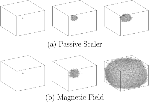
Figure 2: Diffusion of the passive scalar field (upper panels) and the magnetic field (lower panels) at t=0, 11.5, and 28.5 (from left to right). At t=0, the fluid is fully turbulent and the magnetic field and the passive scalar field exist only at the central part of the simulation box. The driving scale ($L$) is about 1/20 of a side of the box ($L_{sys}$).

II Numerical Method

Numerical code — We use a pseudospectral code to solve the incompressible magnetohydrodynamic (MHD) equations in a periodic box of size $2\pi$ ($\equiv L_{sys}$):

$$\frac{\partial{\bf v}}{\partial t}=(\nabla\times{\bf B})\times{\bf B}-(\nabla\times{\bf v})\times{\bf v}+\nu\nabla^{2}{\bf v}+{\bf f}+\nabla P^{\prime},\hskip 14.22636pt$$ (1)

$$\frac{\partial{\bf B}}{\partial t}=\nabla\times({\bf v}\times{\bf B})+\eta\nabla^{2}{\bf B},\hskip 28.45274pt$$ (2)

where $\nabla\cdot{\bf v}=\nabla\cdot{\bf B}=0,$ $\bf{f}$ is random driving force, $P^{\prime}\equiv P+v^{2}/2$, ${\bf v}$ is the velocity, and ${\bf B}$ is magnetic field divided by $(4\pi\rho)^{1/2}$. We also solve the continuity equation for a passive scalar field. We use 100 forcing components in the wavenumber range $15<k<26$, which means the driving scale $L$ is $\sim L_{sys}/20$. In our simulation, $v\sim$1.2 and $\sim$1 before and after saturation, respectively (see Figure 3(d)). Therefore, the large-eddy turnover time, $\sim L/v$, is approximately $\sim$0.26 and $\sim$0.31, respectively. In what follows, we represent time in units of $L/v$ before saturation. Other variables have their usual meaning. We use $512^{3}$ collocation points.

We use hyperviscosity and hyperdiffusion for dissipation terms. The power of hyperviscosity is set to 3, such that the dissipation term in Equation (1) is replaced with $-\nu_{3}(\nabla^{2})^{3}{\bf v}.$ The same expression is used for the magnetic dissipation term with $\eta_{3}=\nu_{3}$ Therefore, the magnetic Prandtl number ($=\nu/\eta$) is one. Since we use hyperviscosity and hyperdiffusion, dissipation of both fields is negligible for small wavenumbers and it abruptly increases near $(2/3)k_{max}$, where $k_{max}$=256 .

Initial conditions — We inject a localized seed magnetic field in a turbulent medium at t=0. In terms of the numerical process, this is achieved in the following way. First, we start off a hydrodynamic turbulence simulation at t$\sim$-12 with zero velocity field (Figure 1). Then, we run the simulation without the magnetic field until it reaches a steady state. The kinetic energy density and spectra in Figure 1 show that the system has reached a statistically steady state before t=0. At t=0, the localized seed magnetic field gets “switched on”.

At $t=0$, the magnetic field has a doughnut shape, which mimics a magnetic field ejected from an astrophysical body. We use the following expression for the magnetic field at t=0:

$${\bf B}(\Delta x,r_{\bot})=\frac{B_{max}}{2\sigma_{0}^{2}e^{-1}}r_{\bot}^{2}e^{-r_{\bot}^{2}/2\sigma_{0}^{2}}e^{-\Delta x^{2}/8\sigma_{0}^{2}}\hat{\bf\theta}_{\perp},$$ (3)

where $B_{max}=0.01$, $\sigma_{0}=4\sqrt{2}$, $r_{\bot}=(\Delta y^{2}+\Delta z^{2})^{1/2}$, and $\Delta x,\Delta y,$ and $\Delta z$ are distances measured from the center of the numerical box in grid units. The unit vector $\hat{\theta}_{\perp}$ is perpendicular to $(\Delta x,0,0)$ and $(0,\Delta y,\Delta z)$. Note that the maximum strength of the magnetic field at t=0 is $B_{max}$. Since $\sigma_{0}=4\sqrt{2}$ in Equation (3), the size of the magnetized region at t=0 is $\sim$16 in grid units, which is $\sim$1/32 of the simulation box size. Therefore, in a cluster of size $\sim$1Mpc, the size of the initially magnetized region corresponds to $\sim$30kpc.

III Theoretical considerations

At t=0, the magnetized region ($\sim$16 in grid units) is smaller than an outer-scale eddy ($\sim$25 in grid units). Since the initial magnetic field is very weak, the magnetic field will be passively advected by turbulent motions inside an outer-scale eddy. Therefore, on scales smaller than the outer scale of turbulence, evolution of the magnetic field is expected to be very similar to that of a passive scalar. Indeed, the standard deviation $\sigma$ of the magnetic field distribution follows the Richardson’s law ($\sigma\propto t^{3/2}$) on scales smaller than the outer scale Name (2013).

On scales larger than the outer scale of turbulence, the passive scalar will diffuse over uncorrelated eddies. Therefore, we expect that $\sigma\propto t^{1/2}$. Then, will the magnetic field follow the same law? This is the question we try to answer in this paper.

IV Results

Results — Figure 2 shows distribution of the passive scalar (upper panels) and $B^{2}$ (lower panels) at t=0, 11.5, and 28.5. At t=0, we set the value of the passive scalar to $B^{2}({\bf x})$. Therefore, both the passive scalar and $B^{2}$ have the same shape at t=0. In the figure we show the regions that satisfy $s({\bf x})\geq 0.6\bar{s}_{c},$ where $\bar{s}_{c}$ is the average value of $s({\bf x})$ inside a sphere of radius 12 (in grid units) at the center of the simulation box. Here $s({\bf x})$ stands for either the passive scalar or $B^{2}$ at ${\bf x}$.

At t=11.5, the magnetic field (lower-middle panel) seems to have a wider distribution than the passive scalar (upper-middle panel). However, calculation shows that their standard deviations are virtually same (see Figure 3(a); compare two curves at t=11.5). The reason the magnetic field looks wider than the passive scalar is that the magnetic field has spatially more intermittent structures. That is, the shaded regions for the magnetic field are more porous than those for the passive scalar. At t=28.5, the magnetic field (lower-right panel) clearly has a much wider distribution than the passive scalar (upper-right panel). Figure 3(a) shows that the standard deviation of the magnetic field is indeed larger than that of the passive scalar at t=28.5.

Figure 3(a) shows that the passive scalar (dashed line) and the magnetic field (solid line) spread similarly until $t\sim$12. The inset shows that both of them follow the $t^{1/2}$ law for $t\lesssim 12$. Note that, since the outer scale is not much larger than the initially magnetized region ($\sim$16 in grid units), we are not able to observe the Richardson’s law: we only observe the $t^{1/2}$ law that happens when the fields diffuse over uncorrelated eddies. Then, at $t\sim$12 the behavior of the two fields suddenly diverges. The passive scalar continues to follow the $t^{1/2}$ law. But, the magnetic field follows a $t^{1}$ law after $t\sim$12.

The slope of $\sigma(t)/L_{sys}$ of magnetic field after $t>12$ in Figure 3(a) is $\sim$1/50. Therefore we can write $\sigma(t)/L_{sys}\sim(1/50)[t/(L/v)]$, or

$$\sigma(t)/L\sim 0.4t/(L/v),$$ (4)

which implies that the spreading speed of the magnetized region (size $\sim$2$\sigma$) is approximately $v$.

Figure 3: (a) The standard deviation ($\sigma$) of the passive scalar (dashed line) and the magnetic field (solid line). Note that $\sigma$ of the magnetic field shows linear increase for $t\gtrsim 12$. (b) The average of $B^{2}$ at the central part of the simulation box. The vertical dashed lines roughly delineate three stages of the magnetic field growth at the center: It follows in turn exponential (I), linear (II) and saturation (III) stages, just as a uniform magnetic field does. Note that it reaches the saturation stage in 15-20 large-eddy turnover times. (c) Same as (b). The vertical axis in drawn in a logarithmic scale. (d) Time evolution of $v^{2}$ and $B^{2}$.

Figure 4: (Left) Schematic explanation. In the ‘magnetized region’, magnetic energy density is larger than the dissipation-scale kinetic energy density and the magnetic field is in either the linear growth stage or the saturation stage. The outer region is not magnetized. The lower graph schematically shows the cross-sectional profile of the magnetic energy density. (Middle) Profile of $<B^{2}(r)>$, where $r$ is the distance from the center of the simulation box. (Right) Timescales in a filament and clusters. The large-eddy turnover time is $\sim L/v$. Magnetization timescale ($t_{mag}$) is the timescale for magnetic field to fill the whole system and is equal to $\sim(L_{sys}/L)(L/v)$. Saturation timescale ($t_{sat}$) is the timescale for the central magnetic field to reach the saturation stage and is equal to $\sim$15$L/v$.

Why is this happening? Figure 3(b) gives us a useful hint. Initially $<B_{c}^{2}>$, the average of $B^{2}$ inside a sphere of radius 24 (in grid units) at the center of the simulation box, shows exponential growth (see Figure 3(c)). Then $<B_{c}^{2}>$ shows roughly a linear growth for $12\lesssim t\lesssim 20$ (see Figure 3(b)). After $t\gtrsim 20$, $<B_{c}^{2}>$ becomes saturated. This 3-stage growth is very similar to the growth of a uniform seed magnetic field.

Model — We note that the beginning of the linear growth stage for $<B_{c}>$ almost coincides with the divergence of the behavior of the two fields in Figure 3(a). Based on this observation and the 3-stage growth model for a uniform seed magnetic field (see Name (2013, 2013)), we can construct a model for a localized seed magnetic field.

First, when the magnetic field is very weak so that magnetic back-reaction is negligible, the magnetic energy grows exponentially, which is due to stretching of magnetic field lines at the dissipation scale. During this stage, diffusion of magnetic field is very similar to that of the passive scalar. In our simulation, this stage ends at $t\sim$12.

Second, as the magnetic energy density in the central region reaches the kinetic energy density at the dissipation scale, the exponential growth stage ends due to suppression of stretching at the dissipation scale and a slower linear growth stage begins in the central region. Note however that the linear growth begins only in the central region. Magnetic field still grows exponentially in other regions. As the magnetic field in the central region grows slowly, the distribution of magnetic field may look like the graph in the left panel of Figure 4. The width of the flat central part increases linearly in time. This can be understood as follows. Consider an outer-scale eddy on the boundary of the central region (see eddy A in the left panel of Figure 4). As shown in the figure, some part of the eddy is magnetized and the rest of the eddy is not magnetized. We know that magnetic diffusion inside an outer-scale eddy is very fast: it takes roughly one eddy turnover time for magnetic field to fill the whole eddy Name (2013). Therefore, after approximately one large-eddy turnover time, the whole eddy becomes magnetized. This way, we have a linear widening (or ‘expansion’) rate and the speed of expansion is of order $\sim v$, the large-scale velocity . During this stage the standard deviation of magnetic field distribution, which measures the size of the flat central region, grows linearly in time and the magnetic energy density will be proportional to $\sigma^{3}<B^{2}_{c}>\propto t^{4}$.

Third, depending on the strength of the seed field and the ratio $L_{sys}/L$, either the magnetic field fills the whole system first or the central magnetic field reaches the saturation stage first. In our simulation the latter happens first at $t\sim$15-20 (see Figure 3(b)). In this case, the standard deviation of magnetic field distribution continues to grow linearly in time and the magnetic energy density becomes proportional to $\sim\sigma^{3}\propto t^{3}$. Finally, when the magnetic field fills the whole system the growth stage ends (Figure 3(d)). On the other hand, if the magnetic field fills the whole system first, the subsequent evolution of magnetic field will be very similar to the linear grow stage of a spatially homogeneous/uniform seed field case.

The middle panel of Figure 4 shows cross-sectional profile of $B^{2}$. When $t\lesssim 12$, magnetic energy density at the center grows exponentially. At the same time, the width of the profile increases slowly: $\sigma(t)\propto t^{1/2}$. At $t\sim$12, the central magnetic energy density becomes comparable to the kinetic energy density at the dissipation scale and the exponential growth stops. After $t\sim$12, the central magnetic field grows slowly and the width of the flat central part increases. The overall behavior of the cross-sectional magnetic field profile is consistent with our model.

V Discussion and Summary

Discussion — In this paper, we have found that, during the linear expansion stage, the speed at which magnetized region expands is of order $\sim v$. Therefore, it will take

$$t_{mag}\sim L_{sys}/v=(L_{sys}/L)(L/v)$$ (5)

for magnetic field to fill the whole system. On the other hand, in the limit of vanishing $\nu~{}(=\eta)$, any weak magnetic field at the center can reach the saturation stage in about 15 large-eddy turnover times, so that we take

$$t_{sat}\sim 15(L/v),$$ (6)

which is the same as the saturation timescale for a uniform seed field case (see, for example, Name (2013, 2013, 2013); see also Figure 3(b)). If $t_{sat}<t_{mag}$ (or, $L_{sys}/L\gtrsim 15$), magnetic field at the center reaches saturation first and growth of magnetic field ends when it fills the whole system, just as in our simulation. If $t_{sat}>t_{mag}$ (or, $L_{sys}/L\lesssim 15$), magnetic field fills the whole system first and continues to grow until it reaches the saturation stage. In this case, the behavior of the system after $t_{mag}$ will be very similar to that of a uniform seed field case. In general, the growth of magnetic field ends in $t\sim\max(t_{mag},t_{sat})=\max(15,L_{sys}/L)(L/v)$.

In the large-scale structure of the universe, the driving scale of turbulence is uncertain (see references in Name (2013)). Here, we calculate timescales for three possible examples related to the large-scale structure of the universe. We plot the timescales in the right panel of Figure 4. We use $L_{sys}=3Mpc$, $L=500kpc$, $v=150km/s$ for a filament, $L_{sys}=1Mpc$, $L=400kpc$, $v=300km/s$ for a cluster with large-scale driving, and $L_{sys}=1Mpc$, $L=50kpc$, $v=100km/s$ for a cluster with small-scale driving. The figure shows that the magnetization timescales for those systems are either comparable to or shorter than the age of the universe. Therefore, we expect that most volumes in those systems are filled with magnetic fields. Magnetic field in the filament will be very weak, because it is in early stage of magnetic field growth. Magnetic fields in clusters will be relatively strong: the cluster with large-scale driving ($L=L_{sys}/2.5$) has almost reached the saturation stage and the cluster with small-scale driving ($L=L_{sys}/20$) has already reached the saturation stage.

The right panel of Figure 4 implies that it is difficult to tell whether the origin of the seed magnetic field is cosmological or astrophysical if we observe galaxy clusters. However, if we observe filaments, it could be possible to tell the origin of the seed magnetic field because filaments may be partially magnetized if the origin is astrophysical and if there are not many sources.

In this paper, we have assumed that the viscosity $\nu$ is very small, so that the Reynolds number ($Lv/\nu$) is very large. However, there are claims that viscosity in intracluster medium is non-negligible Name (2013, 2013, 2013, 2013). If this is the case, what will happen when we inject a weak localized seed magnetic field at the center of a numerical box? Of course, it depends on the value of $L/L_{sys}$. Since the case of $L\sim L_{sys}$ was discussed in Cho & Yoo Name (2013), let us focus on the case of small $L/L_{sys}$ in this paper. In particular, let us assume that the seed magnetic field initially grows exponentially and that the value of $L/L_{sys}$ is so small that magnetic field at the central region reaches either a linear growth stage or a saturation stage before the magnetic field fills the whole system. If the Reynolds number is less than $\sim O(10^{3})$, the outer scale and the dissipation scale of velocity field are so close that the growth of the magnetic field is dominated by the exponential growth stage. That is, the central magnetic field will grow exponentially most of the time and, if any, there will be very short linear growth stage Name (2013). During the exponential growth stage, the magnetic field is passively advected by the outer-scale eddy motions. Therefore, the behavior of the magnetic field will be very similar to that of a passive scalar, which means that diffusion of magnetic field on scales larger than the outer scale is very slow and follows a $t^{1/2}$ law. After the exponential growth stage ends, the magnetic field will show a linear expansion. The total time for the system to reach a fully magnetized saturation stage will be the sum of the duration of the exponential growth stage and $\sim L_{sys}/v$. However, it is not easy to estimate the time because the duration of the exponential growth stage depends on the strength of the seed magnetic field.

Summary — In this paper, we have shown that magnetic diffusion is very fast in a turbulent medium even on scales larger than the outer scale of turbulence. When we inject a weak localized seed magnetic field at the center of a turbulent medium, it initially grows exponentially by stretching of magnetic field lines near the dissipation scale and fills the outer-scale eddy at the center very fast. After filling the outer-scale eddy, diffusion rate slows down ($\sigma\propto t^{1/2}$) because the magnetic field diffuses over uncorrelated outer-scale eddies. At this stage, diffusion of the magnetic field is similar to that of a passive scalar. Then, as the central magnetic field reaches energy equipartition with dissipation-scale velocity field, the standard deviation of the magnetic field begins to show a faster growth rate. At this stage, the speed at which the magnetized region ‘expands’ is of order $\sim v$, which enables a full magnetization of the system in a timescale of $\sim L_{sys}/v$.

In the limit of $\nu$ (=$\eta$) $\rightarrow 0$, growth of a localized seed magnetic field ends in $\sim\max(15,L_{sys}/L)(L/v)$. Note that earlier studies Name (2013, 2013) have shown that turbulence can efficiently amplify a spatially uniform or homogeneous seed field, the timescale of which is $\sim 15(L/v)$. Therefore, unless $L_{sys}/L$ is extremely large, we can conclude that turbulence can amplify any shape of seed magnetic field very fast.