Massive non-planar two-loop four-point integrals with SecDec 2.1

Abstract

We present numerical results for massive non-planar two-loop box integrals entering heavy quark pair production at NNLO, some of which are not known analytically yet. The results have been obtained with the program SecDec 2.1, based on sector decomposition and contour deformation, in combination with new types of transformations. Among the new features of version 2.1 is also the possibility to evaluate contracted tensor integrals, with no limitation on the rank.

PACS: 12.38.Bx, 02.60.Jh, 02.70.Wz

MPP-2013-48

,

1 Introduction

There are a few processes measured at the LHC where the need for corrections beyond next-to-leading order (NLO) is free of doubt. One of them is top quark pair production, and the completion of a full NNLO prediction is well under way [1, 2, 3, 4, 5, 6, 7, 8, 9, 10, 11, 12, 13]. Soft gluon and Coulomb effects also have been taken into account beyond the next-to-leading logarithmic accuracy and have been combined with fixed order results to come up with predictions as precise as possible [14, 15, 16, 17, 18, 19, 20, 21].
Among the key ingredients of the full NNLO calculation are the master integrals entering the two-loop virtual corrections. While in [22, 23, 24] the latter enter in a semi-numerical form, a fully analytical representation for a subset of the needed master integrals has been presented in [4, 5, 6], where the fermionic and leading colour contributions to the $q\bar{q}$ channel and the leading colour contributions to the $gg$ channel are calculated. An analytical representation for the non-planar seven-propagator integral occurring in the light fermionic correction to the $gg$ channel also has been achieved [7, 8]. However, explicit results for some of the most complicated non-planar master integrals are still missing.

Here we present numerical results for two non-planar seven-propagator topologies, one entering the light fermionic correction to the $gg$ channel, where analytical results exist [7, 8], the other one entering the heavy fermionic correction to the $gg$ channel, where no analytical result is available yet. Apart from scalar master integrals, we also give results for an irreducible tensor integral of rank two for the diagram entering the heavy fermionic correction to the $gg$ channel. In order demonstrate the applicability of the tensor option to various types of integrals, we also calculate some two-loop two-point functions involving several different mass scales and show that the timings for the tensor integrals are not much larger than the ones for the scalar integrals. This means that a numerical approach in certain cases can help to alleviate or even avoid the procedure of amplitude reduction to master integrals.

The results have been obtained with the program SecDec  2.1 [25, 26, 27], based on sector decomposition to disentangle the singularity structure, followed by numerical contour integration. Compared to version 2.0 of SecDec  , version 2.1 contains a number of new features, which are also presented in this article. Among them is the possibility to evaluate tensor integrals with (in principle) no limitation on the rank. Another new feature is the option to apply the sector decomposition algorithm and subsequent contour deformation on user-defined functions which do not necessarily have the form of standard loop integrals. In fact, to achieve a convenient representation for one of the seven-propagator integrals, some analytical manipulations have been done before starting the algorithm, this way reducing the number of produced subsectors, leading to improved numerical behaviour.

The structure of this article is as follows. In Section 2 we will derive the expression serving as a starting point for the evaluation of the massive non-planar two-loop box diagram mentioned above, and describe novel types of transformations which can be used to reduce the number of sector decompositions. The new features of the program SecDec  2.1 are discussed in Section 3. Numerical results are presented in Section 4, where we also give results for some rank three tensor integrals for massive two-point functions. An appendix contains a manual-style description of the new features of the program. Detailed documentation of the program also comes with the code, which is available at http://secdec.hepforge.org.

2 Analytic preparation of the master diagrams

The structure and usage of SecDec  and the procedures it uses are described in detail in Refs. [25, 26, 28, 29]. The main purpose of this section is to explore the possibilities arising from a mixed approach, where simple analytic manipulations to the integral before feeding it to the sector decomposition algorithm can lead to a large gain in efficiency for the subsequent numerical evaluation.

2.1 Non-planar seven propagator integrals with two massive on-shell legs

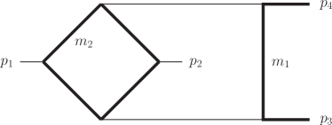
(a) ggtt1

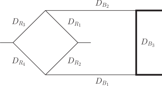
(b) ggtt2

Figure 1: Massive non-planar two-loop box diagrams entering the heavy (a) and light (b) fermionic correction to the $gg$ channel; the thick lines denote massive particles.

The diagrams shown in Fig. 1 are master topologies occurring in the two-loop corrections to $t\bar{t}$ production in the $gg$ channel. While results for the diagram corresponding to massless fermionic corrections in a sub-loop – which we call ggtt2 – are available in terms of ${\cal O}(800)$ generalized polylogarithms [7], analytic results for the integral ggtt1, containing a sub-diagram with a massive loop, are not available. Numerically however, the evaluation of ggtt1 is easier than the one of ggtt2, due to its less complicated infrared singularity structure. While the leading poles of ggtt2 are of order $1/\epsilon^{4}$, and intermediate expressions during sector decomposition show (spurious) pole structures where the degree of divergence is higher than logarithmic, the integral ggtt1 has only finite contributions. Therefore we evaluate ggtt1 with SecDec   2.1 fully automatically, while for ggtt2 it is advantageous to make some analytical manipulations beforehand, reducing both, the number of Feynman parameters to be integrated over numerically and the degree of divergence.

The expression for the scalar integral ggtt2 in momentum space is given by

$$\mathcal{G}_{ggtt2}=\left(\frac{1}{\mathrm{i}\pi^{\frac{\mathrm{D}}{2}}}\right)^{2}\int\frac{\mathrm{d^{D}}k_{1}\,\,\mathrm{d^{D}}k_{2}}{D_{R_{1}}D_{R_{2}}D_{R_{3}}D_{R_{4}}D_{B_{1}}D_{B_{2}}D_{B_{3}}}$$ (1)

where $\mathrm{D}=4-2\epsilon$. The Feynman propagators $D_{R_{i}}$ corresponding to the “rhombus” sub-loop in Fig. 1 are given by

$$D_{R_{1}} =(k_{1}-k_{2})^{2}+\mathrm{i}\delta\text{ ,}\hskip 15.0ptD_{R_{2}}=(k_{1}-k_{2}+p_{2})^{2}+\mathrm{i}\delta\text{ ,}$$

$$D_{R_{3}} =(k_{2}+p_{4})^{2}+\mathrm{i}\delta\text{ ,}\hskip 15.0ptD_{R_{4}}=(k_{2}+p_{1}+p_{4})^{2}+\mathrm{i}\delta\text{ ,}$$ (2)

where the $p_{i}$ are the external momenta with $p_{3}^{2}=p_{4}^{2}=m^{2}$ and $p_{1}^{2}=p_{2}^{2}=0$, and $k_{1}$, $k_{2}$ are the loop momenta. Integrating out the loop momentum $k_{2}$ first, we are left with an expression containing $k_{1}$ and external momenta only, to be combined with the propagators

$$D_{B_{1}}=(k_{1}-p_{3})^{2}+\mathrm{i}\delta\text{ ,}\hskip 10.0ptD_{B_{2}}=(k_{1}+p_{4})^{2}+\mathrm{i}\delta\text{ ,}\hskip 10.0ptD_{B_{3}}=k_{1}^{2}-m^{2}+\mathrm{i}\delta\;.$$ (3)

The introduction of Feynman parameters for the one-loop subgraph $\mathcal{I}_{R}$ containing only the loop momentum $k_{2}$ leads to

$$\mathcal{I}_{R}=\frac{1}{\mathrm{i}\pi^{\mathrm{D}/2}}\int\frac{\mathrm{d^{D}}k_{2}}{D_{R_{1}}D_{R_{2}}D_{R_{3}}D_{R_{4}}}=\Gamma(2+\epsilon)\int\prod_{i=1}^{4}\mathrm{d}x_{i}\delta(1-\sum_{j=1}^{4}x_{j})\mathcal{F}(\vec{x},k_{1})^{-2-\epsilon}\text{ ,}$$ (4)

with

$$\!\!-\mathcal{F}(\vec{x},k_{1})=D_{B_{1}}x_{1}x_{2}+(k_{1}+p_{1}+p_{4})^{2}x_{1}x_{3}+(k_{1}+p_{2}+p_{4})^{2}x_{2}x_{4}+D_{B_{2}}x_{3}x_{4}\text{ .}$$

We eliminate the $\delta$-function in eq. (4) with the substitution

$$x_{1}=t_{2}(1-t_{3})\text{ ,}\hskip 19.0ptx_{2}=t_{1}t_{3}\text{ ,}\hskip 19.0ptx_{3}=(1-t_{1})t_{3}\text{ ,}\hskip 19.0pt$$ (5)

to achieve a factorisation of the parameter $t_{3}$ which then is integrated out analytically, leading to

$$\mathcal{I}_{R} =-\frac{2}{\epsilon}\frac{\Gamma(2+\epsilon)\Gamma^{2}(1-\epsilon)}{\Gamma(1-2\epsilon)}\int_{0}^{1}\mathrm{d}t_{1}\int_{0}^{1}\mathrm{d}t_{2}\,\,\mathcal{\tilde{F}}(\vec{t},k_{1})^{-2-\epsilon}$$

with

$$-\mathcal{\tilde{F}}(\vec{t},k_{1})=D_{B_{1}}t_{1}t_{2}+(k_{1}+p_{1}+p_{4})^{2}t_{1}\bar{t}_{2}+(k_{1}+p_{2}+p_{4})^{2}\bar{t}_{1}t_{2}+D_{B_{2}}\bar{t}_{1}\bar{t}_{2}\text{ ,}$$ (6)

and where we used the shorthand notation $\bar{t}_{i}=1-t_{i}$. Now we combine the expression for the 1-loop rhombus $\mathcal{I}_{R}$ with the remaining $k_{1}$-dependent propagators, treating the expression of eq. (6) as a fourth propagator with power $2+\epsilon$, to obtain, after integrating out $k_{1}$,

$$\mathcal{G}_{NP}= \frac{2}{\epsilon}\frac{\Gamma(3+2\epsilon)\Gamma^{2}(1-\epsilon)}{\Gamma(1-2\epsilon)}\int_{0}^{1}\mathrm{d}t_{1}\int_{0}^{1}\mathrm{d}t_{2}\,\,\times$$

$$\prod_{i=1}^{4}\int_{0}^{1}\mathrm{d}z_{i}\,z_{4}^{1+\epsilon}\,\delta(1-\sum_{j=1}^{4}z_{j})\,\,\mathcal{F_{NP}}(\vec{z},t_{1},t_{2})^{-3-2\epsilon}\,\,\mathcal{U_{NP}}(\vec{z})^{1+3\epsilon}\text{ ,}$$ (7)

where

$$\mathcal{U_{NP}}(\vec{z}) =\sum_{j=1}^{4}z_{j}\hskip 19.0pt\text{ and}$$

$$\mathcal{F_{NP}}(\vec{z},t_{i}) =-s_{12}z_{2}z_{3}-Tz_{1}z_{4}-S_{1}z_{2}z_{4}-S_{2}z_{3}z_{4}+m^{2}z_{1}(z_{1}+z_{4}Q)\text{ ,}$$ (8)

with

$$T =s_{13}\bar{t}_{1}t_{2}+s_{23}t_{1}\bar{t}_{2}\text{ ,}\hskip 19.0ptS_{1}=s_{12}t_{1}t_{2}\text{ ,}\hskip 19.0ptS_{2}=s_{12}\bar{t}_{1}\bar{t}_{2}$$

$$Q =t_{1}\bar{t}_{2}+\bar{t}_{1}t_{2}\text{ ,}\hskip 19.0pts_{ij}=(p_{i}+p_{j})^{2}\text{ .}$$ (9)

Now we eliminate the $\delta$-function by performing a primary sector decomposition [28] in $z_{1},\dots,z_{4}$ to obtain

$$\mathcal{G}_{NP}= \frac{2}{\epsilon}\frac{\Gamma(3+2\epsilon)\Gamma^{2}(1-\epsilon)}{\Gamma(1-2\epsilon)}\int_{0}^{1}\mathrm{d}t_{1}\int_{0}^{1}\mathrm{d}t_{2}\sum_{i=1}^{4}G_{NP}^{i}\text{ ,}$$ (10)

with

$$G_{NP}^{1} =\int_{0}^{1}\mathrm{d}z_{2}\,\mathrm{d}z_{3}\,\mathrm{d}z_{4}\,\,\,z_{4}^{1+\epsilon}\,\,\,(1+z_{2}+z_{3}+z_{4})^{1+3\epsilon}\,\,\,\mathcal{F}^{1}(\vec{z},t_{i})^{-3-2\epsilon}$$

$$\mathcal{F}^{1}(\vec{z},t_{i}) =-s_{12}z_{2}z_{3}-Tz_{4}-S_{1}z_{2}z_{4}-S_{2}z_{3}z_{4}+m^{2}(1+z_{4}Q)\text{ ,}$$

$$G_{NP}^{2} =\int_{0}^{1}\mathrm{d}z_{1}\,\mathrm{d}z_{3}\,\mathrm{d}z_{4}\,\,\,z_{4}^{1+\epsilon}\,\,\,(1+z_{1}+z_{3}+z_{4})^{1+3\epsilon}\,\,\,\mathcal{F}^{2}(\vec{z},t_{i})^{-3-2\epsilon}$$

$$\mathcal{F}^{2}(\vec{z},t_{i}) =-s_{12}z_{3}-Tz_{1}z_{4}-S_{1}z_{4}-S_{2}z_{3}z_{4}+m^{2}z_{1}(z_{1}+z_{4}Q)\text{ ,}$$ (11)

$$G_{NP}^{3} =\int_{0}^{1}\mathrm{d}z_{1}\,\mathrm{d}z_{2}\,\mathrm{d}z_{4}\,\,\,z_{4}^{1+\epsilon}\,\,\,(1+z_{1}+z_{2}+z_{4})^{1+3\epsilon}\,\,\,\mathcal{F}^{3}(\vec{z},t_{i})^{-3-2\epsilon}$$

$$\mathcal{F}^{3}(\vec{z},t_{i}) =-s_{12}z_{2}-Tz_{1}z_{4}-S_{1}z_{2}z_{4}-S_{2}z_{4}+m^{2}z_{1}(z_{1}+z_{4}Q)\text{ ,}$$

$$G_{NP}^{4} =\int_{0}^{1}\mathrm{d}z_{1}\,\mathrm{d}z_{2}\,\mathrm{d}z_{3}\,\,\,(1+z_{1}+z_{2}+z_{3})^{1+3\epsilon}\,\,\,\mathcal{F}^{4}(\vec{z},t_{i})^{-3-2\epsilon}$$

$$\mathcal{F}^{4}(\vec{z},t_{i}) =-s_{12}z_{2}z_{3}-Tz_{1}-S_{1}z_{2}-S_{2}z_{3}+m^{2}z_{1}(z_{1}+Q)\text{ .}$$ (12)

We observe that $\mathcal{F}^{1}(\vec{z},t_{i})$ is of the form $m^{2}+{\mathrm{func}}(z_{i},t_{i})$, so does not need any further decomposition, and primary sector 3 can be remapped to primary sector 2 by exchanging $z_{2}\leftrightarrow z_{3}$ and $S_{1}\leftrightarrow S_{2}$. Hence, we are left with the treatment of primary sectors 2 and 4 only.
The integrals $G_{NP}^{2,3,4}$ can have singularities both at zero and one in $t_{1}$ and $t_{2}$. With the sector decomposition algorithm, only singularities at zero are factorized automatically. Consequently, we remap the singularities located at the upper integration limit to the origin of parameter space by splitting the integration region at $\tfrac{1}{2}$ and transforming the integration variables to remap the integration domain to the unit cube [29]. This procedure results in 12 integrals, some of which already being finite, such that no subsequent sector decomposition is required. Some of the integrals however lead to singularities of the type $\int_{0}^{1}dx\,x^{-2-\epsilon}$ after sector decomposition, which we call linear singularities. These singularities are spurious and can be subtracted by expanding the Taylor series in the subtraction procedure up to the second term [28, 30]. However, this procedure can lead to large cancellations between subtraction terms and therefore to numerical instabilities. Hence it is advisable to try avoiding this type of singularity from scratch. In the following section we describe a method which can help to do so.

2.2 Removal of double linear divergences via backwards transformation

The aim of the procedure described in this section is to achieve a transformation of potential linear divergences into logarithmic divergences as far a possible. A different procedure towards this goal, based on integration-by-parts identities, has been described in [25]. The latter method however can increase the number of functions to be integrated substantially, while the method described below in general reduces the number of further iterations and therefore the number of produced functions. Yet another method to reduce the number of functions produced during factorization has been suggested in Ref. [31], but we do not use it here as it can introduce singularities at the upper integration limit which subsequently have to be remapped again.

To explain the type of transformation advocated here, we use a function of the structure of $\mathcal{F}^{2}$ in eq. (11) as an example, renaming $t_{2}\to z_{2},t_{1}\to z_{5}$. Concerning the Feynman parameters, we can identify the following structure in eq. (11) (in our concrete example $N=5,z_{j}=z_{4},z_{k}=z_{1}$)

$$I=\prod_{i=1}^{N}\left\{\int_{0}^{1}{\rm d}z_{i}\right\}\,\left[z_{j}\left(P(\vec{z}_{jk})+z_{k}Q(\vec{z}_{jk})\right)+R(\vec{z}_{jk})\right]^{-\alpha}\text{ ,}$$ (13)

where $\alpha$ is assumed to be positive, and where $P,Q$ and $R$ are polynomials of arbitrary degree of the Feynman parameters $\vec{z}_{jk}=(z_{1},\dots,\hat{z}_{j},\dots,\hat{z}_{k},\dots,z_{N})$ and kinematic invariants. The hat denotes Feynman parameters which do not occur in the corresponding function.
In eq. (13), all terms multiplied by the Feynman parameter $z_{k}$ are also multiplied by the Feynman parameter $z_{j}$. Hence, the sector decomposition method can be applied “backwards”. To explain this in more detail, consider the following function:

$$J= \prod_{i=1}^{N}\left\{\int_{0}^{1}{\rm d}z_{i}\right\}\,\frac{1}{z_{j}}\left[z_{j}P(\vec{z}_{jk})+z_{k}Q(\vec{z}_{jk})+R(\vec{z}_{jk})\right]^{-\alpha}[\underbrace{\Theta(z_{k}-z_{j})}_{(1)}+\underbrace{\Theta(z_{j}-z_{k})}_{(2)}]$$ (14)

Now we substitute $z_{j}=z_{k}\,t_{j}$ in sector (1) and $z_{k}=z_{j}\,t_{k}$ in sector (2), to obtain, after renaming again $t_{i}$ into $z_{i}$

$$J =\prod_{i=1}^{N}\left\{\int_{0}^{1}{\rm d}z_{i}\right\}\frac{1}{z_{j}}\left[z_{j}P(\vec{z}_{jk})+z_{k}Q(\vec{z}_{jk})+R(\vec{z}_{jk})\right]^{-\alpha}$$ (15)

$$=\prod_{i=1}^{N}\left\{\int_{0}^{1}{\rm d}z_{i}\right\}\frac{1}{z_{j}}\left[z_{k}(z_{j}P(\vec{z}_{jk})+Q(\vec{z}_{jk}))+R(\vec{z}_{jk})\right]^{-\alpha}$$ (16)

$$\quad+\prod_{i=1}^{N}\left\{\int_{0}^{1}{\rm d}z_{i}\right\}\left[z_{j}(P(\vec{z}_{jk})+z_{k}Q(\vec{z}_{jk}))+R(\vec{z}_{jk})\right]^{-\alpha}\;.$$ (17)

We observe that the term in eq. (17) is the same as eq. (13). Therefore we can replace it by the expressions (15) minus (16). The effect is twofold: The degree of the polynomial in $z_{j}z_{k}$ is reduced in eq. (15), and in eq. (16) the degree of divergence in $z_{j}$ is reduced if $\alpha>1$.
After all transformations of this type we arrive at a total of 15 functions partly needing an iterated sector decomposition. Together with the introduction of the new feature of user-defined functions in SecDec  2.1, which we will describe in the following section, we are now able to compute the ggtt2 diagram in a reasonable amount of time.

3 Structure and new features of SecDec  version 2.1

3.1 Structure

Figure 2: Flowchart showing the main steps the program performs to produce the numerical result as a Laurent series in $\epsilon$.

The workflow of the program is shown in Fig. 2. The directory structure of SecDec  splits into two main branches: loop and general. In the loop part, multi-scale loop integrals can be evaluated without restricting the kinematics to the Euclidean region. Integrable singularities are dealt with by deforming the integration contour into the complex plane. In the general part, the poles of more general parametric functions can be factorized, and subsequently the functions can be evaluated numerically, provided they contain only end-point singularities. Contour deformation is not available in the subdirectory general. For more information on the structure of the various subdirectories we refer to Ref. [26].

3.2 New features

The main new features of SecDec  version 2.1 are the -u option in the loop directory to decompose “user defined” functions rather than standard multi-loop integrals, an extended tensor integral option, and improvements in the error treatment.

Evaluation of user-defined functions with arbitrary kinematics

If the user would like to calculate a “standard” loop integral, it is sufficient to specify the propagators, and the program will construct the integrand in terms of Feynman parameters automatically. However, in section 2 we have seen that an analytical step can be helpful when dealing with complicated integrals. Integrating out one Feynman parameter analytically reduces the number of integration variables for the subsequent Monte Carlo integration and therefore in general improves numerical efficiency. This implies that the constraint $\delta(1-\sum_{i}x_{i})$ has been used already to achieve a convenient parametrisation, and therefore no primary sector decomposition to eliminate the $\delta$-constraint is needed anymore. In such a case, the user can skip the primary sector decomposition step and insert the functions to be factorized directly into the Mathematica input file, using his favourite parametrisation. More generally speaking, the purpose of this option is to be more flexible with regards to the functions to be integrated, such that expressions for loop integrals which are not in the “standard form” – for example due to analytic manipulations which have been performed already on the integral – can be dealt with as well. This includes the possibility to perform a deformation of the integration contour into the complex plane, taking the user-defined functions as a starting point. Oriented at the functions $\mathcal{F}$ and $\mathcal{U}$ for the “standard” loop case (see e.g. eq. (2.1)), the user-defined functions can encompass the product of two arbitrary polynomial functions with different exponents and an additional numerator. Details about the usage of this option are given in appendix A.2.

The tensor integral option and the syntax for the definition of the numerator in terms of contracted loop momenta are described in detail in appendix A.3.

Error estimates

When dealing with complicated integrands it can happen that the error given by the numerical integration program – which is based on the number of sampling points only – underestimates the true error. The numerical integrators contained in the Cuba library [32, 33] give an estimate of the correctness of the stated error to a given result. The new SecDec  version 2.1 collects the maximal error probability for each computed order in the dimensional regulator $\epsilon$ and writes it to the result files *.res. In the generic case, the information on the reliability of the stated error is given as a probability with values between 0 and 1. If the integrator returns a value larger than one, the integration has not come to successful completion, and a warning is written to the result files. This feature helps the user to judge how reliable the numerical results, respectively the given errors, are.

3.3 Installation and usage

The program can be downloaded from http://secdec.hepforge.org.
Unpacking the tar archive via tar xzvf SecDec.tar.gz will create a directory called SecDec with the subdirectories as described above. Installation is done by changing to the SecDec directory and running ./install.

Prerequisites are Mathematica, version 6 or above, Perl (installed by default on most Unix/Linux systems), a C++ compiler, and a Fortran compiler if the Fortran option is used.

Details about the usage can be found in the appendix, where manual-type descriptions of the new features are given, and also in Ref. [26] and the documentation coming with the program.

4 Results

Now we present numerical results for two non-planar seven propagator master topologies occurring in the two-loop corrections to the process $gg\to t\bar{t}$, shown in Fig. 1. In addition to the scalar integrals, we also compute an irreducible tensor integral. In order to demonstrate the applicability of the tensor option to various contexts, we also give results for some rank three tensor two-point functions involving several mass scales.

4.1 The ggtt1 diagram

Numerical results for the diagram ggtt1 (see Fig. 1(a)) are shown in Fig. 3 for both the scalar integral and an irreducible rank two tensor integral.

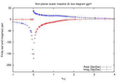
(a) scalar integral

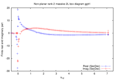
(b) rank 2 tensor integral

Figure 3: Results for the scalar integral ggtt1 shown in Fig. 1(a), and the corresponding rank two tensor integral ggtt1 with $k_{1}\cdot k_{2}$ in the numerator. We vary $s_{12}$ and fix $s_{23}=-1.25,m_{2}=m_{1},p_{3}^{2}=p_{4}^{2}=m_{1}^{2}=1$.

The integral representation of the diagram ggtt1 is given by

$$\mathcal{G}_{ggtt1}= \left(\frac{1}{\mathrm{i}\pi^{\frac{\mathrm{D}}{2}}}\right)^{2}\int\frac{\mathrm{d^{D}}k_{1}\,\mathrm{d^{D}}k_{2}}{D_{1}\ldots D_{7}}\;\,;\,D_{1}=k_{1}^{2}-m_{2}^{2},D_{2}=(k_{1}+p_{1})^{2}-m_{2}^{2},$$ (18)

$$D_{3}=k_{2}^{2}-m_{2}^{2},D_{4}=(k_{2}+p_{2})^{2}-m_{2}^{2},D_{5}=(k_{1}-k_{2}+p_{1})^{2},$$

$$D_{6}=(k_{1}-k_{2}-p_{2})^{2},D_{7}=(k_{1}-k_{2}+p_{1}+p_{3})^{2}-m_{1}^{2}\;,$$

where we omitted the infinitesimal $\mathrm{i}\delta$ in the propagators, and we use the convention that all external momenta are ingoing. The momenta $p_{3}$ and $p_{4}$ are massive on-shell: $p_{3}^{2}=p_{4}^{2}=m_{1}^{2}$. The results shown Fig. 3(b) correspond to the rank two tensor integral with the same propagators and a factor of $k_{1}\cdot k_{2}$ in the numerator. The numerical integration errors are shown as horizontal markers on the vertical lines. The absence of such markers means that the numerical errors are smaller than visible in the plot.

The timings for one kinematic point for the scalar integral in Fig. 3(a) range from 11-60 secs for points far from threshold to $1.6\times 10^{3}$ seconds for a point very close to threshold, with an average of about 500 secs for points in the vicinity of the threshold. A relative accuracy of $10^{-3}$ has been required for the numerical integration, while the absolute accuracy has been set to $10^{-5}$. For the tensor integral, the timings are better than in the scalar case, as the numerator function present in this case smoothes out the singularity structure. A phase space point far from threshold takes about 5-10 secs, while points very close to threshold do not exceed 3600 secs for the rank 2 tensor integral, Fig. 3(b). The timings were obtained on a single machine using Intel i7 processors and 8 cores.

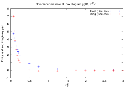
Figure 4: Results for the scalar integral ggtt1 shown in Fig. 1(a), with two different masses. We vary $m_{2}$ and fix $s_{12}=5,s_{23}=-1.25,p_{3}^{2}=p_{4}^{2}=m_{1}^{2}=1$.

For the results shown in Fig. 3 we used the numerical values $m_{1}^{2}=m_{2}^{2}=m^{2}=1,s_{23}=-1.25,s_{13}=2\,m^{2}-s_{12}-s_{23}$. We set $m_{1}^{2}=m_{2}^{2}$ for the results shown in Fig. 3 because this is the only case occurring in the process $gg\to t\bar{t}$ at two loops if the $b$-quarks are assumed to be massless. Some numerical results for kinematic points with $m_{1}\not=m_{2}$ are shown in Fig. 4 in order to demonstrate that it is easy to add another mass scale in our approach, while this would complicate analytical calculations enormously.

4.2 The ggtt2 diagram

Analytic results for the pole coefficients of the $1/\epsilon^{4}$ and $1/\epsilon^{3}$ part of the diagram ggtt2 shown in Fig. 1(b) have been given in [7]. We confirm these results and show a comparison between analytic and numerical results in Fig. 5. The integral representation of the diagram ggtt2 is given by eq. (18) with $m_{2}=0$. For the results shown in Figs. 5 to 7 we used the numerical values $p_{3}^{2}=p_{4}^{2}=m^{2}=1,s_{23}=-1.25,s_{13}=2m^{2}-s_{12}-s_{23}$, and we extract an overall factor of $-16\,\,\Gamma(1+\epsilon)^{2}$.

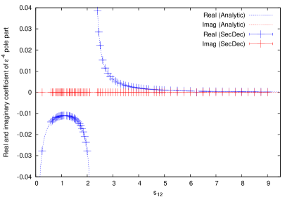
(a) leading pole

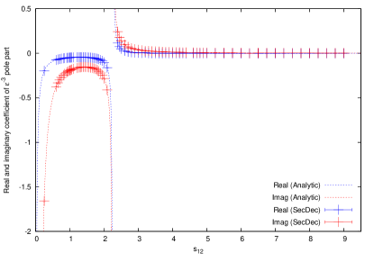
(b) subleading pole

Figure 5: Comparison of (a) the leading and (b) the subleading pole coefficients between the analytic result from [7] and the SecDec  result, for both real part (blue) and imaginary part (red). We vary $s_{12}$ and fix $s_{23}=-1.25,p_{3}^{2}=p_{4}^{2}=m^{2}=1$.

For two selected phase space points, we also compared the full result for all Laurent coefficients including the finite part to the result obtained analytically [34] and find agreement within the numerical integration errors. Our numerical results for the remaining pole coefficients and the finite part of the diagram ggtt2 are shown in Figs. 6 and 7.

The timings for the leading and subleading pole coefficients of the diagram ggtt2 are ranging between fractions of a second and about 20 seconds. The coefficients of the $1/\epsilon^{2}$ pole take between 13 and 300 seconds, while the coefficients of the $1/\epsilon$ pole take between 75 and 3000 seconds, depending on their distance to thresholds. For the finite part, the integration times range from 250 seconds to 4000 seconds. For all Laurent coefficients, a relative accuracy of $5\times 10^{-3}$ has been required, which has not always been reached for the $1/\epsilon$ and $\epsilon^{0}$ coefficients. It also should be noted that the timings for points close to threshold depend rather sensitively on the settings for the Monte Carlo integration parameters.

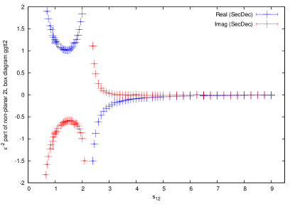
(a) $1/\epsilon^{2}$ pole

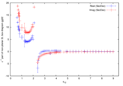
(b) $1/\epsilon$ pole

Figure 6: Results for (a) the $1/\epsilon^{2}$ and (b) the $1/\epsilon$ coefficients of the integral ggtt2. The kinematics are the same as in Fig. 5.

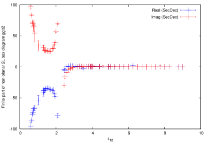
(a) finite part, including threshold

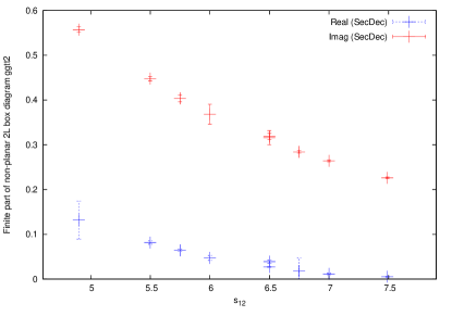
(b) finite part, beyond threshold

Figure 7: Results for the finite part of the scalar integral ggtt2, (a) for a larger kinematic range, (b) zoom into a region further away from threshold. The kinematics are the same as in Fig. 5. The vertical bars denote the numerical integration errors.

4.3 Massive tensor two-loop two-point functions

Here we show that the option to evaluate integrals with a non-trivial numerator can also be applied to calculate two-loop two-point functions involving different mass scales, without the need for a reduction to master integrals. This fact can be used for instance to calculate two-loop corrections to mass parameters in a straightforward way. As an example we pick the diagram shown in Fig. 8.

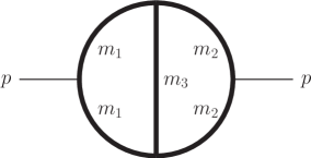
Figure 8: Two-loop bubble diagram with different masses

We calculate scalar integrals and rank three tensor integrals, for two cases, one where $m_{3}$ is zero, and one where $m_{3}$ is nonzero. The tensor integral is given by

$$\mathcal{G}_{B} =\left(\frac{1}{\mathrm{i}\pi^{\frac{\mathrm{D}}{2}}}\right)^{2}\int\frac{\mathrm{d^{D}}k_{1}\,\mathrm{d^{D}}k_{2}\,\,(k_{1}\cdot k_{2})\,(k_{1}\cdot p_{1})}{D_{1}\ldots D_{5}}\;\,;\,$$ (19)

$$D_{1}=k_{1}^{2}-m_{1}^{2},D_{2}=(k_{1}+p_{1})^{2}-m_{1}^{2},D_{3}=(k_{1}-k_{2})^{2}-m_{3}^{2},$$

$$D_{4}=(k_{2}+p_{1})^{2}-m_{2}^{2},D_{5}=k_{2}^{2}-m_{2}^{2}\;.$$

The fact that this tensor integral is reducible does not play a role here, because our purpose is to demonstrate that reduction may become obsolete considering the short integration times for the tensors. Results for the scalar and tensor integrals with $m_{3}=0$ are shown in Fig. 9, while results for $m_{3}^{2}=3$ are shown in Fig. 10.

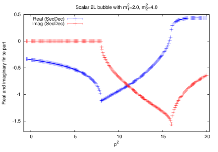
(a) scalar integral

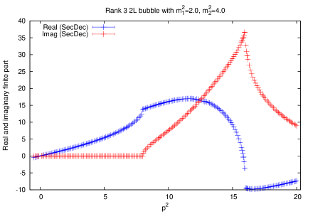
(b) rank 3 tensor integral

Figure 9: Results for real (blue) and imaginary (red) parts of the rank 3 two-loop bubble diagram shown in Fig. 8, (a) scalar case, (b) with numerator $(k_{1}\cdot k_{2})\,(k_{1}\cdot p_{1})$. The masses are $m_{1}^{2}=2,m_{2}^{2}=4,m_{3}=0$.

The timings for the massive two-point integrals are shown in Figs. 11 (a) and (b), for $m_{3}^{2}=0$ and $m_{3}^{2}=3$, respectively. The timings were obtained on computers with Intel i7 processors and 8 cores. In both cases, a relative accuracy of 0.1% was required for the Monte Carlo integration. In Fig. 11 (a), an absolute desired accuracy of $10^{-3}$ was set, in Fig. 11 (b) an absolute accuracy of $10^{-6}$. Fig. 11 shows that for values of $p^{2}$ above the mass threshold at $p^{2}=4m_{2}^{2}$, the timings for the contracted rank three tensor integrals do not differ much from the ones for the scalar integrals. In the region below threshold, the timings are higher because the imaginary part is zero, and a vanishing function is difficult to integrate numerically. As the relative error to a zero value is always infinite, the numerical integrator in this case tries to reach the absolute accuracy goal. If in addition to the vanishing imaginary part the real part is also close to zero, the integration times are highest, as can be seen from Figs. 10 and 11 (b). To avoid artificially large timings in kinematic regions where the imaginary part is known to be zero, one could set contourdef=false for the kinematic points below threshold. This would have the effect that the imaginary part is not calculated at all, but set to zero from scratch, thereby reducing the integration time considerably. The minimal numerical integration time for a kinematic point above threshold in the case of the scalar two-loop bubble integrals is 0.03 secs for $m_{3}^{2}\not=0$ and 0.02 secs for $m_{3}^{2}=0$.

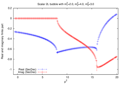
(a) scalar integral

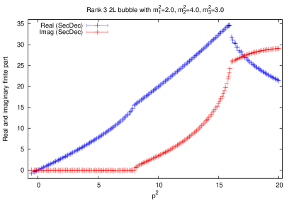
(b) rank 3 tensor integral

Figure 10: Results for the rank 3 two-loop bubble diagram with three non-vanishing masses, shown in Fig. 8, (a) scalar case, (b) tensor case with numerator $(k_{1}\cdot k_{2})\,(k_{1}\cdot p_{1})$. The masses are $m_{1}^{2}=2,m_{2}^{2}=4,m_{3}^{2}=3$.

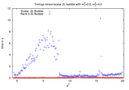
(a) $m_{3}=0$

(b) $m_{3}^{2}=3$

Figure 11: Comparison of evaluation times between the scalar and the rank three tensor integrals corresponding to a two-loop two-point function with 3 different masses. The red points are the evaluation times in seconds for the scalar integral at a given kinematic point, the timings for the rank 3 tensor integral are marked in blue.

5 Conclusions

We have presented numerical results for two massive non-planar seven propagator topologies, one entering the light fermionic two-loop correction to the $gg\to t\bar{t}$ channel, the other one entering the heavy fermionic correction to this channel. For the latter, no analytical result is available yet. Apart from the scalar master integral, we also give results for an irreducible tensor numerator of rank two for this diagram. Our numerical results have been obtained with the program SecDec2.1, which is publicly available at
http://secdec.hepforge.org. Compared to version 2.0 of SecDec, version 2.1 contains a number of new features, among them the possibility to evaluate tensor integrals with no principle limitation on the rank. The applicability of the tensor option to various types of integrals is further demonstrated by a number of results for two-loop two-point functions involving several different mass scales, where no analytical results exist. Another new feature is the option to apply the sector decomposition algorithm and subsequent contour deformation on user-defined functions which do not necessarily have the form of standard loop integrals. This new feature is used in combination with a novel type of analytic transformations, which can serve to reduce the number of functions to be integrated numerically. We believe that SecDec  version 2.1 brings us a major step forward in moving from the calculation of master integrals to the calculation of two-loop corrections for phenomenological applications.

A Appendix

A.1 Usage of the program

1. Change to the subdirectory loop or general. The setup in the loop directory should be used to calculate loop integrals and integrals with a similar structure. The option to use contour deformation is available for all functions processed within the loop directory. The setup in the general directory allows to evaluate more general parameter integrals, which can have endpoint singularities at zero and one, but does not offer contour deformation.

2. In the general directory, copy the files param.input and
   template.m to create your own parameter and template files
   myparamfile.input, mytemplatefile.m and edit them according to the function to be calculated. In the loop directory, edit the files
   paramloop.input and templateloop.m if you want to compute a Feynman loop integral in a fully automated way. If you would like to define a set of own functions rather than a standard loop integral, use the files paramuserdefined.input and templateuserdefined.m as a starting point.

3. Set the desired parameters in myparamfile.input and specify the integrand in mytemplatefile.m.

4. Execute the command ./launch -p myparamfile.input -t mytemplatefile.m in the shell. If you add the option -u in the loop directory, user defined functions are computed.
   If you omit the option -p myparamfile.input, the file param.input will be taken as default. Likewise, if you omit the option -t mytemplatefile.m, the file template.m will be taken as default. If your files myparamfile.input, mytemplatefile.m are in a different directory, say, myworkingdir, use the option -d myworkingdir, i.e. the full command then looks like ./launch -d myworkingdir -p myparamfile.input -t mytemplatefile.m, executed from the directory SecDec/loop or SecDec/general.

5. Collect the results. Depending on whether you have used a single machine or submitted the jobs to a cluster, the following actions will be performed:

   • If the calculations are done sequentially on a single machine, the results will be collected automatically (via the corresponding results*.pl called by launch). The output file will be displayed with your specified text editor.

   • If the jobs have been submitted to a cluster, when all jobs have finished, execute the command ./results.pl [-d myworkingdir -p myparamfile] in the general, and ./resultsloop.pl [-d myworkingdir -p myparamfile] or ./resultsuserdefined.pl [-d myworkingdir -p myparamfile] in the loop directory, respectively. This will create the files containing the final results in the graph subdirectory specified in the input file.

6. After the calculation and the collection of the results is completed, you can use the shell command ./launchclean[graph] to remove obsolete files.

A.2 Evaluation of user-defined functions in the loop directory

In the following, we will describe the input and syntax needed for the files
mytemplatefile.m and myparamfile.input when treating functions which are different from the standard Feynman parameter representation which – in the default setup – is derived automatically from the propagators or vertices of a multi-loop integral.

The file mytemplatefile.m should contain the following information:

• List of user-defined functions:
  The user-defined functions should be polynomial in the Feynman parameters. They can contain monomial factors of Feynman parameters with arbitrary exponents, functions of type $\mathcal{U}$ and $\mathcal{F}$ (i.e. polynomials in the Feynman parameters involving also kinematic invariants) with arbitrary exponents and a “numerator” with positive exponents only. An iterated sector decomposition is applied to $\mathcal{U}$ and $\mathcal{F}$ if the decomposition flag (see below) is set to B. In case the functions $\mathcal{U}$ and $\mathcal{F}$ contain thresholds, a deformation of the integration contour into the complex plane becomes necessary. The setup is such that the integration contour will be formed based on the function $\mathcal{F}$. The list of user-defined functions must be inserted into mytemplatefile.m using the following syntax
  functionlist={function_1,function_2,…,function_i,…};
  with
  function_i={# of function,{list of exponents},{{function $\mathcal{U}$, exponent of $\mathcal{U}$, decomposition flag},{function $\mathcal{F}$,exponent of $\mathcal{F}$,decomposition flag}}, numerator}.
  The # of function of each user-defined function is a label of the function by an integer, where the default is just sequential numbering. However, there is also the option to label a set of functions with the same integer. In this case the functions are decomposed individually, but will be combined after the decomposition. This leads to fewer or simpler integrand functions when symmetries are found within a sector. It should be noted however that only functions which share the same exponent for all functions of type $\mathcal{U}$ respectively $\mathcal{F}$ can be grouped together and therefore have the same function label.

  Each entry in the comma separated list of exponents corresponds to an exponent of a Feynman parameter occurring as a monomial in the Feynman integral. The decomposition flag should be A if no iterated sector decomposition is desired, and B if the function needs further decomposition. The numerator may contain several functions, with different non-negative exponents.

• Dimension, kinematic conditions:
  The space-time dimension should be specified in mytemplatefile.m via
  Dim=dimension. The default is Dim=$4-2\epsilon$.
  On-shell conditions can be specified in the list onshell={}.

• Computation of the exponents of $\mathcal{F}$ and $\mathcal{U}$ (optional):
  If the exponents of the functions $\mathcal{F}$ and $\mathcal{U}$ should be computed by the program according to the rules for standard multi-loop integrals, the user needs to specify the number of propagators and their powers in a list powerlist=Table[power,{i,#propagators}]; and the tensor rank of the diagram via rank=rank;  .
  Here, #propagators should correspond to the number of propagators of the original Feynman diagram, or, more general, to the number of integration variables plus one.

In addition to the changes made to mytemplatefile.m, it is possible to set a maximal number of Feynman parameters occurring in the user defined functions by initalizing feynpars=… in myparamfile.input. The default is the number of propagators $N$ subtracted by one.
A full example including detailed comments comes with the download of the program and can be found in /loop/templateuserdefined.m and
/loop/paramuserdefined.input.

A.3 Evaluation of tensor integrals

For the computation of tensor integrals, where the tensor is contracted with external momenta and/or loop momenta, the construction of the Feynman integral via topological cuts needs to be switched off, which corresponds to cutconstruct=0.
Regarding the user input, the only additional information needed is the numerator in mytemplatefile.m. Each scalar product of loop momenta contracted with either external momenta or other loop momenta should be given as an entry of a list:
numerator={prefactor,comma separated list of scalar products}. For example, a numerator of the form -$2\,k_{1}\cdot k_{2}$, where $k_{1}$ and $k_{2}$ are loop momenta, should be given as numerator={$-2$, $k1*k2$ }. A numerator of the form $2\,(k_{1}\cdot p_{1})(k_{1}\cdot k_{2})$, where $p_{1}$ is an external momentum, should be given as
numerator={2, $k1*p1$, $k1*k2$ }.

References

- [1] M. Czakon and A. Mitov, NNLO corrections to top pair production at hadron colliders: the quark-gluon reaction, JHEP 1301 (2013) 080, [arXiv:1210.6832].
- [2] M. Czakon and A. Mitov, NNLO corrections to top-pair production at hadron colliders: the all-fermionic scattering channels, JHEP 1212 (2012) 054, [arXiv:1207.0236].
- [3] P. Baernreuther, M. Czakon, and A. Mitov, Percent Level Precision Physics at the Tevatron: First Genuine NNLO QCD Corrections to , Phys.Rev.Lett. 109 (2012) 132001, [arXiv:1204.5201].
- [4] R. Bonciani, A. Ferroglia, T. Gehrmann, A. Manteuffel, and C. Studerus, Two-Loop Leading Color Corrections to Heavy-Quark Pair Production in the Gluon Fusion Channel, JHEP 1101 (2011) 102, [arXiv:1011.6661].
- [5] R. Bonciani, A. Ferroglia, T. Gehrmann, and C. Studerus, Two-Loop Planar Corrections to Heavy-Quark Pair Production in the Quark-Antiquark Channel, JHEP 0908 (2009) 067, [arXiv:0906.3671].
- [6] R. Bonciani, A. Ferroglia, T. Gehrmann, D. Maitre, and C. Studerus, Two-Loop Fermionic Corrections to Heavy-Quark Pair Production: The Quark-Antiquark Channel, JHEP 0807 (2008) 129, [arXiv:0806.2301].
- [7] A. von Manteuffel, “Talk given at the conference ACAT 2011, Uxbridge, London, September 2011.”
- [8] A. von Manteuffel and C. Studerus, Top quark pairs at two loops and Reduze 2, arXiv:1210.1436. To appear in the proceedings of the conference “Loops and Legs in Quantum Field Theory”, 2012.
- [9] G. Abelof, A. Gehrmann-De Ridder, and O. Dekkers, Antenna subtraction with massive fermions at NNLO: Double real initial-final configurations, JHEP 1212 (2012) 107, [arXiv:1210.5059].
- [10] G. Abelof and A. Gehrmann-De Ridder, Double real radiation corrections to production at the LHC: the channel, JHEP 1211 (2012) 074, [arXiv:1207.6546].
- [11] G. Abelof and A. Gehrmann-De Ridder, Double real radiation corrections to production at the LHC: the all-fermion processes, JHEP 1204 (2012) 076, [arXiv:1112.4736].
- [12] J. Korner, Z. Merebashvili, and M. Rogal, NNLO results for heavy quark pair production in quark-antiquark collisions: The One-loop squared contributions, Phys.Rev. D77 (2008) 094011, [arXiv:0802.0106].
- [13] M. Aliev, H. Lacker, U. Langenfeld, S. Moch, P. Uwer, et al., HATHOR: HAdronic Top and Heavy quarks crOss section calculatoR, Comput.Phys.Commun. 182 (2011) 1034–1046, [arXiv:1007.1327].
- [14] M. Czakon and A. Mitov, Precision top pair production at hadron colliders, arXiv:1303.0693.
- [15] S. Moch, P. Uwer, and A. Vogt, On top-pair hadro-production at next-to-next-to-leading order, Phys.Lett. B714 (2012) 48–54, [arXiv:1203.6282].
- [16] M. Cacciari, M. Czakon, M. Mangano, A. Mitov, and P. Nason, Top-pair production at hadron colliders with next-to-next-to-leading logarithmic soft-gluon resummation, Phys.Lett. B710 (2012) 612–622, [arXiv:1111.5869].
- [17] M. Czakon and A. Mitov, Top++: A Program for the Calculation of the Top-Pair Cross-Section at Hadron Colliders, arXiv:1112.5675.
- [18] M. Beneke, P. Falgari, S. Klein, and C. Schwinn, Hadronic top-quark pair production with NNLL threshold resummation, Nucl.Phys. B855 (2012) 695–741, [arXiv:1109.1536].
- [19] M. Beneke, P. Falgari, S. Klein, J. Piclum, C. Schwinn, et al., Inclusive Top-Pair Production Phenomenology with TOPIXS, JHEP 1207 (2012) 194, [arXiv:1206.2454].
- [20] V. Ahrens, A. Ferroglia, M. Neubert, B. D. Pecjak, and L. L. Yang, Precision predictions for the t+t(bar) production cross section at hadron colliders, Phys.Lett. B703 (2011) 135–141, [arXiv:1105.5824].
- [21] N. Kidonakis, Next-to-next-to-leading soft-gluon corrections for the top quark cross section and transverse momentum distribution, Phys.Rev. D82 (2010) 114030, [arXiv:1009.4935].
- [22] M. Czakon, Tops from Light Quarks: Full Mass Dependence at Two-Loops in QCD, Phys.Lett. B664 (2008) 307–314, [arXiv:0803.1400].
- [23] M. Czakon, A. Mitov, and S. Moch, Heavy-quark production in massless quark scattering at two loops in QCD, Phys.Lett. B651 (2007) 147–159, [arXiv:0705.1975].
- [24] M. Czakon, A. Mitov, and S. Moch, Heavy-quark production in gluon fusion at two loops in QCD, Nucl.Phys. B798 (2008) 210–250, [arXiv:0707.4139].
- [25] J. Carter and G. Heinrich, SecDec: A general program for sector decomposition, Comput.Phys.Commun. 182 (2011) 1566–1581, [arXiv:1011.5493].
- [26] S. Borowka, J. Carter, and G. Heinrich, Numerical Evaluation of Multi-Loop Integrals for Arbitrary Kinematics with SecDec 2.0, Comput.Phys.Commun. 184 (2013) 396–408, [arXiv:1204.4152].
- [27] S. Borowka and G. Heinrich, Numerical evaluation of massive multi-loop integrals with SecDec, arXiv:1209.6345. To appear in the proceedings of the conference “Loops and Legs in Quantum Field Theory”, 2012.
- [28] T. Binoth and G. Heinrich, An automatized algorithm to compute infrared divergent multi-loop integrals, Nucl. Phys. B585 (2000) 741–759, [hep-ph/0004013].
- [29] G. Heinrich, Sector Decomposition, Int. J. Mod. Phys. A23 (2008) 1457–1486, [arXiv:0803.4177].
- [30] T. Binoth and G. Heinrich, Numerical evaluation of multi-loop integrals by sector decomposition, Nucl. Phys. B680 (2004) 375–388, [hep-ph/0305234].
- [31] C. Anastasiou, F. Herzog, and A. Lazopoulos, On the factorization of overlapping singularities at NNLO, JHEP 1103 (2011) 038, [arXiv:1011.4867].
- [32] T. Hahn, CUBA: A library for multidimensional numerical integration, Comput. Phys. Commun. 168 (2005) 78–95, [hep-ph/0404043].
- [33] S. Agrawal, T. Hahn, and E. Mirabella, FormCalc 7, arXiv:1112.0124.
- [34] A. von Manteuffel, “private communication.”