Interference and transport properties of conductions electrons on the surface of a topological insulator

Abstract

The surface conductivity for conduction electrons with a fixed chirality in a topological insulator with impurities scattering is considered. The surface excitations are described by the Weyl Hamiltonian. For a finite chemical potential one projects out the hole band and one obtains a single electronic band with a fixed chirality. One obtains a model of spinless electrons which experience a half vortex when they return to the origin. As a result the conductivity is equivalent to a spinless problem with correlated noise which gives rise to anti-localization. We compute conductivity as a function of frequency and compare our results with the $Raman$ shift measurement for $Bi_{2}Se_{3}$.

I. Introduction

Topological insulators ($TI$) are time reversal invariant systems which obey Kramers theorem Volkov ; Kane ; Zhang ; David . Toplogical insulators are characterized by the surface excitations and are described by the $Weyl$ Hamiltonian. $Bi_{2}Se_{3}$ is such a material which is described by the $Weyl$ equation with a single Dirac cone which lies below the chemical potential $\mu$ and the bulk gap. Due to time reversal symmetry the backscattering is suppressed in agreement with scanning tunneling microscopy (STM) experiment and theory Balatsky . Conductivity results are less conclusive, due to the presence of the $3D$ bulk gap Culcer or the insulating gap observed in thin layers of $TI$.

The charge current for the Weyl equation is identified with the spin half operator. As a result the charge current and the spin current are related to each other Raghu . In the presence of impurities, elastic scattering conserves energy but not quasi-momentum giving rise to a finite conductivity.

Transport properties have been calculated building on the relation with the spin-orbit model, which belongs to the symplectic ensemble Hikami and therefore quantum interference gives rise to anti-localization. These results have been confirmed by Ando and Hankiewicz ; Stern ; Shen ; Garate .

The purpose of this work is to compute the surface conductivity for the Weyl Hamiltonian with a finite chemical potential $\mu$. The surface Hamiltonian for a single Dirac cone and a finite chemical potential has been obtained in ref. Raghu and can be described by the Weyl Hamiltonian Maggiore with a Fermi velocity $v\approx 5\times 10^{6}$ $\frac{m}{sec}$ and a chemical potential $\mu\approx 0.1$ eV. The Weyl Hamiltonian is characterized by opposite chirality for electrons and holes. For a large chemical potential we can replace the Weyl Hamiltonian by a single electronic band with a fixed chirality. The model resembles a spinless model in two dimensions, therefore the presence of elastic scattering might give rise to localization. The backscattering potential for a single scattering is zero but multi-scattering are allowed. Therefore we might expect localization . Consequently, a particle can backscatter after two scatterings allowing a decrease in the conductivity. The difference between the one band spinless electrons and our case arising from the fact that the conduction electrons are obtained after a projection of the chiral spinors of the Weyl spin half fermions. The effect of the projection modifies the random scattering matrix elements but preserve the property of spin half spinor introducing correlations which are determined by the momentum difference between the incoming and outgoing electrons. In order to determine the quantum corrections we compute the quantum return probability $P_{qm}$ given by the interference between a closed path and the time reversed path. Due to the projection which preserve the spin half vortex at $\vec{k}=0$ the quantum return probability $P_{qm}$ vanishes. Using these results we compute the conductivity using the method employed for spinless electrons. The impurity scattering affects the charge and gives rise to the maximal crossed corrections Rammer . We find that the charge is enhanced giving rise to an enhanced transport life time. Due to the angle dependent scattering the maximal crossed diagrams change sign and give rise to anti-localization. This effect result is similar with the results obtained by Ando in graphene with a zero chemical potential.

The plan of this paper is as follows. In Sec. $II$ we introduce the Weyl model. We construct the quantized particle and anti-particle bands imposing the time reversal symmetry. Due to the singularity at $\vec{k}=0$ the unperturbed spinor must be obey the the Pfaffian properties Kane . In Sec. $III$ we consider the model for a single conduction band .In Sec. $IV$ we compute the quantum return probability for the one band model. In Sec. $V$ we construct the Green’s functions Abrikosov for the conduction electrons. We compute the $ladder$ and $maximal$ $crossed$ diagram . In Sec. $VI$ we compute the static and frequency dependent conductivity. In Sec. $VII$ we discuss our results and propose that a good confirmation of the surface conductivity can be obtained from Raman scattering Conder .In Sec. $VIII$ we present our conclusions.

II. The Weyl model

The surface state Hamiltonian for a topological insulator of the $Bi_{2}Se_{3}$ family materials is given by the Weyl model Raghu . The presence of a random potential and an electromagnetic field modify the Weyl model in the following way:

$$S=\int\,dt\left[\int\,d^{2}r\Psi^{\dagger}(\vec{r},t)(i\partial_{t}-eA_{0}(\vec{r},t))\Psi(\vec{r},t)-H\right],$$

$$H=\hbar v\int\,d^{2}r\Psi^{\dagger}(\vec{r})\left[\sigma^{1}(-i\partial_{2}-\frac{e}{\hbar}A_{2}(\vec{r},t))-\sigma^{2}(-i\partial_{1}-\frac{e}{\hbar}A_{1}(\vec{r},t))+U_{sc}(\vec{r})\right]\Psi(\vec{r}),$$

where $\vec{A}(t)=\frac{\vec{E}(\Omega)}{i\Omega}e^{-i\Omega t}$ is the external vector potential, $A_{0}(\vec{r},t)$ is the external scalar potential and $U_{sc}(\vec{r})$ is the random potential controlled by the white noise correlation function $\langle\langle U_{sc}(\vec{k})U_{sc}(\vec{k}^{\prime})\rangle\rangle=D_{sc}\delta^{2}[\vec{k}+\vec{k}^{\prime}]$. The unperturbed Weyl Hamiltonian in the first quantized form is given by $h[\vec{k}]=-\sigma^{2}k_{1}+\sigma^{1}k_{2}$. Here $h[\vec{k}]$ is time reversal invariant and obeys the transformation relation $\vartheta^{-1}h[\vec{k}]\vartheta=h[-\vec{k}]$, where $\vartheta=i\sigma^{2}K$ is the time reversal operator and $K$ is the conjugation operator. The eigenstates form a Kramers degenerate pair with the property $\vartheta^{2}=-1$. At the point $\vec{k}=0$ the eigenvectors $|u^{(+)}(\vec{k})\rangle$, $|u^{(-)}(\vec{k})\rangle$ are degenerate and we need to choose a representation where the eigenvectors are orthogonal to each other. In order to regularize the problem we will replace the Hamiltonian $h[\vec{k}]=-\sigma^{2}k_{1}+\sigma^{1}k_{2}$ by:

$$h[\vec{k}]=-\sigma^{2}k_{1}+\sigma^{1}k_{2}+\sigma^{3}\eta M(\vec{k}),\hskip 7.22743pt\eta\rightarrow 0.$$ (2)

We introduce the function $\theta[M(\vec{k})]$ which is one for $M(\vec{k})\geq 0$ and zero otherwise. We solve the eigenvalue equation in the presence of the mass term $M(\vec{k})$ . For the region $\theta[M(\vec{k})]=1$ find that that the eigenvector $|u_{1}(\vec{k})\rangle$ corresponds to the positive eigenvalues and eigenvector $|u_{2}(\vec{k})\rangle$ to the negative eigenvalues . For the region $\theta[-M(\vec{k})]=1$ the eigenvector $|u_{2}(\vec{k})\rangle$ corresponds to positive eigenvalues and $|u_{1}(\vec{k})\rangle$ correspond to the negative eigenvalues. Using a mass term which preserve time reversal symmetry $M(\vec{k})=-M(-\vec{k})$, we guarantee that the eigenvectors at the point $\vec{k}=0$ are orthogonal to each other and obey Krammers theorem. We will consider the limit $\eta\rightarrow 0$ and neglect the energy corrections but we will consider the topological effects caused by the mass term $M(\vec{k})$ which preserve the time reversal symmetry $\vartheta^{2}=-1$. We note that for the $wrapping$ case, the mass $M(\vec{k})=(k_{1}+ik_{2})^{3}+(k_{1}-ik_{2})^{3}=2k_{1}(k^{2}_{1}-3k^{2}_{2})$ provide a natural regularization for the eigenvectors at $\vec{k}=0$ . The eigenvectors $|u_{1}(\vec{k})\rangle$ and $|u_{2}(\vec{k})\rangle$ are given in terms of the multivalued phase phase $\chi(\vec{k})$, $\tan(\chi(\vec{k})=\frac{k_{2}}{k_{x}}$ :

$$|u_{1}(\vec{k})\rangle=\frac{1}{2}\Big{[}|\vec{k}\rangle\otimes[1,-ie^{i\chi(\vec{k})}]^{T}\Big{]},\hskip 14.45377pt|u_{2}(\vec{k})\rangle=\frac{1}{2}\Big{[}|\vec{k}\rangle\otimes[ie^{-i\chi(\vec{k})},1]^{T}\Big{]},$$ (3)

The phase $\chi(\vec{k})$ obey the property $\chi(-\vec{k})=\pi+\chi(\vec{k})$. $|u_{1}(\vec{k})\rangle$ and $|u_{2}(\vec{k})\rangle$ form a Kramers pair. Due to the time reversal symmetry the two eigenvectors are related through the Pfaffian matrix, $W_{1,2}(\vec{k})=\langle u_{1}(\vec{k})|\vartheta|u_{2}(\vec{k})\rangle$ with $|u_{1}(-\vec{k})\rangle=W^{*}_{1,2}(\vec{k})\vartheta u_{2}(\vec{k})\rangle$ and $|u_{2}(-\vec{k})\rangle=W^{*}_{2,1}(\vec{k})\vartheta|u_{1}(\vec{k})\rangle$. The spinors $|u_{1}(\vec{k})\rangle$ and $|u_{2}(\vec{k})\rangle$ will be used to construct the eigenvector $|u^{(+)}(\vec{k})\rangle$ for particles and $|u^{(-)}(\vec{k})\rangle$ for antiparticles for the entire Brillouin zone.

$$|u^{(-)}(\vec{k})\rangle=\theta[M(\vec{k})]|u_{2}(\vec{k})\rangle+\theta[M(-\vec{k})]|u_{1}(\vec{k}\rangle,$$

$$|u^{(+)}(\vec{k})\rangle=\theta[M(\vec{k})]|u_{1}(\vec{k})\rangle+\theta[M(-\vec{k})]|u_{2}(\vec{k})\rangle.$$

The eigenvector $|u^{(+)}(\vec{k})\rangle$ corresponds to the eigenvalue $E_{p}=E_{+}=\hbar v|\vec{k}|$ (for particles) and $|u^{(-)}(\vec{k})\rangle$ corresponds to the eigenvalue $E_{a}=E_{-}=-\hbar v|\vec{k}|$ (for anti-particle). The eigenspinors chage the sign under a full rotation of $2\pi$. In two dimensions a full rotation of $2\pi$ is equivalent to two consecutive inversions. We introduce the inversion operator $P$, $P|u^{(+)}(\vec{k})\rangle=|u^{(+)}(-\vec{k})\rangle$, $P|u^{(-)}(\vec{k})\rangle=|u^{(-)}(-\vec{k})\rangle$ and find that $P^{2}=-1$:

$$P^{2}e^{\frac{\pm i}{2}\chi(\vec{k})}=Pe^{\frac{\pm i}{2}\chi(-\vec{k})}=Pe^{\frac{\pm i}{2}(\chi(\vec{k})+\pi)}=e^{\frac{\pm i}{2}(\chi(-\vec{k})+\pi)}=e^{\frac{\pm i}{2}(\chi(\vec{k})+\pi+\pi)}=e^{i\pi}e^{\frac{\pm i}{2}\chi(\vec{k})}=-e^{\frac{\pm i}{2}\chi(\vec{k})}$$

$$P^{2}|u^{(+)}(\vec{k})\rangle=-|u^{(+)}(\vec{k})\rangle;P^{2}|u^{(-)}(\vec{k})\rangle=-|u^{(-)}(\vec{k})\rangle$$

This shows that the two eigenspinors $|u^{(\pm)}(\vec{k})\rangle$ behave like a spin half fermion under rotations.

We will include the Fermi velocity $v$ to describe the physical energy spectrum. In order to incorporate the velocity in the Hamiltonian we multiply the spinor operator by $\sqrt{v}$. The spinor operator $\Psi(\vec{r})$ is decomposed into the eigenmodes of the unperturbed Weyl Hamiltonian.

$$\Psi(\vec{r})=\sqrt{v}\sum_{\vec{k}}e^{i\vec{k}\cdot\vec{r}}[C(\vec{k})u^{(+)}(\vec{k})+B^{\dagger}(-\vec{k})u^{(-)}(-\vec{k})]\equiv\sqrt{v}\sum_{\vec{k}}e^{i\vec{k}\cdot\vec{r}}\Psi(\vec{k}).$$ (6)

We choose that particle operators $C(\vec{k})$, $C^{\dagger}(\vec{k})$ and the anti-particle operators $B(\vec{k})$, $B^{\dagger}(\vec{k})$ should obey anti-commutation relations:

$$[C(\vec{k}),C^{\dagger}(\vec{k^{\prime}})]_{+}=[B(\vec{k}),B^{\dagger}(\vec{k^{\prime}})]_{+}=\delta^{(2)}[\vec{k}-\vec{k^{\prime}}],\hskip 7.22743pt[C(\vec{k}),C(\vec{k^{\prime}})]_{+}=[B(\vec{k}),B(\vec{k^{\prime}})]_{+}=0.$$ (7)

The spinor projection $\Psi_{\sigma}(\vec{r})\equiv\langle\Psi(\vec{r})|\sigma\rangle$ obeys the modified anti-commutation relations:

$$.[\Psi_{\sigma}(\vec{r}),\Psi^{\dagger}_{\sigma^{\prime}}(\vec{r^{\prime}})]_{+}=v\delta_{\sigma,\sigma^{\prime}}\delta^{(2)}(\vec{r},\vec{r^{\prime}}),\hskip 7.22743pt[\Psi_{\sigma}(\vec{r}),\Psi_{\sigma^{\prime}}(\vec{r^{\prime}})]_{+}=0,$$ (8)

For a a chemical potential $\mu=\hbar vk_{F}>0$ ($k_{F}$ is the Fermi momentum) we introduce the notation $|\mu>$ for the ground state. The particle operator $C(\vec{k})$ and the anti-particle operator $B(\vec{k})$ annihilate the ground state, $C(\vec{k})|\mu\rangle=0$ for $E(\vec{k})>\mu>0$. We will consider a situation where the chemical potential $\mu$ measured from the Dirac point has the typical value of $0.01$ eV with a Fermi velocity $v$ of $5\times 10^{5}$ $\frac{m}{sec}$. Using the eigenspinors given in eq. $(4)$ we find that the Hamiltonian in the present of the scattering potential $U_{sc}(\vec{k}-\vec{p})$ is equivalent to two coupled bands.

$$H_{0}=\sum_{\vec{k}}[(\hbar v|\vec{k}|-\mu)C^{\dagger}(\vec{k})C(\vec{k})+(\hbar v|\vec{k}|+\mu)B^{\dagger}(-\vec{k})B(-\vec{k})],$$

$$H_{D}=\sum_{\vec{k}}\sum_{\vec{p}}vU_{sc}(\vec{k}-\vec{p})\Big{[}V^{(p,p)}(\vec{k},\vec{p})C^{\dagger}(\vec{k})C(\vec{p})+V^{(a,a)}(-\vec{k},-\vec{p})B(-\vec{k})B^{\dagger}(-\vec{p})$$

$$+V^{(p,a)}(\vec{k},-\vec{p})C^{\dagger}(\vec{k})B^{\dagger}(-\vec{p})+V^{(a,p)}(-\vec{k},\vec{p})B(-\vec{k})C(\vec{p})\Big{]},$$

where $H_{0}$ is the unperturbed Hamiltonian and $H_{D}$ represent the effect of the impurity scattering. The spinors structure gives rise to vertex functions for the coupling to the random potential in momentum space. The vertex functions are given in terms of the particle and anti-particle matrix elements ($p$ stands for particles and $a$ stands for antiparticles):

$$V^{(p,p)}(\vec{k},\vec{p})=\langle u^{(+)}(\vec{k})|u^{(+)}(\vec{p})\rangle,~{}~{}V^{(a,a)}(-\vec{k},-\vec{p})=\langle u^{(-)}(-\vec{k}))|u^{(-)}(-\vec{p})\rangle,$$

$$V^{(p,a)}(\vec{k},-\vec{p})=\langle u^{(+)}(\vec{k})|u^{(-)}(-\vec{p})\rangle,~{}~{}V^{(a,p)}(-\vec{k},\vec{p})=\langle u^{(-)}(-\vec{k})|u^{(+)}(\vec{p})\rangle.$$

From Eq. $(1)$ we obtain the external coupling of the electrons to the electromagnetic field $\vec{A}(\vec{r},t)$:

$$H^{ext}(t)=\int\,d^{2}r[\hat{J}_{1}(\vec{r},t)A_{1}(\vec{r},t)+\hat{J}_{2}(\vec{r},t)A_{2}(\vec{r},t)].$$ (11)

From Eq. ($1$) we also find that the currents are given by: $\hat{J}_{1}(\vec{r},t)\equiv(-e)v\Psi^{\dagger}(\vec{r})\sigma^{2}\Psi(\vec{r})$, $\hat{J}_{2}(\vec{r},t)\equiv(-e)v\Psi^{\dagger}(\vec{r})(-\sigma^{1})\Psi(\vec{r}).$

Using the linear response theory Doniach for the current-current correlation function in the presence of an external vector potential $A_{1}(t)=\frac{E_{1}}{i\Omega}e^{-i\Omega t}$ we compute the interband absorbtion. We find that the optical conductivity in the limit of weak disorder and frequencies $\Omega>2\mu$ is given by the universal relation $\sigma(\Omega>2\mu)=\frac{e^{2}\pi}{8h}$.

For a finite chemical potential $\mu$ we integrate the anti-particle band $H^{(a)}$:

$$H^{(a)}=\sum_{\vec{k}}(\hbar v|\vec{k}|+2\mu)B^{\dagger}(-\vec{k})B(-\vec{k})+\sum_{\vec{k}}\sum_{\vec{p}}vU_{sc}(\vec{k}-\vec{p})\Big{[}V^{(a,a)}(-\vec{k},-\vec{p})B(-\vec{k})B^{\dagger}(-\vec{p})$$

$$+V^{(p,a)}(\vec{k},-\vec{p})C^{\dagger}(\vec{k})B^{\dagger}(-\vec{p})+V^{(a,p)}(-\vec{k},\vec{p})B(-\vec{k})C(\vec{p})\Big{]}.$$

We perform the integration in the limit where white noise fluctuations are negligible in comparison with the chemical potential $\sqrt{D_{sc}}<\mu$. Under this condition the anti-particles can be integrated out. As a result the particle Hamiltonian is modified by the induced term $\delta H^{ind.}$ which can be understood as shift of the chemical potential.

$$\delta H^{ind.}=-\int\frac{d^{2}k}{2\pi}\int\frac{d^{2}q}{2\pi}\int\frac{d\omega}{2\pi}C^{\dagger}(\vec{k},\omega)$$

$$\left[\int\frac{d^{2}p}{2\pi}V^{(p,a)}(\vec{k},\vec{p})\frac{vU_{sc}(\vec{k}-\vec{p})U_{sc}(\vec{p}-\vec{k}+\vec{q})v}{[(E(\vec{k})+\Sigma(\vec{k},\omega;p))-(E(\vec{p})+\Sigma(\vec{p},\omega;a))-2\mu]}V^{(a,p)}(-\vec{p},\vec{k}-\vec{q})\right]C(\vec{k}-\vec{q},\omega).$$

Here $\Sigma(\vec{k},\omega;a)$ is the anti-particle self-energy induced by the disorder. When the chemical potential $\mu$ obeys the condition $|(E(\vec{k})+\Sigma(\vec{k},\omega;a))-(E(\vec{p})+\Sigma(\vec{p},\omega;a))-2\mu|\leq 2\mu$ we can perform the momentum $p$ integration which allows the replacement of $U_{sc}(\vec{k}-\vec{p})U_{sc}(\vec{p}-\vec{k}+\vec{q})$ with $\langle\langle U_{sc}(\vec{k}-\vec{p})U_{sc}(\vec{p}-\vec{k}+\vec{q})\rangle\rangle=D_{sc}\delta^{2}[\vec{q}]$. Consequently, the effective one-band Hamiltonian will have a new chemical potential $\mu\rightarrow\mu-\frac{D_{sc}v^{2}}{2\mu}$. Therefore for chemical potential $\mu$ which satisfies $\mu>\frac{D_{sc}}{2}$ the one-band approximation is justified.

III. The single band model

As a result of the discussion in the previous chapter we conclude that for a finite chemical potential the surface of the $TI$ can be described by a single band with a correlated potential.

$$H^{(c)}=\sum_{\vec{k}}(\hbar v|\vec{k}|-\mu)C^{\dagger}(\vec{k})C(\vec{k})+\sum_{\vec{k}}\sum_{\vec{p}}vU_{sc}(\vec{k}-\vec{p})V^{(p,p)}(\vec{k},\vec{p})C^{\dagger}(\vec{k})C(\vec{p})$$ (14)

Where $V^{(p,p)}(\vec{k},\vec{p})\equiv\langle u^{(+)}(\vec{k})|u^{(+)}(\vec{p})\rangle$ is evaluated with the help of explicit form of eigenspinors given in equation $(4)$. We introduce new operators $\hat{C}^{\dagger}(\vec{k})$ and $\hat{C}(\vec{k})$:

$$\hat{C}^{\dagger}(\vec{k})=C^{\dagger}(\vec{k})\Big{[}e^{\frac{i}{2}\chi(\vec{k})}\theta[M(\vec{k})]+e^{\frac{-i}{2}\chi(\vec{k})}\theta[-M(\vec{k})]\Big{]}$$

$$\hat{C}(\vec{k})=\Big{[}e^{\frac{-i}{2}\chi(\vec{k})}\theta[M(\vec{k})]+e^{\frac{i}{2}\chi(\vec{k})}\theta[-M(\vec{k})]\Big{]}C(\vec{k})$$

As a result we can express the Hamiltonian in eq. $(14)$ in the following way:

$$H^{(c)}=\sum_{\vec{k}}(\hbar v|\vec{k}|-\mu)\hat{C}^{\dagger}(\vec{k})\hat{C}(\vec{k})+\sum_{\vec{k}}\sum_{\vec{p}}v\hat{C}^{\dagger}(\vec{k})\Gamma_{\|}(\vec{k},\vec{p})\hat{C}(\vec{p})$$ (16)

In eq. ($16$) $\Gamma_{\|}(\vec{k},\vec{p})$ represents the scattering matrix.

$$\Gamma_{\|}(\vec{k},\vec{p})\equiv U_{sc}(\vec{k}-\vec{p})\hat{\Gamma}_{\|}(\vec{k},\vec{p});\hskip 7.22743pt\hat{\Gamma}_{\|}(\vec{k},\vec{p})=\cos[\frac{1}{2}(\chi(\vec{k})-\chi(\vec{p}))]$$ (17)

The angle $\chi(\vec{p})$ acts as a half vortex, when the momentum is reversed the angle $\chi(\vec{p})$ increases by $\pi$, $\chi(-\vec{p})=\chi(\vec{p})+\pi$. As a result we obtain: $\hat{\Gamma}_{\|}(\vec{k},-\vec{p})=\cos[\frac{1}{2}(\chi(\vec{k})-\chi(-\vec{p}))]=\cos[\frac{1}{2}(\chi(\vec{k})-\chi(\vec{p}))-\frac{\pi}{2}]=\sin[\frac{1}{2}(\chi(\vec{k})-\chi(\vec{p}))]$

For the backscattering direction $\vec{p}=-\vec{k}$ we find that the single particle scattering vanishes $\hat{\Gamma}_{\|}(\vec{k},-\vec{k})=0$.

Next we consider the coupling of the external vector potential to the conduction band only:

$$H^{ext}(t)=\int\ d^{2}r[J_{1}(\vec{r},t)A_{1}(\vec{r},t)+J_{2}(\vec{r},t)A_{2}(\vec{r},t)]=(-ev)\int\frac{d^{2}k}{(2\pi)^{2}}\int\frac{d^{2}p}{(2\pi)^{2}}$$

$$C^{\dagger}(\vec{k},t)C(\vec{p},t)[\langle u^{(+)}(\vec{k})|-\sigma^{2}|u^{(+)}(\vec{p})\rangle A_{1}(-(\vec{k}-\vec{p}),t)+\langle u^{(+)}(\vec{k})|\sigma^{1}|u^{(+)}(\vec{p})\rangle A_{2}(-(\vec{k}-\vec{p}),t)]$$

$$=(-ev)\int\frac{d^{2}k}{(2\pi)^{2}}\int\frac{d^{2}p}{(2\pi)^{2}}\hat{C}^{\dagger}(\vec{k},t)\hat{C}(\vec{p},t)\Big{[}W_{1}(\vec{k},\vec{p})A_{1}(-(\vec{k}-\vec{p}),t)+W_{2}(\vec{k},\vec{p})A_{2}(-(\vec{k}-\vec{p}),t)\Big{]},$$

where the vertex functions are given by:

$$W_{1}(\vec{k},\vec{p})=\cos[\frac{1}{2}(\chi(\vec{k})+\chi(\vec{p}))];\hskip 7.22743ptW_{2}(\vec{k},\vec{p})=-\sin[\frac{1}{2}(\chi(\vec{k})+\chi(\vec{p}))].$$ (19)

Using the definition of the current operator $J_{1}(\vec{q},t)=(-ev)\int\frac{d^{2}k}{(2\pi)^{2}}\int\frac{d^{2}p}{(2\pi)^{2}}W_{1}(\vec{k},\vec{p})\hat{C}^{\dagger}(\vec{k},t)\hat{C}(\vec{p},t)\delta^{2}[\vec{k}-\vec{p}-\vec{q}]$ we obtain from the linear response theory the induced current $\delta\langle J_{1}(\vec{q},t)\rangle=\int_{-\infty}^{\infty}dt_{1}R_{1,1}(\vec{q},t-t_{1})A_{1}(-\vec{q},t_{1})$ with the correlation function $R_{1,1}(\vec{q},t-t_{1})$ given by Doniach :

$$R_{1,1}(\vec{q},t-t_{1})=-\frac{i}{\hbar}\theta[t-t_{1}]\langle\Big{[}J_{1}(\vec{q},t),J_{1}(-\vec{q},t_{1})\Big{]}\rangle.$$ (20)

We perform the Fourier transform of $R_{1,1}(\vec{q},t-t_{1})$ with respect the frequency $\Omega$ and find that the conductivity is given by $\sigma(\vec{q}=0,\Omega)\equiv\frac{R_{1,1}(\vec{q}=0,\Omega)}{i\Omega}=\sigma(\Omega)$.

IV. Interference effects and the consequence for the conductivity

The quantum conductivity is controlled by the multiple scattering process of closed paths. The interference between a closed path and the time reversed paths allows to define the quantum return probability $P_{qm}$. If we denote by $\mathscr{T}$ the amplitude for a particle to return to the starting point and $T\mathscr{T}$ the time reversed amplitude, the quantum return probability $P_{qm}$ is given by $P_{qm}=(\mathscr{T}+T\mathscr{T})(\mathscr{T}+T\mathscr{T})^{*}$ ($T$is the time reversal operator). For time reversal invariant systems the quantum return probability is $P_{qm}=4(\mathscr{T})(\mathscr{T})^{*}$ and for spin half systems with spin-orbit interactions $P_{qm}=(\mathscr{T})(\mathscr{T})^{*}$ Bergmann . Since the classical return probability $P_{cl}=2(\mathscr{T})(\mathscr{T})^{*}$ is smaller for time reversal invariant and larger for spin half systems with spin-orbit interactions one conclude that quantum interference gives rise to weak localization for the first case and anti-localization for the second case.

The scattering amplitude to order $n+1$ for a particle with momentum $\vec{k}$ to be backscattering to $-\vec{k}$ is is given by $\mathscr{T}(\vec{k},-\vec{k})$:

$$\mathscr{T}(\vec{k},-\vec{k})=\Gamma_{\|}(\vec{k},-\vec{k})+\sum_{\vec{p}}\frac{\Gamma_{\|}(\vec{k},\vec{p})\Gamma_{\|}(\vec{p},-\vec{k})}{E(\vec{k})-E(\vec{p})+i\epsilon}+\sum_{\vec{p}}\sum_{\vec{l}}\frac{\Gamma_{\|}(\vec{k},\vec{p})\Gamma_{\|}(\vec{p},\vec{l})\Gamma_{\|}(\vec{l},-\vec{k})}{(E(\vec{k})-E(\vec{p})+i\epsilon)(E(\vec{k})-E(\vec{l})+i\epsilon)}+$$

$$..\sum_{\vec{p}_{1}}\frac{\Gamma_{\|}(\vec{k},\vec{p}_{1})}{E(\vec{k})-E(\vec{p}_{1})+i\epsilon}\Big{[}\sum_{\vec{p}_{2}}..\sum_{\vec{p}_{n}}\frac{\Gamma_{\|}(\vec{p}_{1},\vec{p}_{2})...\Gamma_{\|}(\vec{p}_{n-1},\vec{p}_{n})}{(E(\vec{k})-E(\vec{p}_{2})+i\epsilon)..(E(\vec{k})-E(\vec{p}_{n-1})+i\epsilon)}\Big{]}\frac{\Gamma_{\|}(\vec{p}_{n},-\vec{k})}{E(\vec{k})-E(\vec{p}_{n})+i\epsilon}$$

From equation $(21)$ we observe that the first order backscattering term is zero $\Gamma_{\|}(\vec{k},-\vec{k})=0$. The time reversal amplitude $T\mathscr{T}(\vec{k},-\vec{k})$ is obtained by reversing all the momenta

$$T\mathscr{T}(\vec{k},-\vec{k})\equiv\mathscr{T}(-\vec{k},\vec{k})=\Gamma_{\|}(-\vec{k},\vec{k})+\sum_{\vec{p}}\frac{\Gamma_{\|}(-\vec{k},-\vec{p})\Gamma_{\|}(-\vec{p},\vec{k})}{E(-\vec{k}-E(-\vec{p})+i\epsilon}+$$

$$\sum_{\vec{p}}\sum_{\vec{l}}\frac{\Gamma_{\|}(-\vec{k},-\vec{p})\Gamma_{\|}(-\vec{p},-\vec{l})\Gamma_{\|}(-\vec{l},\vec{k})}{(E(-\vec{k})-E(-\vec{p})+i\epsilon)(E(-\vec{k})-E(-\vec{l})+i\epsilon)}+..\sum_{\vec{p}_{1}}\frac{\Gamma_{\|}(-\vec{k},-\vec{p}_{1})}{E(\vec{k})-E(\vec{p}_{1})+i\epsilon}\cdot$$

$$\Big{[}\sum_{\vec{p}_{2}}\sum_{\vec{p}_{n}}\frac{\Gamma_{\|}(-\vec{p}_{1},-\vec{p}_{2})...\Gamma_{\|}(-\vec{p}_{n-1},-\vec{p}_{n})}{(E(-\vec{k})-E(-\vec{p}_{2})+i\epsilon)..(E(-\vec{k})-E(-\vec{p}_{n-1})+i\epsilon)}\Big{]}\frac{\Gamma_{\|}(-\vec{p}_{n},\vec{k})}{E(-\vec{k})-E(-\vec{p}_{n})+i\epsilon}$$

Using the fact that the eigenvalues obey $E(-\vec{p})=E(\vec{p})$ and the scattering vertex satisfies the relation $\Gamma_{\|}(-\vec{p}_{1},-\vec{p}_{2})=\Gamma_{\|}(\vec{p}_{1},\vec{p}_{2})$ we find that difference between the two amplitudes comes from the terms outside the bracket. Using the relation $\chi(-\vec{k})=\chi(\vec{k})+\pi$ we obtain :

$$\Gamma_{\|}(\vec{k},\vec{p})\Gamma_{\|}(\vec{p}_{n},-\vec{k})=-\Gamma_{\|}(-\vec{k},-\vec{p})\Gamma_{\|}(-\vec{p}_{n},\vec{k})$$ (23)

As a result $|(\mathscr{T}(\vec{k},-\vec{k})+T\mathscr{T}(\vec{k},-\vec{k}))|=0$ and therefore $P_{qm}=0$. Next we compute compute the amplitude for the scattering of a particle with incoming momentum $\vec{k}$ to outgoing momentum $-\vec{k}=\vec{Q}$: $P_{qm}(\vec{Q})=(\mathscr{T}(\vec{k},-\vec{k}+\vec{Q})+T\mathscr{T}(\vec{k},-\vec{k}+\vec{Q}))(\mathscr{T}(\vec{k},-\vec{k}+\vec{Q})+T\mathscr{T}(\vec{k},-\vec{k}+\vec{Q}))^{*}$ Using the properties of the vertex functions:

$$\hat{\Gamma}_{\|}(\vec{k},\vec{p})\hat{\Gamma}_{\|}(\vec{p},-\vec{k}+\vec{Q})\hat{\Gamma}_{\|}(-\vec{k},-\vec{p})\hat{\Gamma}_{\|}(-\vec{p},\vec{k}-\vec{Q})\approx-$$

$$\frac{1}{4}\sin^{2}[\chi(\vec{k})-\chi(\vec{p})]\cos[\frac{1}{2}(\chi(\vec{k})-\chi(\vec{k}-\vec{Q}))]\cos[\frac{1}{2}(\chi(\vec{p})-\chi(\vec{p}-\vec{Q}))]\cos[\frac{1}{2}(\chi(\vec{k}-\vec{Q})-\chi(\vec{p}-\vec{Q}))]$$

$$\approx-\frac{1}{4}\sin^{2}[(\chi(\vec{k})-\chi(\vec{p}))][1-\frac{\vec{Q}^{2}}{2k^{2}_{F}}]$$

we compute the amplitude for small angle backscattering:

$P_{qm}(\vec{Q})=(\mathscr{T}(\vec{k},-\vec{k}+\vec{Q})+T\mathscr{T}(\vec{k},-\vec{k}+\vec{Q}))(\mathscr{T}(\vec{k},-\vec{k}+\vec{Q})+T\mathscr{T}(\vec{k},-\vec{k}+\vec{Q}))^{*}$ Following the analysis performed for the backscattering result obtained for scalar waves in time reversed systems kaveh we compute the backscattering amplitude at small angle (small $\vec{Q}$). For incoming electrons with momentum $\vec{k}$ $|\vec{k}|\approx k_{F}$ which are backscattered at an angle $\theta$ we introduce $k_{F}\sin[\theta]=|\vec{Q}|$ and find in terms of the the elastic mean free path $l$ kaveh :

$$P_{qm}(\vec{Q})=(\mathscr{T}(\vec{k},-\vec{k}+\vec{Q})+T\mathscr{T}(\vec{k},-\vec{k}+\vec{Q}))(\mathscr{T}(\vec{k},-\vec{k}+\vec{Q})+T\mathscr{T}(\vec{k},-\vec{k}+\vec{Q}))^{*}\approx 1-\frac{1}{(1+k_{F}l\sin[\theta])^{2}}$$ (25)

It is important to stress that this result has been obtained for a time reversal invariant system in the presence of a half vortex at $\vec{k}=0$.

V. The Green’s function for spinless electrons in the presence of disorder

In order to compute the conductivity we need to include the interference results established in section $IV$. This will be done using the method of Green’s functions for a random potential described in the literature Doniach . We will use the Green’s function $G(\vec{k},s;\vec{p},0)$ for the conduction band in the presence of the random potential and $G^{(0)}(\vec{k},s)$, the Green’s function in the absence of disorder:

$$G(\vec{k},s;\vec{p},0)=-i\langle T(\hat{C}(\vec{k},s)\hat{C}^{\dagger}(\vec{p},0)\rangle,$$

$$G^{(0)}(\vec{k},s)=-i\langle 0|T(\hat{C}(\vec{k},s)\hat{C}^{\dagger}(\vec{k},0)|0\rangle,$$

$$G^{(0)}(\vec{k},\omega)=\int_{-\infty}^{\infty}\,dse^{i\omega s}G^{(0)}(\vec{k},s)=[\hat{\omega}-E(\vec{k})+i\epsilon sgn(\hat{\omega})]^{-1}=[\omega-\epsilon(\vec{k})+i\epsilon sgn(\omega)]^{-1}$$

where $\hat{\omega}=\omega-\mu$ and $\epsilon(\vec{k})\equiv E(\vec{k})-\mu$ is the energy measured with respect the chemical potential $\mu>0$.

a-The Averaged Single Particle Green’s Function

Using the free Green’s functions $G^{(0)}(\vec{k},\omega)$ we compute the self energy as a function of the statistical average of the disorder potential.

$$\Sigma(\vec{k},\omega)=v^{2}\int\,\frac{d^{2}p}{(2\pi)^{2}}\langle\langle U_{sc}(\vec{k}-\vec{p})U_{sc}(\vec{p}-\vec{k})\rangle\rangle\hat{\Gamma}_{\|}(\vec{k},\vec{p})\hat{\Gamma}_{\|}(\vec{p},\vec{k})G^{(0)}(\vec{p},\omega)$$

$$=D_{sc}v^{2}\int\,\frac{d^{2}p}{(2\pi)^{2}}\cos^{2}[\frac{1}{2}(\chi(\vec{k})-\chi(\vec{p})][\omega-\epsilon(\vec{p})+i\epsilon sgn(\omega)]^{-1},$$

We replace the integration with respect $\chi$ by a polar angle integration on the Fermi surface $E(\vec{k})=\mu$:

$\frac{d^{2}p}{(2\pi)^{2}}=\frac{pdp}{2\pi}\frac{d\theta}{2\pi}=\frac{(\mu+\epsilon)d\epsilon}{2\pi v^{2}}(\frac{d\chi(\vec{p}}{d\theta})^{-1}|_{\vec{p}=\vec{k_{F}}}\frac{d\chi(\vec{p})}{2\pi}\approx\frac{(\mu+\epsilon)d\epsilon}{2\pi v^{2}}\frac{d\chi(\vec{p})}{2\pi}$

We obtain for the self energy:

$$\Sigma(\vec{k},\omega)=D_{sc}\int_{-\mu}^{v\hbar\Lambda-\mu}\frac{(\mu+\epsilon)d\epsilon}{2\pi v^{2}}\int\frac{d\chi(\vec{p})}{2\pi}\cos[\frac{1}{2}(\chi(\vec{k})-\chi(\vec{k}))][\omega-\epsilon(\vec{p})+i\epsilon sgn(\omega)]^{-1}$$ (28)

$$\Sigma(\vec{k},\omega)\equiv\Sigma_{R}(\vec{k},\omega)+i\Sigma_{I}(\vec{k},\omega),$$

$$\Sigma_{I}(\vec{k},\omega)=\pi D_{sc}\frac{1}{2}\int_{-\mu}^{v\hbar\Lambda-\mu}\frac{(\mu+\epsilon)d\epsilon}{2\pi}\delta[\omega-\epsilon]=\frac{D_{sc}\mu}{4}(1+\frac{\hbar\omega}{\mu})\equiv\frac{1}{2\tau}$$

$$\Sigma_{R}(\vec{k},\omega)=-\frac{D_{sc}}{4\pi}(\mu+\hbar\omega)\log(\frac{v\hbar\Lambda-\mu-\hbar\omega}{\hbar\omega+\mu})-v\hbar\Lambda$$

$$E(\vec{p})-\mu=v\hbar|\vec{p}|=\epsilon(\vec{k});\mu=v\hbar k_{F}$$

The real part of the self energy allows to compute the wave function renormalization $Z$. The value $Z$ is determined by the band width cut-off $\Lambda$, the chemical potential $\mu$ and the elastic mean free path $l$:

$$Z=[1-\partial_{\hat{\omega}}\Sigma_{R}(\hat{\omega},\mu)|_{\hat{\omega}=0}]=\Big{[}1-\frac{1}{2\pi k_{F}l}[1+\frac{1}{\frac{v\hbar\Lambda}{\mu}-1}-Log(\frac{1}{\frac{v\hbar\Lambda}{\mu}-1})]\Big{]}^{-1}$$

Considering the experimental situation we have $\frac{\hbar v\Lambda}{\mu}\approx 3$ and $k_{F}l>1$ the wave function renormalization $Z\approx 1$.

The averaged Green’s function $\mathbb{G}(\vec{p},\omega)$ is expressed in terms of the renormalized wave function $Z$, renormalized velocity $v_{R}$ and renormalized life time $\tau_{R}$. We find:

$$\mathbb{G}(\vec{p},\omega)=\frac{Z}{\omega-\epsilon_{R}(\vec{p})+i(\frac{1}{2\tau_{R}})sgn(\omega)},\hskip 7.22743pt\epsilon_{R}(\vec{p})=\hbar\vec{v}_{R}\cdot\vec{p},\hskip 7.22743ptv_{R}=vZ,\hskip 7.22743pt\tau_{R}=\tau Z^{-1}.$$ (31)

Here $\mathbb{G}_{+,R}(\epsilon_{R}(\vec{p}),\omega)=\frac{Z}{\omega-\epsilon_{R}(\vec{p})+i\frac{Z}{2\tau}}$ is the retarted Green’s function and $\mathbb{G}_{-,R}(\epsilon_{R}(\vec{p}),\omega)=\frac{Z}{\omega-\epsilon_{R}(\vec{p})-i\frac{Z}{2\tau}}$ is the advanced Green’s function.

b-The ladder diagram-renormalized charge and transport scattering time

Next we compute the effect of the ladder diagrams. The ladder diagrams renormalized the charge $e$ and causes the replacement of the elastic scattering time $\tau$ with the transport time $\tau^{tr.}$. The calculation will be done at zero momentum. We introduce the renormalized charge $e_{R}(\Omega)$ at a finite frequency $\Omega$. The current is determined by the product $ev$ and the photon vertex $W_{1}(\vec{k},\vec{k})$. In our case the velocity normalizes separately such that the product $vC^{\dagger}(\vec{k})C(\vec{k})=v_{R}C_{R}^{\dagger}(\vec{k})C_{R}(\vec{k})$ is invariant. The renormalized charge satisfies the following integral equation.

$$e_{R}(\Omega)vW_{1}(\vec{k},\vec{k})=evW_{1}(\vec{k},\vec{k})+e_{R}(\Omega)v\int\,\frac{d^{2}p}{(2\pi)^{2}}W_{1}(\vec{p},\vec{p})[\langle\langle U_{sc}(\vec{k}-\vec{p})U_{sc}(\vec{}-\vec{k})\rangle\rangle]v^{2}\hat{\Gamma}_{\|}(\vec{k},\vec{p})\hat{\Gamma}_{\|}(\vec{p},\vec{k})$$

$$\mathbb{G}_{+,R}(\epsilon_{R}(\vec{p}),\omega)\mathbb{G}_{-,R}(\epsilon_{R}(\vec{p}),\omega+\Omega)$$

In order to solve the integral equation we use the explicit form of the scattering vertex product, $\hat{\Gamma}_{\|}(\vec{k},\vec{p})\hat{\Gamma}_{\|}(\vec{p},\vec{k})=\cos^{2}[\frac{1}{2}(\chi(\vec{k})-\chi(\vec{p}))]$. In addition we replace the photon vertex $W_{1}(\vec{p},\vec{p})=\cos[\chi(\vec{p})]$ by $\cos[\chi(\vec{p})]=\cos[\chi(\vec{k})+(\chi(\vec{p})-\chi(\vec{k}))]$, using trigonometric relations we find:

$$\int\frac{d\chi(\vec{p})}{2\pi}W_{1}(\vec{p},\vec{p})\hat{\Gamma}_{\|}(\vec{k},\vec{p})\hat{\Gamma}_{\|}(\vec{p},\vec{k})=W_{1}(\vec{k},\vec{k})\int\frac{d\chi(\vec{p})}{2\pi}\cos[\chi(\vec{p})-\vec{p})]\cos^{2}[\frac{1}{2}(\chi(\vec{k})-\chi(\vec{p}))]=\frac{1}{4}W_{1}(\vec{k},\vec{k})$$ (33)

As a result we factor out $W_{1}(\vec{k},\vec{k})$ on both side of the integral equation. We perform the disorder average $[\langle\langle U_{sc}(\vec{k}-\vec{p})U_{sc}(\vec{}-\vec{k})\rangle\rangle]=D_{sc}$, introduce the notation for $\frac{I(\Omega)D_{sc}}{2}$ and and perform the energy $\epsilon(\vec{p})$ integration:

$$\frac{I(\Omega)D_{sc}}{2}=\frac{D_{sc}\mu}{2}\int\frac{d\epsilon(\vec{p})}{2\pi}\mathbb{G}_{+,R}(\epsilon_{R}(\vec{p}),\omega)\mathbb{G}_{-,R}(\epsilon_{R}(\vec{p}),\omega+\Omega)\approx\frac{0.5D_{sc}\mu\tau}{1+i\Omega\tau Z^{-1}}$$ (34)

Using this result we obtain the solution for the integral equation:

$$e_{R}(\Omega)=\frac{e}{1-\frac{I(\Omega)D_{sc}}{4}}=\frac{e}{1-\frac{1}{2}\frac{1}{1+i\Omega\tau Z^{-1}}}$$

$$e_{R}(\Omega\rightarrow 0)\rightarrow 2e$$

The enhancement of the charge by a factor of $2$ can be interpreted as increase of the transport time with respect the life time $\tau^{tr.}=4\tau$.

c-The contribution of the maximal crossed diagrams

Following Rammer we compute the maximal crossed diagram for the conduction electrons with a fixed chirality using the scattering vertex $\Gamma_{\|}(\vec{k},\vec{p})$. Following the discussion given in section $III$ we obtain that the maximal crossed will become negative due to the identity $\chi(-\vec{p})=\chi(\vec{p})+\pi$. We introduce the notation for two particles $Cooperon$ scattering:

$$\mathscr{C}[-\vec{p}+\vec{Q},\vec{p};-\vec{k}+\vec{Q},\vec{k};\Omega]\equiv\mathbb{C}[\vec{p},\vec{k};\vec{Q},\Omega]$$ (36)

where $-\vec{k}+\vec{Q},\vec{k}$ are the momenta of the incoming particles and $-\vec{p}+\vec{Q},\vec{p}$ are the momenta of the outgoing particles. In the second notation $\vec{Q}$ represent the total momentum conserved in the process. We will work with the short notation $\mathbb{C}[\vec{p},\vec{k};\vec{Q},\Omega]$. We replace $[\langle\langle U_{sc}(\vec{k}-\vec{p})U_{sc}(\vec{p}-\vec{k})\rangle\rangle]$ by the statistical average $D_{sc}$ and obtain the integral equation:

$$\mathbb{C}[\vec{k},\vec{k};\vec{Q},\Omega]=D^{2}_{sc}\int\,\frac{d^{2}p}{(2\pi)^{2}}$$

$$\hat{\Gamma}_{\|}(\vec{k},-\vec{p})\hat{\Gamma}_{\|}(-\vec{p},-\vec{k}+\vec{Q})\hat{\Gamma}_{\|}(-\vec{k}+\vec{Q},\vec{p}+\vec{Q})\hat{\Gamma}_{\|}(\vec{p}+\vec{Q},\vec{k})\mathbb{G}_{+,R}(-\vec{p},\omega)\mathbb{G}_{-,R}(\vec{p}+\vec{Q},\omega+\Omega)$$

$$+D_{sc}\int\,\frac{d^{2}p}{(2\pi)^{2}}\mathbb{C}[\vec{k},\vec{p};\vec{Q},\Omega]\mathbb{G}_{+,R}(-\vec{p},\omega)\mathbb{G}_{-,R}(\vec{p}+\vec{Q},\omega+\Omega)\hat{\Gamma}_{\|}(\vec{k},\vec{p})\hat{\Gamma}_{\|}(-\vec{k}+\vec{Q},-\vec{p})$$

$\mathbb{C}[\vec{k},\vec{k};\vec{Q},\Omega]$ is negative! In particular we observe that the $n$ order term is proportional to:

$$-\frac{1}{4}\sin^{2}[\chi(\vec{k})-\chi(\vec{p}_{1})]\prod_{i=1}^{n-2}\cos^{2}[\frac{1}{2}(\chi(\vec{p}_{i})-\chi(\vec{p}_{i+1})]$$ (38)

We solve iteratively the integral equation and perform the integration with respect the variables $\chi(\vec{p}_{1})$,$\chi(\vec{p}_{2})$,..$\chi(\vec{p}_{n-1})$. We introduce the notation:

$$\frac{I(\Omega,\vec{Q})D_{sc}}{2}=\frac{D_{sc}\mu}{2}\int\frac{d\epsilon(\vec{p})}{2\pi}\mathbb{G}_{+,R}(\epsilon_{R}(\vec{p}),\omega)\mathbb{G}_{-,R}(\epsilon_{R}(\vec{p}+\vec{Q}),\omega+\Omega)\approx\frac{\frac{1}{2}D_{sc}\mu\tau}{1+i\Omega\tau Z^{-1}-\frac{1}{2}l^{2}Q^{2}}$$ (39)

where $l\equiv v\tau=v_{R}\tau_{R}$. We find that $\mathbb{C}[\vec{k},\vec{k};\vec{Q},\Omega]$ is given by:

$$\mathbb{C}[\vec{k},\vec{k};\vec{Q},\Omega]=-\frac{1}{4}D_{sc}\Big{[}\frac{I(\Omega,\vec{Q})D_{sc}}{2}+...\Big{[}\frac{I(\Omega,\vec{Q})D_{sc}}{2}\Big{]}^{n}...\Big{]}$$

$$=\frac{1}{4}D_{sc}\Big{[}1-\frac{1}{1-\frac{I(\Omega,\vec{Q})D_{sc}}{2}}\Big{]}$$

This equation has the same form as we have shown in equation $(24)$. Next we substitute the explicit result for $\frac{I(\Omega,\vec{Q})D_{sc}}{2}$ given in eq.$(39)$ and find:

$$\mathbb{C}[\vec{k},\vec{k};\vec{Q},\Omega]=\frac{1}{4}D_{sc}\Big{[}1-\frac{1}{-i\Omega\tau Z^{-1}+\frac{1}{2}l^{2}Q^{2}}\Big{]}$$ (41)

This result shows that the Cooperon has a negative sign therefore we will have anti-localization.

VI Computation of the conductivity

In this section we will compute the conductivity $\sigma(\vec{q}=0,\Omega\rightarrow 0)$ using the maximal crossed diagrams. We wind that the conductivity is determined by the longitudinal correlation function $R_{1,1}(\vec{q},t-t_{1})$:

$$R_{1,1}(\vec{q},t-t_{1})=-\frac{i}{\hbar}\theta[t-t_{1}]\langle\Big{[}J_{1}(\vec{q},t),J_{1}(-\vec{q},t_{1})\Big{]}\rangle$$

$$=-\frac{i}{\hbar}\theta[t-t_{1}](-ev)^{2}\int\,\frac{d^{2}k}{(2\pi)^{2}}\int\,\frac{d^{2}p}{(2\pi)^{2}}\int\,\frac{d^{2}k_{1}}{(2\pi)^{2}}\int\,\frac{d^{2}p_{1}}{(2\pi)^{2}}$$

$$W_{1}(\vec{k},\vec{p})W_{1}(\vec{k}_{1},\vec{p}_{1})\delta^{(2)}[\vec{k}-\vec{p}-\vec{q}]\delta^{(2)}[\vec{k}_{1}-\vec{p}_{1}+\vec{q}]\langle\Big{[}\hat{C}^{\dagger}(\vec{k},t))\hat{C}(\vec{p},t)),\hat{C}^{\dagger}(\vec{k}_{1},t_{1}))\hat{C}(\vec{p}_{1},t_{1})\Big{]}\rangle.$$

We perform the Fourier transform with respect to frequency $\Omega$ and find that the conductivity is given by $\sigma(\vec{q}=0,\Omega)\equiv\frac{R_{1,1}(\vec{q}=0,\Omega)}{i\Omega}=\sigma(\Omega)$. Using the averaged Green’s function over the random potential we obtain:

$$\sigma(\Omega)=\frac{-i(ev)^{2}}{i\Omega\hbar}\int\,\frac{d^{2}p}{(2\pi)^{2}}\int\,\frac{d^{2}p_{1}}{(2\pi)^{2}}W_{1}(\vec{p},\vec{p})W_{1}(\vec{p}_{1},\vec{p}_{1})\int_{-\infty}^{\infty}\,dse^{i\Omega s}$$

$$\Big{[}\theta[s]\overline{G(\vec{p},\vec{p}_{1};s)G(\vec{p}_{1},\vec{p};-s)}-\theta[s](\overline{G(\vec{p},\vec{p}_{1};-s)G(\vec{p}_{1},\vec{p};s)})^{*}\Big{]},$$

$$\sigma(\Omega)=\sigma^{(0)}(\Omega)+\sigma^{(1)}(\Omega).$$

Next we introduce $\mathbb{G}_{+}$ and $\mathbb{G}_{-}$, the retarded and advanced averaged Green’s functions Abrikosov . $\sigma^{(0)}(\Omega)$ represents the real part of the conductivity, computed with the averaged single particle Green’s function $\overline{G}(\vec{p},\omega)$ and the ladder effect will be included with the help of the renormalized charge $e_{R}$ given in eq. $(34)$. $\sigma^{(1)}(\Omega)$ represents the correction to the conductivity obtained from the maximal crossed diagrams Rammer . $\sigma^{(0)}(\Omega)$ is given by:

$$\sigma^{(0)}(\Omega)=-\frac{e_{R}^{2}\mu_{R}}{\hbar\Omega}\int\frac{d\chi}{2\pi}(\cos^{2}[\chi])\int_{-\epsilon_{min}}^{\epsilon_{max}}\frac{d\epsilon_{R}}{2\pi}\int_{-\Omega}^{0}\,\frac{d\omega}{2\pi}2\mathbb{G}_{+,R}(\epsilon_{R},\omega)\mathbb{G}_{-,R}(\epsilon_{R},\omega+\Omega)$$

$$=-\frac{e_{R}^{2}\mu_{R}}{2h}\left(\frac{-i}{-\Omega-\frac{i}{\tau_{R}}}\right)=\frac{e^{2}_{R}(\Omega)}{2h}k_{F}l\left(\frac{1-i(\Omega\tau)Z^{-1}}{1+(\Omega\tau)^{2}Z^{-2}}\right).$$

In order to compute the quantum corrections we need to compute the maximal crossed diagram. Using the maximal crossed diagram we consider the quantum correction to the conductivity following the so called Hikami boxes Hikami . There are three such diagrams (see figure 4 in ref. Hikami , The leading contribution to the conductivity is given by:

$$\sigma^{(1)}(\Omega\rightarrow 0)=-\frac{i(e_{R}v)^{2}}{\hbar i\Omega}2\int\,\frac{d^{2}p}{(2\pi)^{2}}\int\,\frac{d^{2}Q}{(2\pi)^{2}}\int_{-\Omega}^{0}\,\frac{d\omega}{2\pi}W_{1}(\vec{p},\vec{p})W_{1}(-\vec{p}+\vec{Q},-\vec{p}+\vec{Q})$$

$$\mathbb{G}_{+,R}(\vec{p},\omega)\mathbb{G}_{-,R}(\vec{p},\omega)\mathbb{G}_{+,R}(-\vec{p}+\vec{Q},\omega)\mathbb{G}_{-,R}(-\vec{p}+\vec{Q},\omega)\Big{[}v\mathbb{C}[\vec{k},\vec{k};\vec{Q},\Omega=0]v\Big{]}$$

Next we use the fact that the angular average in the limit $\vec{Q}=0$ is given by $\langle W_{1}(\vec{p},\vec{p})W_{1}(-\vec{p}+\vec{Q},-\vec{p}+\vec{Q})\rangle=-\frac{1}{2}$. Performing the momentum integration with the help of the residue theorem and neglecting the additive factor $\frac{D_{sc}}{4}$ (see eq. $(41)$ ) gives:

$$\sigma^{(1)}(\Omega\rightarrow 0)=\frac{e_{R}^{2}}{h\pi}\int_{\frac{1}{L_{\phi}}}^{\frac{1}{l}}\frac{dQ}{Q}=\frac{e_{R}^{2}}{h\pi}Ln\Big{[}\frac{L_{\phi}}{l}\Big{]}$$ (46)

This result shows tat anti-localization as obtained. The corrections depend on the phase-coherence length $L_{\phi}$ and the elastic scattering length. The phase-coherence length $L_{\phi}$ is limited by the length of the sample $L$, $L_{\phi}<L$. The conductivity is given as a sum of the two parts,$\sigma(\Omega=0)=\sigma^{(0)}(\Omega=0)+\sigma^{(1)}(\Omega=0)$.

$$\sigma(\Omega\rightarrow 0)\approx\frac{4e^{2}}{2h}k_{F}l\Big{[}1+\frac{1}{\pi k_{F}l}Ln\Big{[}\frac{L_{\phi}}{l}\Big{]}\Big{]}$$ (47)

The real part of the conductivity as a function of the frequency $\frac{\Omega}{\Omega_{F}}$ , ( $\Omega_{F}=\frac{\mu}{\hbar}$), phase-coherence length $\frac{L_{\phi}}{l}$ and renormalized charge $e_{R}(\frac{\Omega}{\Omega_{F}})$ ) is given by $(34)$.

$$\sigma(\Omega)=\frac{e^{2}_{R}(\frac{\Omega}{\Omega_{F}})}{2h}k_{F}l\Big{[}\frac{1}{1+(\frac{\Omega}{\Omega_{F}}k_{F}lZ^{-1})^{2}}+\frac{1}{4\pi k_{F}l}Ln\Big{[}\frac{(\frac{\Omega}{\Omega_{F}}k_{F}lZ^{-1})^{2}+\frac{1}{2}}{(\frac{\Omega}{\Omega_{F}}k_{F}lZ^{-1})^{2}+\frac{1}{2}(\frac{l}{L_{\phi}})^{2}}\Big{]}\Big{]}$$ (48)

In figure $(1)$ we show the conductivity as a function of frequency for $\frac{l}{L_{\phi}}=10^{-4}$ and $Z\approx 1$ for different values of $k_{F}l=1,2.5,5,10,20$. Figure $(1)$ shows that the conductivity increases with the decreases of $k_{F}l$ The figures also indicates that when $\frac{l}{L_{\phi}}\rightarrow 0$ and $\Omega=0$ the conductivity diverges. This results are in agreement with with the anti-localization theory predicted by the symplectic ensemble Hikami .

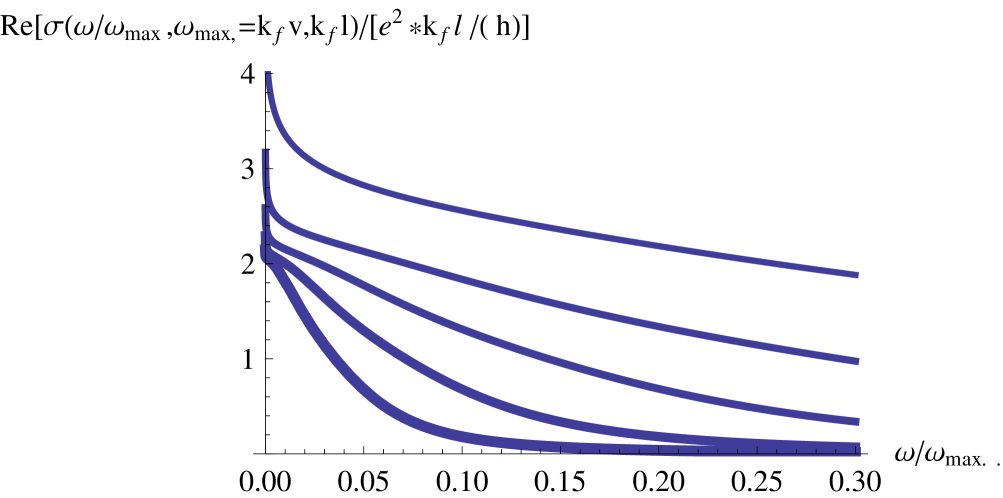
Figure 1: The conductivity as a function of the frequency for three cases: $k_{F}l=20$ (the lower graph), $k_{F}l=10$ $k_{F}l=5$ ,$k_{F}l=2.5$, $k_{F}l=1$ (the upper graph).

IV. Possible Experimental verification of the theory

One of the difficulties in measuring the surface conductivity is the fact that the bulk electrons contribute to the conductivity. The bulk electrons form a three dimensional $TI$ characterized by the inverted gap $\Delta$. For the case that the chemical potential $\mu>\Delta$ the ”‘ bulk”’ $TI$ will form a conduction band. For this case the spinor will be given by $\Psi(\vec{r})=\sqrt{v}\sum_{\sigma=\uparrow,\downarrow}\sum_{\vec{k}}e^{i\vec{k}\cdot\vec{r}}C_{\sigma}(\vec{k})U_{\sigma}^{(+)}(\vec{k})$. In contrast to the surface case the particles carry two spin polarizations. As a result the Hamiltonian for this case will be replaced by:

$$H^{(3D)}=\sum_{\sigma=\uparrow,\downarrow}\sum_{\vec{k}}(\hbar v(\sqrt{k^{2}+\Delta^{2}})-\mu)\hat{C}_{\sigma}^{\dagger}(\vec{k})\hat{C}_{\sigma}(\vec{k})+\sum_{\vec{k}}\sum_{\vec{p}}\sum_{\sigma=\uparrow,\downarrow}\sum_{\sigma^{\prime}=\uparrow,\downarrow}v\hat{C}_{\sigma}^{\dagger}(\vec{k})\Gamma_{\sigma,\sigma^{\prime}}(\vec{k},\vec{p})\hat{C}_{\sigma^{\prime}}(\vec{p}),$$ (49)

where $\Gamma_{\sigma,\sigma^{\prime}}(\vec{k},\vec{p})$ is the scattering matrix.Using a model of parallel resistors we find that the conductivity will be dominated by the bulk contributions. In order to observe the surface conductivity we need to be in a situation where $\mu<\Delta$. For this case the bulk will be insulating and the conductivity will be dominated by the surface part. For this case electronic Raman scattering might be a good tool to observe the surface conductivity. This might work for laser frequencies $\omega_{L}$ which excite the surface but not the bulk $\Delta>\omega_{L}>\mu$. In order to evaluate the Raman intensity we integrate out the anti-particles and obtain the effective two photon Hamiltonian:

$$H^{(ext.2)}=\int\frac{d^{2}k}{(2\pi)^{2}}\int\frac{d^{2}q}{(2\pi)^{2}}\int\frac{d^{2}q^{\prime}}{(2\pi)^{2}}\int\frac{d\omega}{2\pi}\Big{[}\frac{(ev)^{2}W^{(p,a)}_{i}(\vec{k}+\vec{q},-\vec{k})W^{(a,p)}_{j}(-\vec{k},\vec{k}-\vec{q}^{\prime})}{(\omega-\mu-(E(\vec{k}+\mu))}\Big{]}$$

$$C^{\dagger}(\vec{k}+\vec{q},\omega+\omega_{L}+\omega_{S})C(\vec{k}-\vec{q}^{\prime},\omega)A_{i}(-\vec{q},-\omega_{L})A_{j}(-\vec{q}^{\prime},-\omega_{s}),$$

where $A_{i}(-\vec{q},-\omega_{L})$ is the laser vector potential in the $i$ direction, $A_{j}(-\vec{q}^{\prime},-\omega_{s})$ is the scattering laser frequency and $W^{(p,a)}_{i}(\vec{k}+\vec{q},-\vec{k})$ represent the photon vertex which couples to electrons and holes. Taking the limit $\vec{q}\rightarrow 0$ we observe that the Raman frequency $\Omega=\omega_{L}-\omega_{S}$ can provide information about the electronic conductivity. The Raman spectrum measured in Conder is given by: $S(\Omega)=\frac{1}{\pi}[1+(e^{\beta\Omega}-1)^{-1}]Im.D[\Omega]$ where $D[\Omega]=\frac{-i}{L^{2}}\int_{0}^{\infty}\,dte^{i(\Omega+i\epsilon)t}\langle[\rho(t),\rho(0)]\rangle$ represents the chiral surface electronic density-density correlation. Since $Im.D[\Omega]$ is proportional to the conductivity $\sigma(\Omega)$, $Im.D[\Omega]\propto\Omega\sigma(\Omega)$, the Raman spectrum contains the information about the conductivity. For light the momentum $q$ is negligible and we can replace $W_{i}^{(p,a)}(\vec{k}+\vec{q},-\vec{k})\approx U_{i}(\vec{k})$, $W_{i}^{(a,p)}(-\vec{k},\vec{k}+\vec{q})\approx U^{*}_{i}(\vec{k})$ which represents the electronic spinor projection in the $i$ direction. Measuring the scattering light in the $j$ direction for an incoming light in the $i$ direction will be proportional to the density-density correlation ($i$ and $j$ correspond to the Cartesian coordinates on the surface of the $TI$, the incoming light vector $\vec{k}$ is almost perpendicular to the surface):

$$D_{j,i}[\vec{q},\Omega]=\int_{0}^{\infty}\,dte^{i\omega t}\int\frac{d^{2}k}{(2\pi)^{2}}\int\,\frac{d^{2}p}{(2\pi)^{2}}U_{j}(\vec{k})U_{i}(\vec{k})U^{*}_{j}(\vec{p})U^{*}_{i}(\vec{p})\langle C^{\dagger}(\vec{k}+\vec{q},t)C(\vec{k},t)C^{\dagger}(\vec{p}+\vec{q},t)C(\vec{p},0)\rangle].$$ (51)

The chiral properties of the surface electrons are probed with polarized light Conder . The circular polarized light $e^{\eta}$, $\eta=\pm$ is expressed in terms of the linear polarization $\epsilon^{1}(\vec{k})$, $\epsilon^{2}(\vec{k})$. The chiral correlation function $D_{-,+}[\vec{q},\Omega]$ is given in terms of the linear polarized light and spinors $U_{i}(\vec{k})$:

$$D_{-,+}[\vec{q},\Omega]=(D_{x,x}[\vec{q},\Omega]-D_{y,y}[\vec{q},\Omega])+i(D_{x,y}[\vec{q},\Omega]-D_{y,x}[\vec{q},\Omega]),$$

$$U_{i}(\vec{k})=\delta_{i,x}\sin[\chi(k_{x},k_{y}]-\delta_{i,y}\cos[\chi(k_{x},k_{y}]$$

$$Im.\sum_{i=x,y}\sum_{j=x,y}D_{j,i}[\vec{q}\rightarrow 0,\Omega]\propto\Omega\sigma(\Omega).$$

In Fig. 2 we plot the function $D[\vec{q}\rightarrow 0,\Omega]\propto\Omega\sigma(\Omega)$ using the conductivity given in Fig. 2. $k_{F}l=15$ (the lower graph), $k_{F}l=10$, $k_{F}l=5$(upper graph). The line shape in Fig. 2 is in qualitative agreement with the Raman line shift reported in ref Conder .

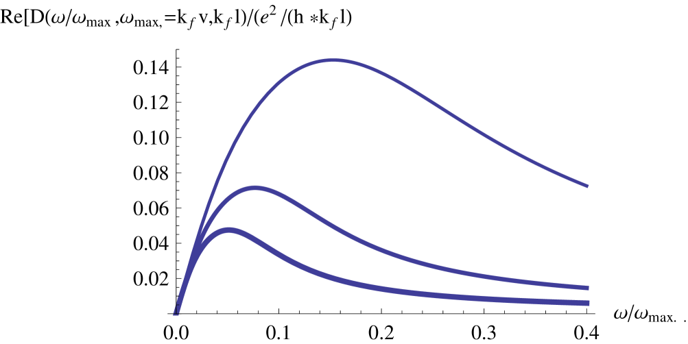
Figure 2: The Raman shift $D[\vec{q}\rightarrow 0,\Omega]\propto\Omega\sigma(\Omega)$ for $k_{F}l=5$, $k_{F}l=10$ , $k_{F}l=15$

VIII Conclusions

To conclude we have computed the conductivity for the conduction electrons on the surface of the $TI$ in the presence of a large chemical potential. Due to the $TI$ topology the conduction band contains a half vortex at $\vec{k}=0$. As a result the return probabilty vanishes and the quantum corrections are given by anti-localization effect as predicted for the symplectic ensemble. Using this theory we discuss the implications to the Raman scattering recently observed in $Bi_{2}Se_{3}$.

References

(1) B.A, Volkov and O.A. Pankratov, JETP Lett. 61, 2015 (1988).
(2) C.L. Kane and E.J. Mele, Phys. Rev. Lett.75, 146802 (2005).
(3) Xiao-Liang Qi and Shou-Cheng-Zhang, Rev. Modern Physics 83, 1057 (2011).
(4) D. Schmeltzer Phys.Rev.B 73, 165301 (2006); Advances in Condensed Matter and Material Research, Editors Hans Geelvinck and Sjaak Reyst , volume 10, chapter , pages (2011).
(5) D. Culcer cond-mat/1108.3076.
(6) R. Biswas and A.V. Balatsky,. Phys. Rev. B 81, 23405 (2010).
(7) Shinobu Hikami, Phys. Rev. B24, 2671 (1981).
(8) Hidekatsu Suzura and Tsuneya Ando, Phys.Rev.Let. 108,076804 (2002) and (preprint 2011).
(9) G. Thackhov and E.M. Hankiewicz, cond-mat v4.
(10) Zohar Ringel, Yaacov E. Kraus, and Ady Stern, Phys. Rev. B.86, 045102 (2012).
(11) Hai-Zhou Lu, Junren Shi, and Shun-Qing Shen, cond-mat v3.
(12) Ion Garate and Leonid Glazman, Phys. Rev. B 86, 035422 (2012).
(13) S. Raghu, S.B. Chung, X.L. Qi, and S.-C. Zhang, Phys. Rev. Lett. 104,116401 (2010).
(14) Michelle Maggiore, A modern Introduction to Quantum Field Theory, (Oxford Univrsity Press, 2005).
(15) A.A. Abrikosov, L.P. Gorkov, and I.E. Dzyaloshinski, Methods of Quantum Field Theory In Statistical Physics, ‘page 63. (Dover publications, 19–).
(16) J. Rammer, Quantum Field Theory of Non-Equilibrium States, pages 377-389, (Cambridge University Press 2007).
(17) G.Bergmann Phys.Rev.B 28,2914 (1983)
(18) D.Schmeltzer and M.Kaveh J.Phys.C 20,L175 (1987);Phys.Rev.B 37,9057 (1987)
(19) V. Gnezdilov, Yu. G. Pashkevich, H. Berger, E. Pomjakushina, K. Conder, and P.Lemmens, cond-mat .
(20) S. Donaich and E.H. Sondheimer, Green’s Functions for Solid State Physicists, (Imperial College Press, 1988).