Testing different methods for atmospheric parameters determination. The case study of the Am star HD 71297

Abstract

In this paper we present a detailed spectroscopic analysis of the suspected marginal Am star HD 71297. Our goal is to test the accuracy of two different approaches to determine the atmospheric parameters effective temperature, gravity, projected rotational velocity, and chemical abundances. The methods used in this paper are: classical spectral synthesis and the Versatile Wavelength Analysis (VWA) software.

Since our star is bright and very close to the Sun, we were able to determine its effective temperature and gravity directly through photometric, interferometric, and parallax measurements. The values found were taken as reference to which we compare the values ​​derived by spectroscopic methods. Our analysis leads us to conclude that the spectroscopic methods considered in this study to derive fundamental parameters give consistent results, if we consider all the sources of experimental errors, that have been discussed in the text. In addition, our study shows that the spectroscopic results are quite as accurate as those derived from direct measurements.

As for the specific object analyzed here, according to our analysis, HD 71297 has chemical abundances not compatible with the previous spectral classification. We found moderate underabundances of carbon, sodium, magnesium, and iron-peak elements, while oxygen, aluminum, silicon, sulfur, and heavy elements (Z $\geq$ 39) are solar in content. This chemical pattern has been confirmed by the calculations performed with both methods.

1 Introduction

The current era is characterized by an enormous growth of stellar data of different nature. The advent of space missions, such as CoRoT (Convection, Rotation and planetary Transits; Baglin et al., 2007) and Kepler (Borucki et al., 1997), designed to obtain precise photometry for an impressive number of stars, have led astronomers to undertake several ground-based spectroscopic campaigns in order to get as accurate as possible fundamental parameters such as effective temperature, surface gravity, projected rotational velocity, and metallicity. The analysis of this huge amount of data is possible, on reasonably short timescales, only through the use of automatic or semi-automatic procedures.

Among the various targets observed by Kepler, Am stars are assuming an ever growing importance. In fact, it was once thought that Am stars did not pulsate, and that the explanation for this is that atomic diffusion is expected to drain helium from the Heii driving zone. More intensive observations have revealed that this picture is not correct and several Am stars are known to pulsate from ground-based observations (based on superWASP photometry, see Smalley et al., 2011) as well as from Kepler satellite data (see Balona et al., 2011). In this last paper, the authors showed that an accurate measure of the location of the pulsating Am stars in the HR diagram is crucial to pin down effectively the pulsation models and to put observational constraint on the instability strip for pulsation in Am stars. However, for most of the investigated objects, a modern determination of the stellar parameters such as effective temperatures, gravities and chemical abundances, based on high resolution spectroscopy is still lacking. To fill this gap, we have already started a spectroscopic campaign devoted to obtain high resolution spectra of Am stars, being the first data obtained with the spectrograph SARG installed at the Italian telescope TNG. Our purpose in the near future is to analyze this growing amount of spectra to derive accurate stellar parameters for the investigated objects in the shortest possible time.

There are several examples in the literature of papers regarding various methods for automatic (or semi-automatic) spectroscopic analysis, (Tkachenko et al., 2012; Lehmann et al., 2011; Niemczura et al., 2009; Erspamer & North, 2003). However, it is important to ascertain the accuracy of the derived parameters obtained using different methods. A few recent papers have partially addressed this problem, reporting that significant differences can be found both in the derived stellar parameters (see e.g. Fossati et al., 2011) and/or in the estimated uncertainties in these quantities (see e.g. Molenda-Żakowicz et al., 2010).

With the aim of understanding how accurately we can derive the stellar parameters and the HR location for our sample of Am stars, we decided to concentrate our efforts on comparing the results that can be obtained by analyzing the high resolution spectrum for one star in our sample with the two methods available to us: i) classical spectral synthesis (see Catanzaro et al., 2011; Catanzaro & Balona, 2012, and references therein) and ii) Versatile Wavelength Analysis (VWA) (see Bruntt et al., 2010a, b, and references therein).

To carry out this exercise, we choose to analyze in detail the Am star HD 71297. This is the most suitable object in our sample because it is very bright (V = 5.58 mag) and the SARG@TNG spectrum has a very good signal-to-noise ratio. Moreover, HD 71297’s brightness allowed us to find very useful observational data in the literature, including an accurate Hipparcos parallax and interferometric measures which allow us to estimate independently from spectroscopy the stellar parameters. Thus, the main goal of this paper is to ascertain if the two quoted methods of quantitative spectral analysis lead to different or, on the contrary, to comparable results when used to exploit exactly the same observational material.

2 The target. The Am: star HD 71297

HD 71297 has been classified as suspected marginal Am star by Cowley (1968), with a spectral type of A5m: (colon denoted its marginal nature). We remind readers the definition of marginal Am star as an Am star in which there is a difference of less than five subclasses between the K-line and the metal line spectral types, and in which the line strength anomalies are mild. Cowley (1968) concluded that the star exhibits only weak metallic lines, looking like the spectrum of $\beta$ Ari. This classification has been confirmed one year later by Cowley et al. (1969).

Abt & Levy (1985) searched for binarity among a sample of 60 Am stars and concluded that HD 71297 may be variable in radial velocity with a period of a hundred days. They assigned the spectral type of kA8hA9mF0 to HD 71297.

This star has also been studied by Guthrie (1987) who derived atmospheric parameters, T_eff =7900 K, $\log g$=4.2, and calcium abundance, $\log N({\rm Ca})$ = 6.33, expressed in a scale in which $\log N(H)$ = 12.0, that is practically the solar value. Later on, Kuenzli & North (1998) revisited the star, finding it a little bit cooler and less evolved, T_eff =7712 K and $\log g$=4.06, but still with solar calcium abundance.

No other studies have been found in the recent literature, especially no detailed analysis of the chemical pattern of its atmosphere. Thus, we chose this object as a benchmark for the two methods of analysis we would like to compare in this paper.

Table 1: Evaluations of T_eff and $\log g$ values of HD 71297 on the basis of various photometric systems (see text for details).

Photometry	Teff	$\log g$	Calibration
$uvby$–$\beta$	7700$\pm$40	4.06$\pm$0.04	Napiwotzki et al. (1993)
$uvby$–$\beta$	7970$\pm$30	4.28$\pm$0.04	Ribas et al. (1997)
$UBVB_{1}B_{2}V_{1}G$	7770$\pm$80	4.46$\pm$0.06	Kuenzli & North (1998)
$uvby$–$\beta$	7770$\pm$125	4.08$\pm$0.125	Smalley & Kupka (1997)
$uvby$–$\beta$	7800$\pm$125	4.06$\pm$0.125	Heiter et al. (2002) MLT $\alpha$=0.5
$uvby$–$\beta$	7780$\pm$125	4.06$\pm$0.125	Heiter et al. (2002) using Canuto, Goldman & Mazzitelli (1996)

3 Observation and data reduction

Spectroscopic observations of HD 71297 were carried out with the SARG spectrograph, which is installed at the Telescopio Nazionale Galileo, located in La Palma (Canarias Islands, Spain). SARG is a high-resolution cross-dispersed echelle spectrograph (Gratton et al., 2001) that operates in both single-object and longslit (up to 26) observing modes and covers a spectral wavelength range from 370 nm up to about 1000 nm, with a resolution ranging from R = 29 000 to 164 000.

Our spectra were obtained on 2011, February 21 at R = 57 000 using two grisms (blue and yellow) and two filters (blue and yellow). These were used in order to obtain a continuous spectrum from 3600 Å to 7900 Å with significant overlap in the wavelength range between 4620 Å and 5140 Å. We acquired the spectra for the star with an exposure time of 120 sec. and a signal-to-noise ratio S/N of at least 100 per pixel in the continuum. For example, in the region centered around the Mgi triplet at 5170 Å the measured S/N is about 120.

The reduction of all spectra, which included the subtraction of the bias frame, trimming, correcting for the flat-field and the scattered light, the extraction for the orders, and the wavelength calibration, was done using the NOAO/IRAF packages. The IRAF package rvcorrect was used to make the velocity corrections due to Earth’s motion to transform the spectra to the barycentric rest frame.

4 Stellar parameters from photometry, interferometry and parallax.

Before starting with the analysis of the spectrum of HD 71297, it is extremely important to estimate the stellar parameters, mainly T_eff and $\log g$, through independent methods, such as those based on intermediate-band photometry, parallax, interferometry etc. This is useful to have: i) a reliable starting point for the spectroscopic analysis and ii) a trustworthy and accurate independent evaluation of the stellar fundamental parameters to compare with.

4.1 Evaluation of T_eff and $\log g$ from Strömgren and Geneva photometry

A first estimate of T_eff and $\log g$ for HD 71297 can be obtained from the Strömgren photometry: $V=5.607\pm 0.002$, $b-y=0.123\pm 0.002$, $m_{1}=0.197\pm 0.004$, $c_{1}=0.833\pm 0.006$, $\beta=2.831\pm 0.003$ (Hauck & Mermillod, 1998). However, It is important to check the value of $V$-band magnitude because HD 71297 is a (low-amplitude) variable star (see Balona et al., 2011). A safe average $V$ magnitude can be derived from the time-series photometry in the Hipparcos ($H_{p}$) and Tycho ($V_{T}$) photometric systems. Including the uncertainties in the trasformations to the Johnson $V$ system (Bessell, 2000), we get $V$=5.59$\pm$0.01 mag and $V$=5.60$\pm$0.01 mag. Finally, an additional independent measure was reported by Kuenzli & North (1998) who measured $V$=5.604$\pm$0.008 mag. On this basis, we adopted a value of $V$=5.60$\pm$0.01 mag for HD 71297. This value is consistent within the errors with all the above quoted evaluations.

The other Strömgren indices should be less uncertain with respect to $V$-band, however it is likely that the errors are somewhat underestimated.

We adopted an updated version of the TempLogG software (Rogers, 1995) to estimate T_eff and $\log g$ by using the calibrations present in the package. We did not consider the older calibration by Balona (1984) and Moon (1985); Moon & Dworetsky (1985), but only the more recent ones by Napiwotzki et al. (1993); Ribas et al. (1997); Kuenzli & North (1998). Note that the last calibration is for the Geneva $UBVB_{1}B_{2}V_{1}G$ system, whose photometry for HD 71297 is provided by Rufener (1988). These results are summarized in the first three rows of Table 1. In addition, we considered the results by Smalley & Kupka (1997) and Heiter et al. (2002) who provided $uvby$ grids based on the Kurucz model atmospheres but with different treatment of the convection. In particular we report on Table 1 the T_eff and $\log g$ estimated by interpolating the Smalley & Kupka (1997) grids that were built using the Canuto & Mazzitelli (1991) convection treatment. Similarly, the last two column of Table 1 list the stellar parameters obtained using two choices for the grids by Heiter et al. (2002): i) standard mixing-lenght theory (MLT) with $\alpha$=0.5; ii) the Canuto, Goldman & Mazzitelli (1996) treatment of the convection. In all these cases the error associated to the parameters was imposed as half-the width of the grid. An inspection of Table 1 reveals some dispersion among the various calibrations both in T_eff and $\log g$, even if the last three values are absolutely equivalent within the errors. Quantitatively, a simple average of the results gives: $\langle$T_eff$\rangle$=7800$\pm$90 K and $\langle$$\log g$$\rangle$=4.17$\pm$0.17 dex.

As for the interstellar reddening, TempLogG gives as a result $E(b-y)$=0.009$\pm$0.003 mag. This value is probably non-significant, because of the very low value of both reddening and associated uncertainty (underestimated in our opinion). Since the star is only 50 pc far from the Sun (see next sub-section), it is acceptable to neglect the effect of the interstellar absorption. This assumption was also confirmed a posteriori by looking into the spectrum of HD 71297 for the interstellar Nai lines at 5890.0, 5895.9 Å which can be used to estimate the interstellar reddening (see Munari & Zwitter, 1997). Indeed, these lines are practically undetectable. To conclude, in the following analysis we have neglected the interstellar reddening.

4.2 Evaluation of the stellar parameters from Photometry, Parallax and Interferometry

The Hipparcos parallax for HD 71297, $\pi$ = 19.99 $\pm$ 0.38 mas (van Leeuwen, 2007), allows us to estimate with the excellent accuracy of 2% the distance of this object: d = 50 $\pm$ 1.0 pc. It is then straightforward to calculate the visual absolute magnitude of the target: $M_{V}=2.105\pm 0.045$ mag. To derive the luminosity we need to evaluate first the visual bolometric correction BC_V. To this aim we adopted the models by Bessell, Castelli & Plez (1998) where it is assumed that M_bol,⊙ = 4.74 mag. We then get BC_V = 0.03 $\pm$ 0.01 mag for HD 71297. We note that to obtain this value we interpolated the Bessell, Castelli & Plez (1998) tables by using as input the T_eff and $\log g$ obtained from the photometry. The error was conservatively assumed to be 0.01 mag to take into account the observed dispersion of the photometrically derived T_eff and $\log g$. We have now estimated all the quantities needed to calculate the luminosity of HD 71297: $\log(L/L_{\odot})=1.04\pm 0.02$.

Table 2: Astrophysical quantities for HD 71297 evaluated independently from spectroscopy.

Parameter	Value
$\pi$	$19.99\pm 0.38$
$\alpha$	0.367$\pm$0.025
MV (mag)	$2.105\pm 0.045$
Mbol (mag)	$2.14\pm 0.04$
Teff (K)	$7810\pm 90$
$\log(L/L_{\odot})$ (dex)	$1.04\pm 0.02$
$\log g$ (dex)	$4.17\pm 0.06$
R/R⊙	$1.97\pm 0.14$
$M/M_{\odot}$	$1.77^{+0.12}_{-0.19}$
age (Myrs)	$790\pm 90$

Another very important piece of information is represented by the angular diameter of HD 71297, which was published by Lafrasse et al. (2010): $\alpha$ = 0.367 $\pm$ 0.025 mas. By using this value, together with the distance derived from Hipparcos parallaxes, d = 50 $\pm$ 1 pc, it is straightforward to evaluate the radius of our target: R = 1.97$\pm$0.14 R_⊙.

With the observational data available for HD 71297, the most convenient way to estimate the effective temperature is from the definition of surface brightness as given in Eq. 14.8 of Gray (2005). After simple algebra, we get:

$$\log T_{\rm eff}=c-0.1\cdot V+0.1\cdot BC-0.5\log\theta_{R}$$ (1)

where $\theta_{R}$ is the angular radius in arcsec and c is a constant given by:

$$c=\log T_{\rm eff}^{\odot}+0.1\cdot m_{V}^{\odot}-0.1\cdot BC_{\odot}+0.5\log\theta_{R}^{\odot}$$ (2)

To estimate $c$ we used the Sun “constants” reported by Bessell, Castelli & Plez (1998): $T_{\rm eff}^{\odot}$ = 5781$\pm$4 K, $m_{V}^{\odot}$ = $-$26.76$\pm$0.01 mag, $BC_{\odot}$ = $-$0.07$\pm$0.01 mag, and $\theta_{R}^{\odot}$ = 959.61$\pm$0.01 arcsec. Thus c = 2.58405$\pm$0.00140, and, from Eq. 1: $T_{\rm eff}$ = 7850 $\pm$ 280 K. In the error budget the most important contributor is the angular radius (diameter) at the $\sim$3.5% level, being the contribution of the other quantities practically negligible. The effective temperature value derived here is almost indistinguishable from that estimated directly from Strömgren and Geneva photometry, but with a larger uncertainty. Nevertheless, this evaluation appears robust, since it is based on different kind of independent measures (photometry, interferometry). Moreover, also the uncertainty can be calculated in a reliable and physical way. Hence, we decided to take a weighted average of the effective temperatures obtained with the two methods as the value to be used as a reference for comparison with spectroscopy. As a results, we obtain $T_{\rm eff}=7810\pm 90$K.

To estimate $\log g$, it is convenient to use the following expression that can be easily derived from the definition of $g$ and from the Stefan-Boltzmann relation:

$$logg = 4\log(T_{\rm eff}/T_{\rm eff}^{\odot})+\log(M/M^{\odot})+2\log(\pi)$$ (3)

$$+0.4(V+BC_{V}+0.26)+4.44$$

Where the various terms of the equation have the usual meaning and $M/M^{\odot}$ is the ratio mass of the star over mass of the Sun. Before using Eq. 3, we have to evaluate the mass of HD 71297. This can be safely done by adopting the calibration mass–$M_{V}$ (valid for luminosity class V stars) by Malkov (2003) that was derived on the basis of a large sample of eclipsing binaries stars. Hence, by using our $M_{V}$ estimate, we evaluated $\log(M/M^{\odot})=0.248\pm$ 0.05 dex (or $M/M^{\odot}=1.77^{+0.12}_{-0.19}$), where the error is largely conservative and completely dominated by the dispersion of the mass–$M_{V}$ relation.

Finally, applying Eq. 3 we obtain $\log g$ = 4.17 $\pm$0.06, again, in excellent agreement with the purely photometric evaluation but with a much smaller uncertainty. We will then use this value for comparison with spectroscopy.

Before closing this section, for completeness, it is worth estimating the age of HD 71297, taking advantage of the $\log T_{\rm eff}$ and $\log(L/L_{\odot})$ values estimated in this section. The location of the star in the HR diagram, together with some evolutionary tracks computed for the solar metallicity Z = 0.019 (Girardi et al., 2000), is shown in Fig. 1. Also shown are isochrones computed by Marigo et al. (2008) for the same Z (= 0.019) and for ages ranging from $\log t$ = 8.85 to 8.95, in steps of 0.05 ($t$ in years). The location of the star indicates a mass of M $\approx$1.75 $\pm$ 0.05 M_⊙ (in perfect agreement with the value adopted above) and an age of $t\approx$ 790 $\pm$ 90 Myrs.

In Table 2 we summarized all the astrophysical quantities for HD 71297 evaluated independently from spectroscopy.

Figure 1: Location of HD 71297 in the HR diagram together with evolutionary tracks and isochrones for $\log t$ ranging from 8.85 to 8.95 (step 0.05 and $t$ in yrs).

5 Atmospheric parameters from spectroscopy

In this section we will present separately the results from the analysis of the high resolution spectra of HD 71297 as obtained with the two different approaches quoted in the introduction. We want to stress that the two analysis have been performed by using the same spectrum, prepared as described in Section 3. In this way, we can be sure that any differences arising during the analysis will not be attributed to the quality of the data, but directly to the method itself.

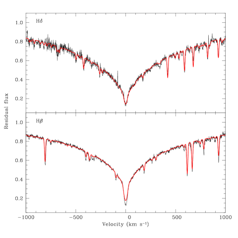
Figure 2: Observed H_β and H_δ with over-imposed the synthetic ones computed with the fundamental parameters derived in this section.

5.1 Stellar parameters and abundance analysis with classical spectral synthesis

This approach was already discussed in Catanzaro et al. (2011); Catanzaro & Balona (2012) and references therein. Thus, here we briefly summarize the principal features of this method. In order to determine the optimal parameters, we minimize the difference between the observed and synthetic spectrum. Thus we minimize

$$\chi^{2}=\frac{1}{N}\sum\left(\frac{I_{\rm obs}-I_{\rm th}}{\delta I_{\rm obs}}\right)^{2}$$

where $N$ is the total number of points, $I_{\rm obs}$ and $I_{\rm th}$ are the intensities of the observed and computed profiles, respectively, and $\delta I_{\rm obs}$ is the photon noise. Synthetic spectra were generated in three steps. First, we computed a LTE atmospheric model using the ATLAS9 code (Kurucz, 1993a). The stellar spectrum was then synthesized using SYNTHE (Kurucz & Avrett, 1981). Finally, the spectrum was convolved with the instrumental and rotational profiles.

As starting values of T_eff and $\log g$, we used the values derived in the previous section.

To decrease the number of parameters, we computed the $v\sin i$ of HD 71297 by matching synthetic line profiles from SYNTHE to a number of metallic lines. The Mgi triplet at $\lambda\lambda$5167-5183 Å was particularly useful for this purpose. The best fit was obtained for $v\sin i$ = 7.0 $\pm$ 0.5 km s^-1. This value is slightly lower than the one published by Royer et al. (2002) of $v\sin i$ = 11 km s^-1.

Uncertainties in T_eff, $\log g$, and $v\sin i$ were estimated by the change in parameter values which leads to an increases of $\chi^{2}$ by unity (Lampton et al., 1976).

To determine stellar parameters as consistently as possible with the actual structure of the atmosphere, we performed the abundance analysis by the following iterative procedure:

(i) $T_{\rm eff}$ is estimated by computing the ATLAS9 model atmosphere which gives the best match between the observed H_β and H_δ lines profile and those computed with SYNTHE (see Fig. 2). The model was computed using solar opacity distribution function (ODF) and microturbulence velocity $\xi$ = 2.4 $\pm$ 0.5 km s^-1, the latter value has been calculated following the calibration $\xi\,=\,\xi(T_{\rm eff},\log g)$ published by Allende Prieto et al. (2004). These two lines are the only useful for our purpose since they are located far from the echelle orders edges so that it was possible to safely recover the whole profiles. The simultaneous fitting of two lines led to a final solution as the intersection of the two $\chi^{2}$ iso-surfaces. Another source of uncertainties is due to the difficulties in normalization as is always challenging for Balmer lines in echelle spectra. We quantified the error introduced by the normalization in at least 100 K, that we summed in quadrature with the error obtained by the fitting procedure. The final result is:

$$T_{\rm eff}\,=\,7500\,\pm\,180\,K$$

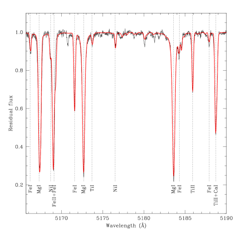
Figure 3: Observed Mgi triplet with over-imposed the synthetic one computed with the fundamental parameters derived in this section

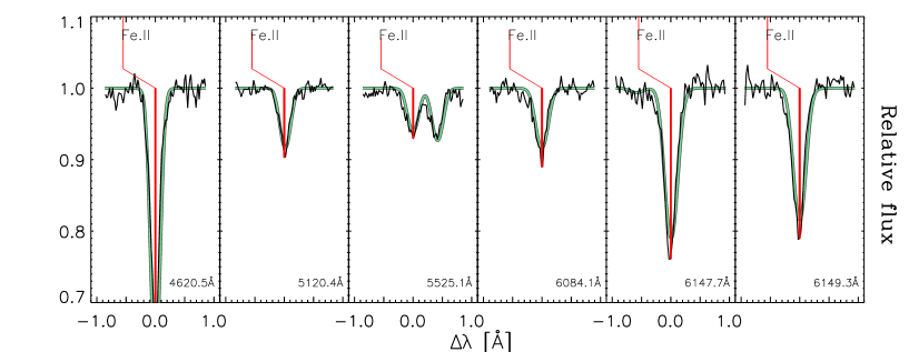
Figure 4: The figure shows six Feii lines in HD 71297 fitted by VWA (continuous line). The wavelengths of the fitted lines are given in the bottom right corner of each panel.

The surface gravity was estimated from line profile fitting of Mgi lines with developed wings. This method is based on the fact that the wings of the Mgi triplet at $\lambda\lambda$ 5167, 5172, and 5183 Å lines are very sensitive to $\log g$ variations. In practice, we have first derived the magnesium abundance through the narrow Mgi lines at $\lambda\lambda$ 4571, 5528, 5711 Å and the Mgii $\lambda$ 7877 Å, and then we fitted the wings of the triplet lines by fine tuning the $\log g$ value. The magnesium abundance we got from these lines was $\log Mg/N_{\rm tot}=-4.62\pm 0.14$.

To derive $\log g$ by fitting spectral wings is essential to take into account very accurate measurements of the atomic parameters of the transitions, i.e. $\log gf$ and the radiative, Stark and Van der Waals damping constants. Regarding $\log gf$ we used the values of Aldenius et al. (1997), Van der Waals damping constant is that calculated by Barklem, Piskunov & O’Mara (2000) ($\log\gamma_{\rm Waals}\,=\,-7.37$), the Stark damping constant is from Fossati et al. (2011) ($\log\gamma_{\rm Stark}\,=\,-5.44$), and the radiative damping constant is from NIST database ($\log\gamma_{\rm rad}\,=\,7.99$).

This procedure results in the final value of:

$$\log g\,=\,4.0\,\pm\,0.1.$$

(ii) As a second step we determine the stellar abundances by computing a synthetic spectrum that reproduced the observed one. Therefore, we divide our spectrum into several intervals, 25 Å wide each, and derived the abundances in each interval by performing a $\chi^{2}$ minimization of the difference between the observed and synthetic spectrum. The minimization algorithm has been written in IDL language, using the amoeba routine. We adopted lists of spectral lines and atomic parameters from Castelli & Hubrig (2004), who updated the parameters listed originally by Kurucz & Bell (1995).

For each element, we calculated the uncertainty in the abundance to be the standard deviation of the mean obtained from individual determinations in each interval of the analyzed spectrum. For elements whose lines occurred in one or two intervals only, the error in the abundance was evaluated by varying the effective temperature and gravity within their uncertainties given in Table 3, $[T_{\rm eff}\,\pm\,\delta T_{\rm eff}]$ and $[\log g\,\pm\,\delta\log g]$, and computing the abundance for $T_{\rm eff}$ and $\log g$ values in these ranges. We found a variation of $\approx$ 0.1 dex due to temperature variation. We did not find any significant abundance change by varying $\log g$. The uncertainty in the temperature is the main error source on our abundances.

The derived abundances, expressed in terms of solar values (Grevesse et al., 2010), are shown in Fig. 6 (red dots). For all the chemical elements for which we detected spectral lines in our spectrum, we found moderate under-abundances with respect to the solar analogues, with the exception of the elements with high Z ($\geq$ 40), for which we found normal abundances.

As an example of our spectral synthesis we show in Fig. 3, the comparison between the observed spectral range from 5160 Å to 5190 Å and the synthetic one. In the second column of Table 3, we listed the abundances for our star derived with the method described above.

5.2 Stellar parameters and abundance analysis with VWA

The software package VWA relies on the iterative fit of synthetic profile regions around reasonably isolated absorption lines. VWA has a graphical user interface (GUI), which allows the user to investigate the spectra in detail, pick lines manually, inspect the quality of fitted lines, etc.

VWA uses data from various sources. In particular, for the calculation of synthetic spectra it uses the $SYNTH$ code by Valenti & Piskunov (1996), which works with $ATLAS9$ models, and atomic parameters and line-broadening coefficients from the $VALD$ database (Kupka et al., 1999). We note that we used model atmospheres interpolated in the fine grid published by Heiter et al. (2002). These models rely on the original ATLAS9 code by Kurucz (1993a) but use a more advanced convection description (Kupka, 1996) based on the works by Canuto & Mazzitelli (1992).

A thorough description of how VWA works can be found in Bruntt et al. (2004); Bruntt, De Cat & Aerts (2008). Here we only recall the main steps of the analysis.

• Normalization: the first step consists in an accurate normalization of the spectrum. This can be achieved by adopting a synthetic spectrum (with approximately the same stellar parameters as the target) as a template to properly identify (in the GUI) suitable regions to anchor the continuum of the observed spectrum.

• Setup and line selection: atomic parameters and a preliminary model are setup on the basis of initial values for the stellar parameters. The line selection can be carried out either in automatic or manual way. We first searched for good lines (i.e. with low blending) in an automatic way, then we checked the result visually line by line on the GUI.

• Fit of the lines and check of the result: each line is fitted by iteratively changing the abundance to match the equivalent width (EW) of the observed and calculated spectrum. The fitted lines are inspected in the GUI, problems with the continuum level or asymmetries in the line are readily identified, and these lines are discarded. This is done automatically by calculating the $\chi^{2}$ of the fit in the core and the wings of the lines. This is followed by a manual inspection of the fitted lines. Figure 4 displays a few selected lines and the relative fits to demonstrate the quality of the observed data (narrow lines) and the fit with VWA (thick lines).

• Iterative estimate of T_eff, $\log g$, and $\xi$: The atmospheric parameters and the microturbulence were then refined in several steps. This was done by minimizing the correlations between the abundance of [Fei/H] lines and equivalent width and excitation potential (EP), and requiring good agreement between the abundances of [Fei/H] and [Feii/H] (the difference in abundance: A(Fei) -A(Feii) is often referred as “ionization balance”). This task is accomplished by inspecting the results on the GUI and calculating the needed models as required (see Fig. 5).

• Chemical abundance: on the basis of the atmospheric parameters determined from [Fei/H] and [Feii/H], the mean abundances for all the elements with good lines can be finally calculated.

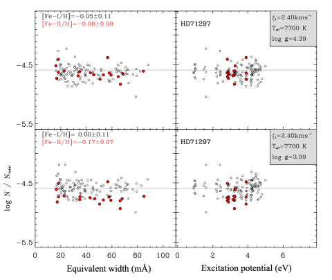
Figure 5: Abundance of Fe in HD 71297 for two different atmosphere models as a function of equivalent width (left panels) and excitation potential (right panels). Fei and Feii lines are plotted with open and solid points, respectively. The horizontal line in each panel show the value of log N_Fe/N_total=-4.53 adopted for the Sun, according to Grevesse et al. (2010). Top panels show the results for the adopted (best) parameters, while bottom panels display the effect of decreasing $\log g$ by 0.4 dex (see labels).

In Fig. 5 we show the abundances of Fe for the best model (T_eff=7700 $\pm$ 150 K; $\log g$=4.39 $\pm$ 0.06 dex; $v\sin i$= 7.0 $\pm$ 1 km s^-1 and $\xi$=2.4 $\pm$ 0.2 km s^-1) and for a model with $\log g$ decreased by 0.4 dex, i.e. a value approximately equal to that evaluated above with the Mgi triplet. The abundances are shown versus EW and EP. Open circles are Fei and solid circles are Feii lines, respectively. The mean abundance and rms scatter of Fei and Feii lines are given in each panel. We note that in the calculation of the ionization balance we adopt the rms of the mean, hence the uncertainties on the Fei and Feii abundances are significantly smaller (e.g. $\sim$ 0.01-0.02 dex). Bearing this in mind, a comparison of top and bottom panels in the figure clearly show that in the VWA framework a value $\log g\approx$ 4.0 dex is unlikely.

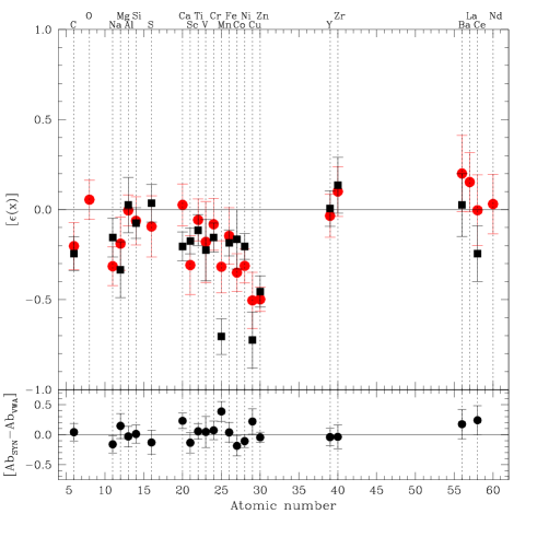
Figure 6: Chemical pattern for HD 71297 derived with the two different methods, red dots are from spectral synthesis and black squares from VWA. The bottom panel shows the difference between the two methods, for all the chemical elements in common.

To estimate the uncertainties of the atmospheric parameters, we repeated the above outlined analysis by varying significantly $T_{\rm eff}$, $\log g$ and $\xi$ (one parameter is allowed to vary while the other two are kept fixed). In this way we can determine when the correlations with EW and EP become significant or the ionization balance begins to deviate from equality (see Bruntt, De Cat & Aerts, 2008, for details). The same perturbed models can be used to estimate the uncertainty on the [Fe/H] value by estimating the variation on its value caused by 1 $\sigma$ perturbation of one parameter among T_eff, $\log g$, $\xi$ and taking fixed the other two (see Bruntt, De Cat & Aerts, 2008, for a detailed discussion). The resulting three uncertainties were summed in quadrature together with the rms scatter of Fei to obtain the final error on [Fe/H]. We underline that this method for the determination of the uncertainties gives only an internal estimate since the absolute temperature scale of the model atmospheres may be systematically wrong. Thus, our measures could show a good precision, but the accuracy is most likely not as good (Bruntt et al., 2010b).

It is important to note that one of the physical assumptions in the models adopted here is local thermodynamical equilibrium (LTE), but deviations from LTE start to become important for stars hotter than about 6300 K, especially for stars more metal poor than the Sun. Thus we have included the NTLE corrections in the present analysis according to Rentzsch-Holm (1996). The correction for neutral iron in our case is [Fei/H]${}_{\rm NLTE}=$ [Fei/H]${}_{\rm LTE}+0.11$ dex. When this correction is applied, Feii (unaffected by NLTE) must be increased by adding $+0.2$ to $\log g$. This correction has been applied in the results from VWA reported here.

The stellar parameters and the abundances for iron and the other measured chemical species obtained by means of VWA are shown in Table 3. The uncertainties were calculated as for iron but only for elements with at least three lines measured. For those chemical species for which less than three lines have been identified, we arbitrarily set the errors in 0.15 dex for elements with only one line and 0.10 dex for elements with two lines.

Table 3: Comparison among atmospheric parameters and abundances derived by spectral synthesis modeling and by VWA approach. $N$ denotes the number of lines used with VWA package. T_eff is in Kelvin, $\log g$ is in dex, while $v\sin i$ and $\xi$ are in Km/s. Abundances are expressed in the form $\log N_{\rm el}/N_{\rm Tot}$. An asterisk indicate that these uncertainties were re-determined in Sect. 6.

	Synthesis	VWA	N	Sun
Teff	7500 $\pm$ 180	7700 $\pm$ 150
$\log g$	4.0 $\pm$ 0.28∗	4.39 $\pm$ 0.20∗
$v\sin i$	7.0 $\pm$ 0.5	7.0 $\pm$ 1.0
$\xi$	2.4 $\pm$ 0.5	2.4 $\pm$ 0.2
C	$-$3.81 $\pm$ 0.12	$-$3.85 $\pm$ 0.08	7	$-$3.60 $\pm$ 0.05
O	$-$3.29 $\pm$ 0.10	—	-	$-$3.34 $\pm$ 0.05
Na	$-$6.11 $\pm$ 0.10	$-$5.95 $\pm$ 0.10	2	$-$5.79 $\pm$ 0.04
Mg	$-$4.62 $\pm$ 0.14	$-$4.77 $\pm$ 0.15	1	$-$4.43 $\pm$ 0.04
Al	$-$5.59 $\pm$ 0.08	$-$5.56 $\pm$ 0.15	1	$-$5.58 $\pm$ 0.03
Si	$-$4.59 $\pm$ 0.13	$-$4.60 $\pm$ 0.08	8	$-$4.52 $\pm$ 0.03
S	$-$5.00 $\pm$ 0.17	$-$4.88 $\pm$ 0.10	2	$-$4.91 $\pm$ 0.03
Ca	$-$5.62 $\pm$ 0.15	$-$5.90 $\pm$ 0.07	9	$-$5.69 $\pm$ 0.04
Sc	$-$9.19 $\pm$ 0.16	$-$9.06 $\pm$ 0.06	4	$-$8.88 $\pm$ 0.04
Ti	$-$7.14 $\pm$ 0.10	$-$7.20 $\pm$ 0.07	24	$-$7.08 $\pm$ 0.05
V	$-$8.28 $\pm$ 0.21	$-$8.33 $\pm$ 0.15	1	$-$8.10 $\pm$ 0.08
Cr	$-$6.48 $\pm$ 0.14	$-$6.55 $\pm$ 0.07	26	$-$6.39 $\pm$ 0.04
Mn	$-$6.92 $\pm$ 0.14	$-$7.31 $\pm$ 0.09	7	$-$6.60 $\pm$ 0.04
Fe	$-$4.68 $\pm$ 0.15	$-$4.72 $\pm$ 0.06	125	$-$4.53 $\pm$ 0.04
Co	$-$7.39 $\pm$ 0.08	$-$7.21 $\pm$ 0.15	1	$-$7.04 $\pm$ 0.07
Ni	$-$6.13 $\pm$ 0.08	$-$6.02 $\pm$ 0.06	26	$-$5.81 $\pm$ 0.04
Cu	$-$8.35 $\pm$ 0.15	$-$8.57 $\pm$ 0.15	1	$-$7.84 $\pm$ 0.04
Zn	$-$7.97 $\pm$ 0.04	$-$7.93 $\pm$ 0.07	2	$-$7.47 $\pm$ 0.05
Y	$-$9.86 $\pm$ 0.11	$-$9.82 $\pm$ 0.09	4	$-$9.82 $\pm$ 0.05
Zr	$-$9.35 $\pm$ 0.13	$-$9.32 $\pm$ 0.15	1	$-$9.45 $\pm$ 0.04
Ba	$-$9.65 $\pm$ 0.19	$-$9.83 $\pm$ 0.15	1	$-$9.85 $\pm$ 0.09
La	$-$10.78 $\pm$ 0.16	—	-	$-$10.93 $\pm$ 0.04
Ce	$-$10.46 $\pm$ 0.19	$-$10.70 $\pm$ 0.15	1	$-$10.45 $\pm$ 0.04
Nd	$-$10.58 $\pm$ 0.16	—	-	$-$10.61 $\pm$ 0.04

6 Comparison of the methods

In the previous section we have analyzed the high resolution spectrum of the Am: star HD 71297 using two different approaches: the classical spectral synthesis and VWA. The results for effective temperature, gravity, $v\sin i$, microturbulence, and chemical abundances, obtained with the two methods have been summarized in Tab. 3. We can now compare between them the stellar parameters obtained with the two quoted methods, taking also into account the completely independent results obtained in Sect. 4 for T_eff and $\log g$ as summarized in Tab. 2.

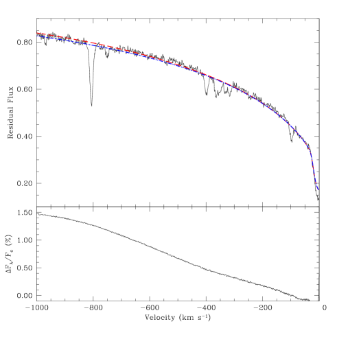
Figure 7: Upper panel - Comparison between observed and synthetic H$\beta$ profiles computed with two convection models represented by red dashed line (MLT) and by blue dot-dashed line (CM). Bottom panel shows the differences between normalized fluxes in H$\beta$ profile obtained from two models differing only by the convection treatment.

First of all, the atmospheric models we used in our calculations are both ATLAS9 based but with different convection zone treatments. In particular, in Sect. 5.1 it was computed using the classical treatment MLT with fixed $\alpha$=1.25 (Castelli et al., 1997). In Sect. 5.2, the model was interpolated in the fine grid by Heiter et al. (2002), which uses a more advanced convection description based on Canuto & Mazzitelli (1992) (CM).

Heiter et al. (2002) investigated the effects of the different convection approaches into the Balmer lines profiles and they concluded that the observed profiles should have an accuracy of at least 0.5 $\%$ to clearly appreciate the differences between convection models with different efficiency.

In order to quantify these effects on our target, we computed two synthetic H$\beta$ profiles using the same T_eff = 7700 K and $\log g$ = 4.39 but with different convection models. We show this comparison in Fig. 7, where in the upper panel we compare the observed blue wing of the H$\beta$ with overimposed the profiles computed with MLT (red dashed curve) and with CM treatment (blue dot-dashed line). In the bottom panel we report the difference in percentage between the two models. Since the maximum difference is of the order of 1.5 $\%$, indistinguishable at our level of signal-to-noise ratio, we conclude that for our target we can neglect the differences arising from the convection models adopted.

To verify the accuracy of this conclusion we have repeated the calculation for effective temperature, gravity, and abundances as described in Sect. 5.1. Again, we estimated T_eff by simultaneous fitting of H$\gamma$ and H$\delta$ but using ATLAS9 models modified for the CM treatment convection. We obtained T_eff = 7600 $\pm$ 150 K, that is closer to the photometric/interferometric value, but also totally consistent with the value derived adopting the MLT treatment for convection. Using this temperature, we estimated gravity fitting the Mgi triplet and we obtain $\log g$ = 4.10 $\pm$ 0.10, again compatible with previous value.

For what concerns the abundances, the model built with these values of effective temperature and gravity has been used to repeat the spectral synthesis analysis, adopting the same intervals as in Sect. 5.1. In Fig. 8 we displayed the differences between the abundances reported in Tab. 3 computed with MLT based model and those computed with CM model. Also in this case the results are consistent, being the weighted average of all differences equal to $-$0.01 $\pm$ 0.09.

Starting with T_eff, the classical spectral synthesis method and VWA agree well within 1 $\sigma$. There is also a 1.3 $\sigma$ agreement with the T_eff value estimated from photometry and interferometry, albeit the VWA value is closer by 200 K to the reference value. On the contrary, concerning the value of $\log g$, there is a significant discrepancy between the classical spectral synthesis method and VWA results: $\log g$ =4.0 $\pm$ 0.1 dex from synthesis of the strong Mgi triplet and $\log g$ =4.39 $\pm$ 0.06 dex from ionization equilibrium of Fei/Feii (VWA). The situation is even more complex if we take as a reference the gravity evaluated independently from spectroscopy in Sect. 2: $\log g$=4.17$\pm$0.05 dex. This value lies halfway between the two spectroscopy-based methods, being incompatible by more than 1 and 2 $\sigma$ with respect to the results of classical spectral synthesis and VWA methods, respectively. Thus, if we trust in interferometry and parallax we have to conclude that even high resolution spectroscopy is unable, at least in the case HD 71297, of evaluating the $\log g$ value better than 0.2 dex, being also the internal errors on this value underestimated for both methods.

Figure 8: Comparison between abundances computed using models that differ for the treatment of the convection theory, MLT vs CM.

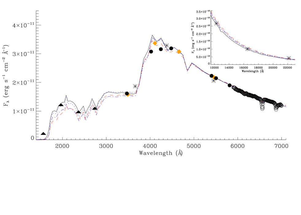
Figure 9: Comparison between observed spectral energy distribution and four theoretical fluxes. The meaning of the symbols is the following: triangles are TD1 fluxes, filled circles represent Geneva photometry, diamonds are fluxes from uvby magnitudes, asterisks are UBVJHK fluxes, and open circles represent the spectrophotometry. The theoretical distributions have been calculated for: T_eff= 7810 K and $\log g$= 4.17 (continuous black line), T_eff= 7700 K and $\log g$= 4.39 (CM model, dotted blue line), T_eff= 7500 K and $\log g$= 4.00 (MLT model, dashed red line), and T_eff= 7600 K and $\log g$= 4.10 (CM model, dash-dotted purple line)

To investigate further the accuracy of the results obtained with the two different spectroscopic analysis about T_eff and $\log g$, we built the Spectral Energy Distribution (SED) of HD 71297 (see Appendix for all the details on the construction of the SED) as shown in Fig. 9. The figure shows the comparison of the various photometric or spectrophotometric sources with three models (in different colors and line styles), as estimated in the previous sections. As well known, the Balmer jump is sensitive to surface gravity (as well as to effective temperature and line blanketing), hence looking at the UV part of the SED we can get some insight about the “best” couple (T_eff, $\log g$). Even a qualitative check on the figure show that the T_eff, $\log g$ couple evaluated in Sect. 4.1 (from parallax and interferometry) reproduces better the SED at all wavelength. In particular, in the far UV, the classical spectral synthesis method has the worse agreement due to the low T_eff, whereas across the Balmer Jump, VWA seems to have a too high $\log g$. This reflects the fact that both spectral synthesis and VWA methods go through a modeling that introduces errors, then it is important to discuss some of them.

The error we found in $\log g$ by fitting the wings of the Mgi triplet (i.e. 0.1 dex) is the formal error due to the fitting procedure. Actually there is at least another source of error that we have to discuss and consider. The result of the modeling of a spectral line depends essentially on the atomic parameters of the transition and in particular, for what concern the width of the spectral lines, we have to pay attention to the radiative, Stark and Van der Waals damping constants. The values of these three numbers set the broadening of the line and it is straightforward to understand the importance of their accuracy on the final value of $\log g$.

To focus our attention on this problem, we performed the following simulation: we fitted the observed profile of the Mgi $\lambda$5172.684 Å on synthetic profiles by varying the damping constants, one at a time, by an amount equal to their typical uncertainties. According to Barklem, Piskunov & O’Mara (2000), we adopted 5$\%$ as typical error in damping constants, obtaining that such a variation of $\gamma_{\rm Stark}$ and $\gamma_{\rm Waals}$ lead to an uncertainty in $\log g$ equal to $\approx\pm$ 0.3 dex. Similarly, a variation of $\gamma_{\rm rad}$ of 5%, lead to a $\approx\pm$ 0.15 dex uncertainty on $\log g$. Therefore, considering these errors as random and independent, we can conclude that the final uncertainties on gravity estimated by fitting the wings of one line is given from their quadratic sum and then equal to 0.45 dex. However, since we have applied this method to all the Mgi triplet, the final uncertainty coming from atomic parameters is 0.26 dex. Finally, considering also the formal error on the fitting procedure, we obtained the total error on $\log g$ equal to 0.28 dex. With such an error, $\log g$ derived with classical spectral synthesis is consistent with other values found in this study.

As for VWA, the estimate of $\log g$ by means of the ionization balance can be affected by over-ionization effects and uncertainties in the temperature structure of the model atmosphere, as well as to uncertainties on the atomic parameters (Fuhrmann et al., 1997). Thus, the formal error on $\log g$ we derived in our analysis has to be regarded as a lower limit for the true uncertainty on this parameter. Since it is difficult to estimate quantitatively the effect of the various source of uncertainty on the final value of $\log g$, we decided to assign a “typical error” of 0.2 dex. This suggestion is justified by the work of Bruntt et al. (2012) who used VWA to analyze high resolution spectra for 93 solar-type stars possessing accurate $\log g$ values measured by means of asteroseismological techniques on the basis of outstanding Kepler satellite photometry. These authors find an average difference $\log g({\rm spec})-\log g({\rm asteroseismic})$=+0.08$\pm$0.07 dex with a few objects showing larger discrepancies ($\sim$0.3 dex). Thus, an uncertainty of the order of 0.2 dex in $\log g$ is absolutely normal. A similar conclusion was reached by Smalley (2005): “Realistically, the typical errors on the atmospheric parameters of a star, will be T${}_{\rm eff}\pm$100 K (1$\sim$2%) for $\pm$0.2 dex ($\sim$20%) for $\log g$ ”. Finally, as for the values of $v\sin i$, $\xi$, and chemical abundances, an inspection of Tab. 3 reveals that there is a good agreement between spectral synthesis and VWA, in spite of the discrepancies in T_eff and $\log g$. The agreement in chemical abundance is not surprising. As argued by Smalley (2005), the atmospheric parameters obtained from spectroscopic methods alone may not be consistent with the “true” values as obtained by model-independent methods, but this is not necessarily important for abundance analyses of stars.

7 Conclusion

In this paper we have tested two different methods commonly used in the recent literature to characterize the stellar atmospheres and their chemical pattern: classical spectral synthesis and VWA package. This test was performed analyzing the spectrum of HD 71297 carried out with SARG@TNG. This object has been classified by Cowley (1968) as a suspected marginal metallic star, and later on Abt & Levy (1985) assigned the spectral type of kA8hA9mF0.

From direct measurements of distance and diameter, we obtained for our target the following astrophysical parameters: T_eff = 7810 $\pm$ 90 K and $\log g$ = 4.17 $\pm$ 0.05. As a by-product we were also able to derive estimation of R/R_⊙ = 1.97 $\pm$ 0.14, $M/M_{\odot}$ = 1.77${}^{+0.12}_{-0.19}$, and age = 790 $\pm$ 90 Myrs.

For what concern the main part of our paper, i.e. the comparison of the two different approaches, we can summarize as follows:

• Classical spectral synthesis method gives us the following values: T_eff = 7500 $\pm$ 180 K and $\log g$ = 4.10 $\pm$0.28 that are consistent with the previous values, at least within the errors. Projected rotational velocity has been evaluated in 7.0 $\pm$ 0.5 km s^-1 and $\xi$ = 2.4 $\pm$ 0.5 km s^-1. With these parameters, abundance analysis gives us a general underabundance of iron peak elements with the exception of calcium that is solar in content. Solar abundances are also shown by oxygen, yttrium, zirconium, barium and rare earths. We also tested the influence of the convection in the calculation of the synthetic spectrum. As in the case of VWA, we used Heiter et al. (2002) models to repeat the analysis, obtaining results totally consistent with those obtained with MLT theory as treated in Kurucz (1993a) with no overshooting and $\alpha$ = 1.25. Thus we conclude that, at least in the case of a star as hot as HD 71297, and for the resolution and SNR of our spectrum, the results are only slightly affected by the choice about the particular treatment of convection adopted for the analysis. The same conclusion is shared by Gardiner et al. (1999), who conclude that the MLT and CM models all give similarly reasonable results. On the contrary, for cooler targets the role of convection will be more significant and we will take it into account properly.

• By using VWA we obtained the following parameters: T_eff = 7700 $\pm$ 150 K and $\log g$ = 4.39 $\pm$0.06, a projected rotational velocity of 7.0 $\pm$ 1.0 km s^-1 and $\xi$ = 2.4 $\pm$ 0.2 km s^-1. Considering the experimental errors all these quantities are comparable with the ones derived with the others method. Also the abundances show a pattern similar to the one computed with classical spectral synthesis.

As a general conclusion we can state that the methods considered in this study to derive fundamental parameters useful to characterize stellar atmosphere give consistent results, if we consider all the sources of experimental errors.

An important result of this study concern the chemical pattern found for HD 71297. Contrary to what is expected from the previous classification, our abundances (reported in Tab. 3) do not look like those of normal Am star (see Fig. 5 in Catanzaro et al., 2011, for example). In fact, iron-peak elements show moderate underabundances, as well as carbon and sodium. Heavy elements like yttrium, zirconium, barium and rare earths, that usually in A-type stars display abundances greater than the Sun analogues (Erspamer & North, 2003), are quite normal in our target.

The results shown in this paper, concernin the consistency of classical spectral synthesis and VWA approaches to the analysis of stellar spectra, will allow us to confidently apply these codes to the other Am stars observed at SARG@TNG.

Appendix A Spectral Energy Distribution

The observed SED has been obtained by merging various data sources collected from the literature. In particular, the stellar flux shown in Fig. 9 was constructed by using the following data:

• UV fluxes taken from TD1 satellite (Thompson et al., 1978) that cover the 1565-2740 Å range;

• uvby magnitudes from Hauck & Mermillod (1998) and converted in physical units by using the calibrations given by Gray (1998); y magnitude has been derived from UBV color via the calibration of McSwain & Gies (2005)

• Geneva photometry taken from Rufener (1988) and converted in fluxes by means of the calibrations given by Rufener & Nicolet (1988);

• UBV magnitudes taken from Mermilliod (1991) and converted in fluxes using Bessell, Castelli & Plez (1998) calibrations;

• spectrophotometry in the range 5800-8000 Å taken from Weaver & Torres-Dodgen (1995);

• JHK magnitudes from 2MASS survey (Skrutskie et al., 2006), converted in physical units by using van der Bliek, Manfroid & Bouchet (1996).

As discussed in Sect. 4.1, we neglected the effects of interstellar reddening. In order to be consistent with the iron abundance we found in our previous analysis, each theoretical SED has to be calculated with an opacity ODF corresponding to a metalicity of [Fe/H] $=-0.15$. To achieve this goal, we computed for each couple of (T_eff, $\log g$) two synthetic fluxes, one for ODF=[0.0] and one for ODF=[-0.5] and then we interpolated between them.

References

- Abt & Levy (1985) Abt H. A., Levy S. G., 1985, ApJ, 59, 229
- Aldenius et al. (1997) Aldenius M., Tanner J. d., Johansson S., Lundberg H., Ryan S. G., 2007, A&A, 461, 767
- Allende Prieto et al. (2004) Allende Prieto C., Barkelm P. S., Lambert D. L., Cunha K., 2004, A&A, 420, 183
- Baglin et al. ( 2007) Baglin, A., Auvergne, M., Barge, P., et al. 2007, AIPC, 895, 201
- Balona (1984) Balona L. A., 1984, MNRAS, 211, 973
- Balona (1994) Balona L. A., 1994, MNRAS, 268, 119
- Balona et al. (2011) Balona L. A., Ripepi V., Catanzaro G., et al., 2011, MNRAS, 414, 792
- Barklem, Piskunov & O’Mara (2000) Barklem P. S., Piskunov N., O’Mara B. J., 2000, A&AS, 142, 467
- Bessell (2000) Bessell M. S. 2000, PASP, 112, 961
- Bessell, Castelli & Plez (1998) Bessell M. S., Castelli F., Plez B., 1998, A&A, 333, 231
- Borucki et al. (1997) Borucki W.J., Koch D.G., Dunham E.W., et al., 1997, ASP Conf. Ser. 119, 153
- Bruntt et al. (2004) Bruntt H., Bikmaev I. F., Catala C., et al. 2004, A&A, 425, 683
- Bruntt, De Cat & Aerts (2008) Bruntt H., De Cat P., & Aerts C. 2008, A&A, 478, 487
- Bruntt (2009) Bruntt H. 2009, A&A, 506, 235
- Bruntt et al. (2010a) Bruntt H., Deleuil M., Fridlund M., et al. 2010a, A&A, 519, 51
- Bruntt et al. (2010b) Bruntt H., Bedding T. R., Quirion P.-O., et al. 2010b, MNRAS, 405, 1907
- Bruntt et al. (2012) Bruntt H., Basu S., Smalley B., Chaplin W.J., Verner G.A., et al. 2012, 423, 122
- Canuto & Mazzitelli (1991) Canuto V. M. & Mazzitelli I. 1991, ApJ, 370, 295
- Canuto & Mazzitelli (1992) Canuto V. M. & Mazzitelli I. 1992, ApJ, 389, 724
- Canuto, Goldman & Mazzitelli (1996) Canuto V. M., Goldman I., Mazzitelli I. 1996, ApJ, 473, 550
- Castelli et al. (1997) Castelli F., Gratton R., Kurucs R. L., 1997, A&A, 318, 841 (erratum: 1997, A&A, 324, 432)
- Castelli & Hubrig (2004) Castelli F., Hubrig S., 2004, A&A, 425, 263
- Catanzaro & Balona (2012) Catanzaro G., Balona L., 2012, MNRAS, 421, 1222
- Catanzaro et al. (2011) Catanzaro G., Ripepi V., Bernabei S., et al., 2011, MNRAS, 411, 1167
- Catanzaro et al. (2010) Catanzaro G., Frasca A., Molenda-Zäkowicz J., Marilli E., 2010, A&A, 517A, 3
- Cowley et al. (1969) Cowley A. P., Cowley C., Jaschek M., Jaschek C., 1969, AJ, 74, 375
- Cowley (1968) Cowley A. P., 1968, PASP, 80, 453
- Drilling & Landolt (1999) Drilling J. S., Landolt A. U., 1999, in Allen’s Astrophysical Quantities, Fourth Edition, p. 381, Edited by Arthur N. Cox, Los Alamos, NM
- Erspamer & North (2003) Erspamer D., North P., 2003, A&A, 398, 1121
- Fossati et al. (2011) Fossati L., Ryabchikova T., Shulyak D. V., Haswell C. A., Elmasli A., Pandey C. P., Barnes T. G., & Zwintz K., 2011, MNRAS, 417, 495
- Fuhrmann et al. (1997) Fuhrmann K., Pfeiffer M., Frank C., Reetz J., & Gehren T., 1997, A&A, 323, 909
- Gardiner et al. (1999) Gardiner R. B., Kupka F., & Smalley B., 1999, A&A, 347, 876
- Girardi et al. (2000) Girardi L., Bressan A., Bertelli G., Chiosi C., 2000, A&AS, 141, 371
- Gray (1998) Gray R. O., 1998, ApJ, 116, 482
- Gratton et al. (2001) Gratton R. G., Bonanno G., Bruno P., et al. 2001, Experimental Astronomy, 12, 107
- Gray (2005) Gray D. F., in: The observation and analysis of stellar atmospheres, 2005, Cambridge University Press
- Grevesse et al. (2010) Grevesse N., Asplund M., Sauval A. J., Scott P., 2010, Ap&SS, 328, 179
- Guthrie (1987) Guthrie B. N. G., 1987, MNRAS, 226, 361
- Hauck & Mermillod (1998) Hauck B., Mermillod M., 1998, A&AS, 129, 31
- Heiter et al. (2002) Heiter U., Kupka F., van’t Veer-Menneret C., et al. 2002, A&A, 392, 619
- Kunzli et al. (1997) Kuenzli M., North P., Kurucz R. L., & Nicolet, B. 1997, A&AS, 122, 51
- Kuenzli & North (1998) Kuenzli M., North P., 1998, A&A, 330, 651
- Kupka et al. (1999) Kupka F., Piskunov N., Ryabchikova T. A., Stempels H. C., & Weiss W. W. 1999, A&AS, 138, 119
- Kupka (1996) Kupka, F. 1996, in ASP Conf. Ser. 108: M.A.S.S., Model Atmospheres and Spectrum Synthesis, ed. S. J. Adelman, F. Kupka, & W. W. Weiss, 73
- Kurucz & Bell (1995) Kurucz R. L., Bell B., 1995, Kurucz CD-ROM No. 23. Cambridge, Mass.: Smithsonian Astrophysical Observatory.
- Kurucz (1993a) Kurucz R.L., 1993, A new opacity-sampling model atmosphere program for arbitrary abundances. In: Peculiar versus normal phenomena in A-type and related stars, IAU Colloquium 138, M.M. Dworetsky, F. Castelli, R. Faraggiana (eds.), A.S.P Conferences Series Vol. 44, p.87
- Kurucz (1993b) Kurucz R.L., 1993, Kurucz CD-ROM 13: ATLAS9, SAO, Cambridge, USA
- Kurucz & Avrett (1981) Kurucz R.L., Avrett E.H., 1981, SAO Special Rep., 391
- Lafrasse et al. (2010) Lafrasse S., Mella G., Bonneau D., Duvert G., Delfosse X., Chelli A., 2010, SPIE Conf. on Astronomical Instrumentation 77344E
- Lampton et al. (1976) Lampton M., Margon B., Bowyer S., 1976, ApJ, 208, 177
- Lehmann et al. (2011) Lehmann H., Tkachenko A., Semaan T., et al., 2011, A&A, 526, 124
- Malkov (2003) Malkov O. Y., 2007, MNRAS, 382, 1073
- Marigo et al. (2008) Marigo P., Girardi L., Bressan A., Gronewegen M. A. I., Silva L., Granato G. L., 2008, A&A, 482, 883
- Masana et al. (2006) Masana E., Joedi C., Ribas I., 2006, A&A, 450, 735
- Molenda-Żakowicz et al. (2010) Molenda-Żakowicz, J., Bruntt, H., Sousa, S., et al. 2010, Astronomische Nachrichten, 331, 981
- McSwain & Gies (2005) McSwain M. V., Gies D. R., 2005, ApJ, 622, 1052
- Mermilliod (1991) Mermilliod J. C., 1991, Catalogue of Homogeneous Means in the UBV System, Institut d’Astronomie, Universite de Lausanne
- Moon (1985) Moon, T.T., 1985, Ap&SS, 117, 261
- Moon & Dworetsky (1985) Moon, T. T., Dworetsky, M. M., 1985, MNRAS, 217, 305
- Munari & Zwitter (1997) Munari U., & Zwitter T. 1997, A&A, 318, 269
- Napiwotzki et al. (1993) Napiwotzki R., Schoenberner D., & Wenske, V. 1993, A&A, 268, 653
- Niemczura et al. (2009) Niemczura E., Morel T., & Aerts C., 2009, A&A, 506, 213
- Paunzen et al. (2002) Paunzen E., Iliev I. K., Kamp I., Barzova I. S., 2002, MNRAS, 336, 1030
- Rentzsch-Holm (1996) Rentzsch-Holm I. 1996, A&A, 312, 966
- Ribas et al. (1997) Ribas, I., Jordi, C., Torra, J., & Gimenez, A. 1997, A&A, 327, 207
- Rogers (1995) Rogers N. Y., 1995, CoAst, 78
- Royer et al. (2002) Royer F., Grenier S., Baylac M.-O., Gomez A. E., Zorec J., 2002, A&A, 393,897
- Rufener (1988) Rufener F., 1988, Catalogue of stars measured in the Geneva Observatory Photometric System: 4, 1988, Observatoire de Geneve, Sauverny
- Rufener & Nicolet (1988) Rufener F., & Nicolet B., 1988, A&A, 206, 357
- Skrutskie et al. (2006) Skrutskie, M. F., Cutri, R.M., Stiening, R., Weinberg, M.D., Schneider, S. et al., 2006, AJ, 131, 1163
- Smalley (2005) Smalley B., 2005, Memorie della Società Astronomica Italiana Supplement, 8, 130
- Smalley et al. (2011) Smalley, B., Kurtz, D. W., Smith, A. M. S., et al. 2011, A&A, 535, A3
- Smalley & Kupka (1997) Smalley, B., & Kupka, F., 1997, A&A, 328, 349
- Tkachenko et al. (2012) Tkachenko A., Lehmann H., Smalley B., Debosscher J., & Aerts C., 2012, MNRAS, 422, 2960
- Thompson et al. (1978) Thompson G. I., Nandy K., Jamar C. et al., 1978, Catalogue of stellar ultraviolet fluxes (TD1): A compilation of absolute stellar fluxes measured by the Sky Survey Telescope (S2/68) aboard the ESRO satellite TD-1, The Science Research Council, U.K.
- Valenti & Piskunov (1996) Valenti J. A. & Piskunov N. 1996, A&AS, 118, 595
- van der Bliek, Manfroid & Bouchet (1996) van der Bliek N. S., Manfroid J., Bouchet P., 1996, A&AS, 119, 547
- van Leeuwen (2007) van Leeuwen, F., 2007, A&A, 474, 653
- Weaver & Torres-Dodgen (1995) Weaver Wm. B., Torres-Dodgen A. V., 1995, ApJ, 446, 300