Industrial-Strength Model-Based Testing - State of the Art and Current Challenges

Abstract

As of today, model-based testing (MBT) is considered as leading-edge technology in industry. We sketch the different MBT variants that – according to our experience – are currently applied in practice, with special emphasis on the avionic, railway and automotive domains. The key factors for successful industrial-scale application of MBT are described, both from a scientific and a managerial point of view. With respect to the former view, we describe the techniques for automated test case, test data and test procedure generation for concurrent reactive real-time systems which are considered as the most important enablers for MBT in practice. With respect to the latter view, our experience with introducing MBT approaches in testing teams are sketched. Finally, the most challenging open scientific problems whose solutions are bound to improve the acceptance and effectiveness of MBT in industry are discussed.

1 Introduction

1.1 Model-Based Testing

Following the definition currently given in Wikipedia

“Model-based testing is application of Model based design for designing and optionally also executing artifacts to perform software testing. Models can be used to represent the desired behavior of an System Under Test (SUT), or to represent testing strategies and a test environment.”

In this definition only software testing is referenced, but it applies to hardware/software integration and system testing just as well. Observe that this definition does not require that certain aspects of testing – such as test case identification or test procedure creation – should be performed in an automated way: the MBT approach can also be applied manually, just as design support for testing environments, test cases and so on. This rather unrestricted view on MBT is consistent with the one expressed in [3], and it is reflected by today’s MBT tools ranging from graphical test case description aides to highly automated test case, test data and test procedure generators. Our concept of models also comprises computer programs, typically represented by per-function/method control flow graphs annotated by statements and conditional expressions.

Automated MBT has received much attention in recent years, both in academia and in industry. This interest has been stimulated by the success of model-driven development in general, by the improved understanding of testing and formal verification as complementary activities, and by the availability of efficient tool support. Indeed, when compared to conventional testing approaches, MBT has proven to increase both quality and efficiency of test campaigns; we name [22] as one example where quantitative evaluation results have been given.

In this paper the term model-based testing is used in the following, most comprehensive, sense: the behaviour of the system under test (SUT) is specified by a model elaborated in the same style as a model serving for development purposes. Optionally, the SUT model can be paired with an environment model restricting the possible interactions of the environment with the SUT. A symbolic test case generator analyses the model and specifies symbolic test cases as logical formulas identifying model computations suitable for a certain test purpose. Constrained by the transition relations of SUT and environment model, a solver computes concrete model computations which are witnesses of the symbolic test cases. The inputs to the SUT obtained from these computations are used in the test execution to stimulate the SUT. The SUT behaviour observed during the test execution is compared against the expected SUT behaviour specified in the original model. Both stimulation sequences and test oracles, i. e., checkers of SUT behaviour, are automatically transformed into test procedures executing the concrete test cases in a model-in-the-loop, software-in-the-loop, or hardware-in-the-loop configuration.

According to the MBT paradigm described here, the focus of test engineers is shifted from test data elaboration and test procedure programming to modelling. The effort invested into specifying the SUT model results in a return of investment, because test procedures are generated automatically, and debugging deviations of observed against expected behaviour is considerably facilitated because the observed test executions can be “replayed” against the model. Moreover, V&V processes and certification are facilitated because test cases can be automatically traced against the model which in turn reflects the complete set of system requirements.

1.2 Objectives of this Paper

The objective of this paper is to describe the capabilities of MBT tools which – according to our experience – are fit for application in today’s industrial scale projects and which are essential for successful MBT application in practice. The MBT application field considered here is distributed embedded real-time systems in the avionic, automotive and railway domains. The description refers to our tool RT-Tester for illustrating several aspects of MBT in practice, and the underlying methods that helped to meet the test-related requirements from real-world V&V campaigns. The presentation is structured according to the MBT researchers’ and tool builders’ perspective: we describe the ingredients that, according to our experience, should be present in industrial-strength test automation tools, in order to cope with test models of the sizes typically encountered when testing embedded real-time systems in the automotive, avionic or railway domains. We hope that these references to an existing tool may serve as “benchmarking information” which may motivate other researchers to describe alternative methods and their virtues with respect to practical testing campaigns.

1.3 Outline

In Section 2 a tool introduction is given. In Section 3, MBT methods and challenges related to modelling are discussed. Section 4 introduces a formal view on requirements, test cases and their traceability in relation to the test model. It also discusses various test strategies and their justification. A case study illustrating various points of our discussion of MBT is described in Appendix A. Section 5 presents the conclusion. We give references to alternative or competing methods and tools along the way, as suitable for the presentation.

2 A Reference MBT Tool

RT-Tester supports all test levels from unit testing to system integration testing and provides different functions for manual test procedure development, automated test case, test data and test procedure generation, as well as management functions for large test campaigns. The typical application scope covers (potentially safety-critical) embedded real-time systems involving concurrency, time constraints, discrete control decisions as well as integer and floating point data and calculations. While the tool has been used in industry for about 15 years and has been qualified for avionic, automotive and railway control systems under test according to the standards [34, 21, 39], the results presented here refer to more recent functionality that has been validated during the last years in various projects from the transportation domains and are now made available to the public.

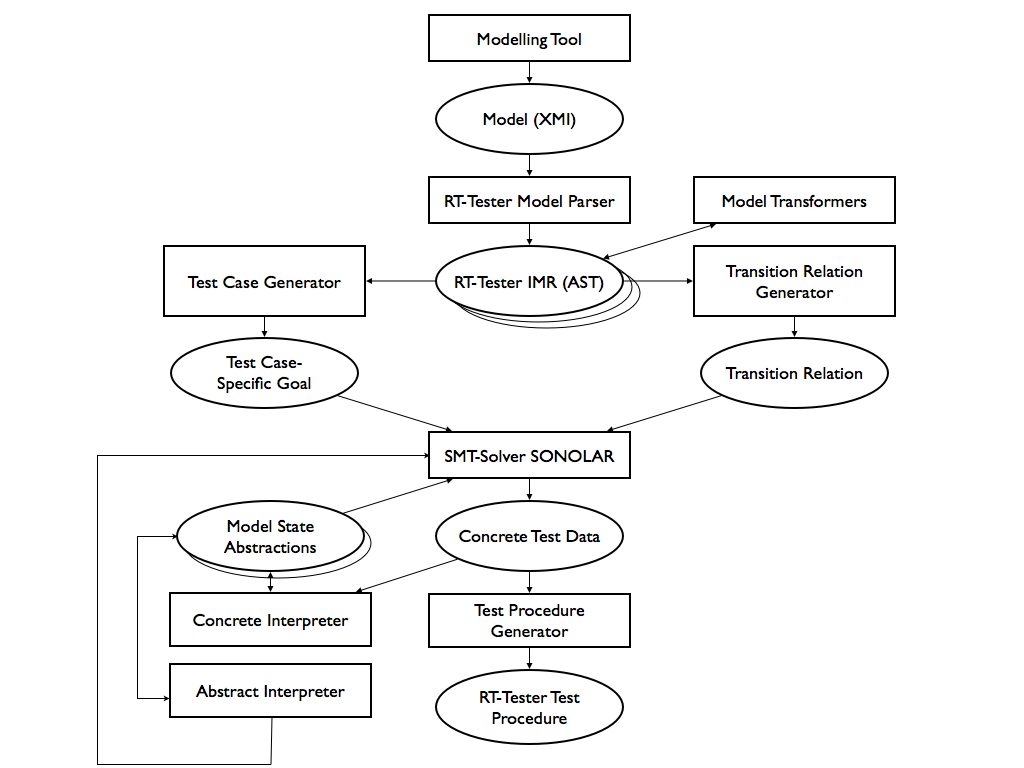
Figure 1: Components of the RT-Tester test case/test data generator.

The starting point for MBT is a concrete test model describing the expected behaviour of the system under test (SUT) and, optionally, the behaviour of the operational environment to be simulated in test executions by the testing environment (TE) (see Fig. 1). Models developed in a specific formalism are transformed into some textual representation supported by the modelling tool (usually XMI format). A model parser front-end reads the model text and creates an internal model representation (IMR) of the abstract syntax.

A transition relation generator creates the initial state and the transition relation of the model as an expression in propositional logic, referring to pre-and post-states. Model transformers create additional reduced, abstracted or equivalent model representations which are useful to speed up the test case and test data generation process.

A test case generator creates propositional formulas representing test cases built according to a given strategy. A satisfiability modulo theory (SMT) solver calculates solutions of the test case constraints in compliance with the transition relation. This results in concrete computation fragments yielding the time stamps and input vectors to be used in the test procedure implementing the test case (and possibly other test cases as well). An interpreter simulating the model in compliance with the transition relation is used to investigate concrete model executions continuing the computation fragments calculated by the SMT solver or, alternatively, creating new computations based on environment simulation and random data selection. An abstract interpreter supports the SMT solver in finding solutions faster by calculating the minimum number of transition steps required to reach the goal, and by restricting the ranges of inputs and other model variables for each state possibly leading to a solution. Finally, the test procedure generator creates executable test procedures as required by the test execution environment by mapping the computations derived before into time-controlled commands sending input data to the SUT and by creating test oracles from the SUT model portion checking SUT reactions on the fly, in dependency of the stimuli received before from the TE.

3 Modelling Aspects

3.1 Modelling Formalisms

It is our expectation that the ongoing discussions about suitable modelling formalisms for reactive systems – from UML via process algebras and synchronous languages to domain-specific languages – will not converge to a single preferred formalism in the near future. As a consequence it is important to separate the test case and test data generation algorithms from concrete modelling formalisms.

RT-Tester supports subsets of UML [25] and SysML [24] for creating test models: SUT structure is expressed by composite structure or block diagrams, and behaviour is specified by means of state machines and operations (a small SysML-based case study is presented Appendix A). The parser front end reads model exports from different tools in XMI format. Another parser reads Matlab/Simulink models. For software testing, a further front end parses transition graphs of C functions.

The first versions of RT-Tester supported CSP [36] as modelling language, but the process-algebraic presentation style was not accepted well by practitioners. Support for an alternative textual formalism is currently elaborated by creating a front-end for CML [44], the COMPASS modelling language specialised on systems of systems (SoS) design, verification and validation. In CML, the problems preventing a wider acceptance of CSP for test modelling have been removed.

Some formalisms are domain-specific and supported on customers’ request: in [22] automated MBT against a timed variant of Moore Automata is described, which is used for modelling control logic of level crossing systems.

3.2 A Sample Model

In Appendix A a case study is presented which will be used in this paper to illustrate modelling techniques, test case generation and requirements tracing. The case study models the turn indication and emergency flashing functions as present in modern vehicles. While this study is just a small simplified example, a full test model of the turn indication function as realised in Daimler Mercedes cars has been published in [27] and is available under http://www.mbt-benchmarks.org.

3.3 Semantic Models

In addition to the internal model representation which is capable of representing abstract syntax trees for a wide variety of formalisms, a semantic model is needed which is rich enough to encode the different behaviours of these formalisms. As will be described in Section 4, operational model semantics is the basis for automated test data generation, and it is also needed to specify the conformance relation between test model and SUT, which is checked by the tests oracles generated from the model (see below).

A wide variety of semantic models is available and suitable for test generation. Different variants of labelled transition systems (LTS) are used for testing against process algebraic models, like Hennessy’s acceptance tree semantics [15], the failures-divergence semantics of CSP (they come in several variants [31]) and Timed CSP [36], the LTS used in I/O conformance test theory [40, 41], or the Timed LTS used for the testing theory of Timed I/O Automata [38]. As an alternative to the LTS-based approach, Cavalcanti and Gaudel advocate for the Unifying Theories of Programming [16], that are used, for example, as a semantic basis for the Circus formalism and its testing theory [9], and for the COMPASS Modelling Language CML mentioned above.

For our research and MBT tool building foundations we have adopted Kripke Structures, mainly because our test generation techniques are close to techniques used in (bounded) model checking, and many fundamental results from that area are formulated in the semantic framework of Kripke Structures [11]. Recall that a Kripke Structure is a state transition system $K=(S,S_{0},R,L)$ with state space $S$, initial states $S_{0}\subseteq S$, transition relation $R\subseteq S\times S$ and labelling function $L:S\rightarrow\Pwr(AP)$ associating each state $s$ with the set $L(s)$ of atomic propositions $p\in AP$ which hold in this state. The behaviour of $K$ is expressed by the set of computations $\pi=s_{0}.s_{1}.s_{2}\ldots\in S^{\omega}$, that is, the infinite sequences $\pi$ of states fulfilling $s_{0}\in S_{0}$ and $R(s_{i},s_{i+1}),i=0,1,2,\ldots$. In contrast to LTS, Kripke Structures do not support a concept of events, these have to be modelled by propositions becoming true when changing from one state to a successor state. For testing purposes, states $s\in S$ are typically modelled by variable valuation functions $s:V\rightarrow D$ where $V$ is a set of variable symbols $x$ mapped by $s$ to their current value $s(x)$ in their appropriate domain (bool, int, float, …) which is a subset of $D$. The variable symbols are partitioned into $V=I\cup O\cup M$, where $I$ contains the input variables of the SUT, $O$ its output variables, and $M$ its internal model variables which cannot be observed during tests. Concurrency can be modelled both for the synchronous (“true parallelism”) [8] and the interleaving variants of semantics [11, Chapter 10]. Discrete or dense time can be encoded by means of a variable $\hat{t}$ denoting model execution time. For dense-time models this leads to state spaces of uncountable size, but the abstractions of the state space according to clock regions or clock zones, as known from Timed Automata [11] can be encoded by means of atomic propositions and lead to finite-state abstractions.

Observe that there should be no real controversy about whether LTS or Kripke Structures are more suitable for describing behavioural semantics of models: De Nicola and Vaandrager [23] have shown how to construct property-preserving transformations of LTS into Kripke Structures and vice versa.

3.4 Conformance Relations

Conformance relations specify the correctness properties of a SUT by comparing its actual behaviour observed during test executions to the possible behaviours specified by the model. A wide variety of conformance relations are known. For Mealy automata models, Chow used an input/output-based equivalence relation which amounted to isomorphism between minimal automata representing specification and implementation models [10]. in the domain of process algebras Hennessy and De Nicola introduced the relation of testing equivalence which related specification process behaviour to SUT process behaviour [12]. For Lotus, this concept was explored in depth by Brinksma [7], Peleska and Siegel showed that it could be equally well applied for CSP and its refinement relations [26], and Schneider extended these results to Timed CSP [35]. Tretmans introduced the concept of I/O conformance [40]. Vaandrager et. al. used bi-similarity as a testing relation between timed automata representing specification and implementation [38]. All these conformance relations have in common, that they are defined on the model semantics, that is, as relations between computations admissible for specification and implementation, respectively.

Conformance in the synchronous deterministic case.

For our Kripke structures, a simple variant of I/O conformance suffices for a surprisingly wide range of applications: for every trace $s_{0}.s_{1}\ldots s_{n}$ identified for test purposes in the model, the associated test execution trace $s_{0}^{\prime}.s_{1}^{\prime}\ldots s_{n}^{\prime}$ should have the same length and satisfy

$$\forall i\in\{0,\ldots,n\}:s_{i}|_{I\cup O\cup\{\hat{t}\}}=s_{i}^{\prime}|_{I\cup O\cup\{\hat{t}\}}$$

that is, the observable input and output values, as well as the time stamps should be identical.

This very simple notion of conformance is justified for the following scenarios of reactive systems testing: (1) The SUT is non-blocking on its input interfaces, (2) the most recent value passed along output interfaces can always be queried in the testing environment, (3) each concurrent component is deterministic, and (4) the synchronous concurrency semantics applies. At first glance, these conditions may seem rather restrictive, but there is a wide variety of practical test applications where they apply: many SUT never refuse inputs, since they communicate via shared variables, dual-ported ram, or non-blocking state-based protocols. Typical hardware-in-the-loop testing environments always keep the current output values of the SUT in memory for evaluation purposes, so that even message-based interfaces can be accessed as shared variables in memory (additionally, test events may be generated when an output message of the SUT actually arrives in the test environment (TE). For safety-critical applications the control decisions of each sequential sub-component of the SUT must be deterministic, so that the concept of may tests [15], where a test trace may or may not be refused by the SUT does not apply. As a consequence, the complexity and elegance of testing theories handling non-deterministic internal choice and associated refusal sets and unpredictable outputs of the SUT are not applicable for these types of systems. Finally, synchronous systems are widely used for local control applications, such as, for example, PLC controllers or computers adhering to the cyclic processing paradigm.

In RT-Tester this conformance relation is practically applied, for example, when testing software generated from SCADE models [13]: the SCADE tool and its modelling language adhere to the synchronous paradigm. The software operates in processing cycles. Each cycle starts with reading input data from global variables shared with the environment; this is followed by internal processing steps, and the output variables are updated at the end of the cycle. Time $\hat{t}$ is a discrete abstraction corresponding to a counter of processing cycles.

Conformance in presence of non-determinism.

For distributed control systems the synchronous paradigm obviously no longer applies, and though single sequential SUT components will usually still act in a deterministic way, their outputs will interleave non-deterministically with those of others executing in a concurrent way. Moreover, certain SUT outputs may change non-deterministically over a period of time, because the exact behavioural specification is unavailable. These aspects are supported in RT-Tester in the following ways.

• All SUT output interfaces $y$ are associated with (1) an acceptable deviation $\varepsilon_{y}$ from the accepted value (so any observed value $s^{\prime}(y)$ deviating from the expected value $s(y)$ by $|s^{\prime}(y)-s(y)|\leq\varepsilon$ is acceptable), (2) an admissible latency $\delta_{y}^{0}$ (so any observed value $s^{\prime}(y)$ for the expected value $s(y)$ is not timed out as long as $s^{\prime}(\hat{t})-s(\hat{t})\leq\delta_{y}^{0}$, and (3) an acceptable time $\delta_{y}^{1}$ for early changes of $y$ (so $s(\hat{t})-s^{\prime}(\hat{t})\leq\delta_{y}^{1}$ is still acceptable).

• A time-bounded non-deterministic assignment statement y = UNDEF(t,c) stating that $y$’s valuation is arbitrary for a duration of t time units, after which it should assume value c (with an admissible deviation and an admissible delay).

• A model transformation turning the SUT model into a test oracle: it

  • extends the variable space by one additional output variable $y^{\prime}$ per SUT output $y\in O$,

  • adds one concurrent checker component ${\cal O}_{y}$ per SUT output signal, operating on $y$ and $y^{\prime}$,

  • adds one concurrent component ${\cal P}$ processing the timed input output trace as observed during the test execution, with observed SUT outputs written to $y^{\prime}$ (instead of $y$),

  • transforms each concurrent SUT component $C_{i}$ into ${\cal C}_{i}$.

  This is described in more detail in the next paragraphs.

The transformed SUT components ${\cal C}_{i}$ operate as sketched in the example shown in Fig. 2. Every write of $C_{i}$ to some output $y$ is performed in ${\cal C}_{i}$ as well, ${\cal C}_{i}$ however, waits for the corresponding output value $y^{\prime}$ observed during test execution to change until it fits to the expected value of $y$ (guard condition $|y^{\prime}-y|\leq\varepsilon$). This helps to adjust to small admissible delays of in the expected change of $y^{\prime}$ observed in the test: the causal relation “$a$ is written after $y$ has been changed is preserved in this way. If $C_{i}$ uses another output $z$ (written, for example, by a concurrent component $C_{j}$) in a guard condition, it is replaced by variable $z^{\prime}$ containing the observed output during test execution. This helps to check for correctness of relative time distances like “output $w$ is written 10ms after $z$ has been changed”, if the actual output on $z^{\prime}$ is delayed by an admissible amount of time.

The concurrent test oracles ${\cal O}_{y}$ operate as shown in Fig. 3: If some component ${\cal C}_{i}$ writes to an expected output $y$, the oracle traverses into control state s2. If the corresponding observed output $y^{\prime}$ is also adjusted in ${\cal P}$, such that $|y^{\prime}-y|\leq\varepsilon_{y}$ holds before $\delta_{y}^{0}$ time units have elapsed, the change to $y^{\prime}$ is accepted and the oracle transits to s0. Otherwise the oracle transits into the error state. If the observed value changes unexpectedly above threshold $\varepsilon_{y}$, the oracle changes into location s3. If the expected value $y$ also changes shortly afterwards, this means that the SUT was just some admissible time earlier than expected according to the model, and the change is monitored via state s2 as before. If $y$, however, does not change for at least $\delta_{y}^{1}$ time units, we have uncovered an illegal output change of the SUT and transit into the error state.

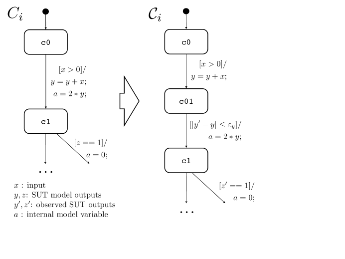
Figure 2: Example of original SUT component $C_{i}$ and transformed component ${\cal C}_{i}$.

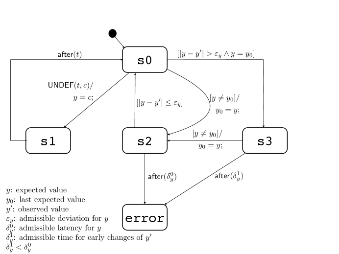
Figure 3: Test oracle component observing one SUT output interface $y$.

A test execution (that is, an input/output trace) performed with the SUT conforms to the model if and only if the transformed model accepts the test execution processed by ${\cal P}$ in the sense that none of the oracles transits into an error state. RT-Tester uses this conformance relation for hardware-in-the-loop system testing, as, for example, in the tests of the automotive controller network supporting the turn indication function in Daimler Mercedes vehicles [27].

3.5 Test-Modelling Related Challenges

With suitable test models available, test efficiency and test quality are improved in a considerable way. The elaboration of a model, however, can prove to be a major hurdle for the success of MBT in practice.

1. If complex models have to be completed before testing can start, this induces an unacceptable delay for the proper test executions.

2. For complex SUT, like systems of systems, test models need to abstract from a large amount of detail, because otherwise the resulting test model would become unmanageable.

3. The required skills for test engineers writing test models are significantly higher than for test engineers writing sequential test procedures.

We expect that problem 1 will be solved in the future by incremental model development, where test suites with increasing coverage and error detection capabilities can be run between model increments. The current methods based on sequential state machines as described by [42] may be extended to partially automated approaches where test model designers provide – apart from interface descriptions – initial architectural frames and suggestions for internal state variables, and automated machine learning takes these information into account. Furthermore, the explicit state machine construction may be complemented by incremental elaboration of transition relations: as pointed out by [28] for the purpose of test data generation, concurrent real-time models with complex state space are often better expressed by means of their transition relation than by explicit concurrent state machines. Promising attempts to construct test models in an incremental way from actual observations obtained during SUT simulations or experiments with the actual SUT indicate that test model development can profit from “re-engineering” SUT properties or model fragments from observations [30].

The problem of model complexity can be overcome by introducing contracts for the constituent systems of a large system of systems. This type of abstractions is investigated, for example, in the COMPASS project.

With respect to the third problem it is necessary to point out in management circles that competent testing requires the same skills as competent software development. So if modelling skills are required for model-driven software and system development, these skills are required for test engineers as well.

4 Requirements, Test Cases and Trustworthy Test Strategies

4.1 Requirements

If a test model has been elaborated in an adequate way, it will reflect the requirements to be tested. At first glance, however, it may not be obvious to identify the model portions contributing to a given requirement. Formally speaking, a requirement is reflected by certain computations $\pi=s_{0}.s_{1}.s_{2}\ldots$ of the model. Computations can be identified, for example, by some variant of temporal logic, and we use Linear Temporal Logic (LTL) [11, Chapter 3] for this purpose.

Consider, for example, requirement REQ-001 (Flashing requires sufficient voltage) from the sample application specified in Appendix A, Table 1. It can be readily expressed in LTL as

$$\mathbf{G}(\text{Voltage}\leq 80\Rightarrow\mathbf{X}(\neg(\text{FlashLeft}\vee\text{FlashRight})\ \mathbf{U}\ \text{Voltage}>80))$$ (1)

This is a black-box specification: it only refers to input and output interfaces of the SUT and is valid without any model. With a model at hand, however, the specification can be slightly simplified, because the relevant SUT reactions have been captured by state machine OUTPUT_CTRL (see Fig. 8).

$$\mathbf{G}(\text{Voltage}\leq 80\Rightarrow\mathbf{X}(\text{Idle}\ \mathbf{U}\ \text{Voltage}>80))$$

In control state Idle the indication lights are never activated. Now the computations contributing to REQ-001 are exactly the ones finally fulfilling the premise $\text{Voltage}\leq 80$, where the effect of the requirement may become visible, that is,

$$\mathbf{F}(\text{Voltage}\leq 80)$$

It is unnecessary to specify the effects of the requirement in this formula, because we are only considering valid model computations, and the effect is encoded in the model.

Observe that the application of LTL to characterise model computations associated with a requirement differs from its utilisation for black-box specification as in formula (1), where the behaviour required along those computations has to be specified in the formula, and only interface variables of the system may be referenced. It also differs from the application of temporal logics in property checking, where either all (a required property) or no computations (a requirements violation) of the model should fulfil the formula.

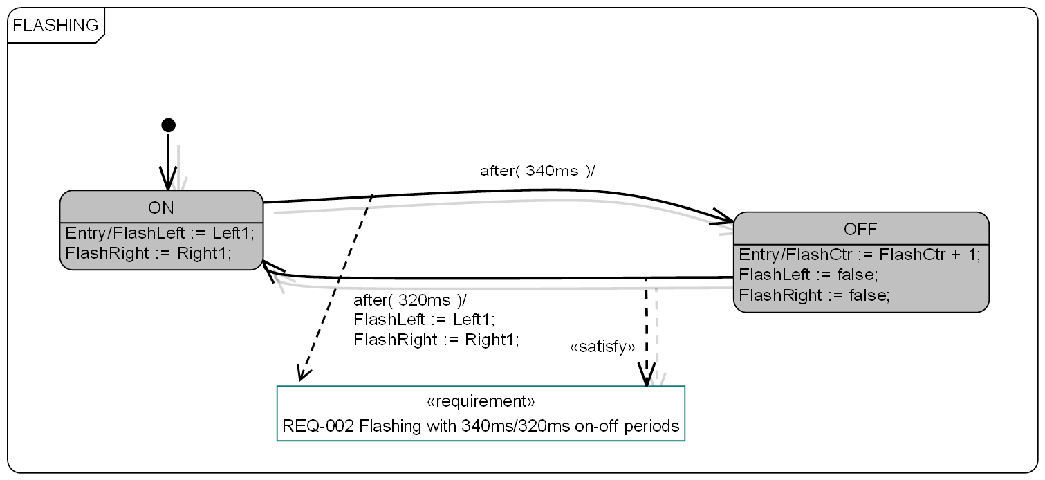
Figure 9: Decomposition of control state FLASHING.

Referring to internal model elements frequently simplifies the formulas for characterising computations. Requirement REQ-002 (Flashing with 340ms/320ms on-off periods), for example, is witnessed by all computations satisfying (see Fig.9)

$$\mathbf{F}(\text{OFF}\wedge\mathbf{X}\text{ON})$$ (2)

4.2 Requirements Tracing to the Model

The SysML modelling formalism [24] provides syntactic means to identify requirements in the model. In Fig.9, for example, the transitions $\text{ON}\rightarrow\text{OFF}$ and $\text{OFF}\rightarrow\text{ON}$ realise the flashing period specified by REQ-002. This is documented by means of the «satisfy» relation drawn from the transitions to the requirement. The interpretation of this relation is that every model computation finally covering one of the two transitions or both contributes to the requirement. Since computations cover $\text{OFF}\rightarrow\text{ON}$ if and only if they fulfil $\mathbf{F}(\text{OFF}\wedge\mathbf{X}\text{ON})$, the «satisfy» relation from $\text{ON}\rightarrow\text{OFF}$ to REQ-002 is redundant. Other examples for such simple relationships between model elements an requirements are shown in the state machine depicted in Fig 7. Formally speaking, these simple relationships are of the type

$$\mathbf{F}\langle\text{State Formula}\rangle$$ (3)

where the state formula expresses the condition that a model element related to the requirement is covered: for REQ-002, the formula (2) can be expressed in the form (3) as

$$\mathbf{F}(\text{OFF}\wedge(\hat{t}-t_{\text{OFF}})\geq 320$$

Here $t_{\text{OFF}}$ denotes the timer variable that stores the current time whenever control state OFF is entered and $\hat{t}$ is the current model execution time, so $(\hat{t}-t_{\text{OFF}})$ expresses the fact that the relative time event $\text{after}(320ms)$ has occurred. In this case the transition $\text{OFF}\rightarrow\text{ON}$ must be taken, since UML/SysML state machine priority assigns higher priority to lower-level transitions: even if transitions $\text{FLASHING}\rightarrow\text{FLASHING}$ or $\text{FLASHING}\rightarrow\text{Idle}$ of the state machine in Fig. 8 are enabled, transition $\text{OFF}\rightarrow\text{ON}$ has higher priority because it resides in the sub-maschine of FLASHING.

Evaluations of system requirements in the automotive domain (in cooperation with Daimler) have shown that approximately 80% of requirements are reflected by model computations satisfying

$$\mathbf{F}\left(\bigvee_{i=0}^{h}\phi_{i}\right)$$

where the $\phi_{i}$ are state formulas, each one expressing coverage of a single model element.

About 20% of system requirements require more complex witnesses, whose LTL specification involve nested path operators and state formulas referring to model elements, variable valuations and time. For these situations, we use constraints containing the more complex LTL formulas, and the constraints are linked to their associated requirements by means of the «satisfy» relation. Table 2 lists the requirements of the case study captured in Table 1, and associates the constraints characterising the witness traces for each requirement.

4.3 Test Cases

Since tests must terminate after a finite number of steps, they consist of traces $\iota=s_{0}\ldots s_{k}$ probing prefixes of relevant model computations $\pi=s_{0}\ldots s_{k}.s_{k+1}\ldots$. If $\pi$ is a witness for some requirement R characterised by LTL formula $\phi$, a suitable test case $\iota$ has to be constructed in a way that at least does not violate $\phi$ while transiting through states $s_{0}\ldots s_{k}$, even though $\phi$ will be violated by many possible extensions of $\iota$. This problem is well-understood from the field of bounded model checking (BMC), and Biere et. al. [4, 5] introduced a step semantics for evaluating LTL formulas on finite model traces. To this end, expression $\langle\varphi\rangle_{i}^{k-i}$ states that formula $\varphi$ holds in state $s_{i}$ of a trace of length $k+1$. For the operators of LTL, their semantics can then be specified inductively by

• $\langle\mathbf{G}~{}\varphi\rangle_{0}^{k}=\bigwedge_{i=0}^{k}\langle\varphi\rangle_{i}^{k-i}$    ($\mathbf{G}\phi$ is not violated on $\iota=s_{0}\ldots s_{k}$)

• $\langle\mathbf{X}~{}\varphi\rangle_{i}^{k-i}=\langle\varphi\rangle_{i+1}^{k-i-1}$

• $\langle\varphi~{}\mathbf{U}~{}\psi\rangle_{i}^{k-i}=\langle\psi\rangle_{i}^{k-i}\vee(\langle\varphi\rangle_{i}^{k-i}\wedge\langle\varphi~{}\mathbf{U}~{}\psi\rangle_{i+1}^{k-i-1})$,     $\langle\mathbf{F}\psi\rangle_{i}^{k-i}=\langle\mbox{{\tt true}}~{}\mathbf{U}~{}\psi\rangle_{i}^{k-i}$

Using this bounded step semantics, each LTL formula can be transformed into formulas of the type

$$tc\equiv J(s_{0})\wedge\bigwedge_{i=0}^{n}\Phi(s_{i},s_{i+1})\wedge G(s_{0},\ldots,s_{n+1})$$ (4)

which we call symbolic test cases and which can be handled by the SMT solver. Conjunct $J(s_{0})$ characterises the current model state $s_{0}$ from where the next test objective represented by some LTL formula $\phi$ should be covered. This formula has to be translated into a predicate $G(s_{0},\ldots,s_{n+1})$, using the semantic rules listed above. Predicate $\Phi$ is the transition relation of the model, and conjunct $\bigwedge_{i=0}^{n}\Phi(s_{i},s_{i+1})$ ensures that the solution of $G(s_{0},\ldots,s_{n+1})$ results in a valid trace of the model, starting from $s_{0}$.

Example 4.1.

ex:ltl Consider LTL formula

$$\phi\equiv(x=0)\mathbf{U}(y>0\wedge\mathbf{X}(\mathbf{G}z=1))$$

and suppose we are looking for a witness trace $\iota=s_{0}\ldots s_{n}\ldots$ with a length of at least $n+1$ or longer. Then the SMT solver is activated with the following BMC instances to solve.

In step 0, try solving

$$bmc_{0}\equiv\left(\bigwedge_{i=0}^{n}\Phi(s_{i},s_{i+1})\right)\wedge s_{0}(y)>0\wedge\left(\bigwedge_{i=1}^{n+1}s_{i}(z)=1\right)$$

If this succeeds we are done: the solution of $bmc_{0}$ is a legal trace $\iota$ of the model, since $\Phi(s_{i},s_{i+1})$ holds for each pair of consecutive states in $\iota$. Formula $\phi$ holds on $\iota$ because $y>0$ is true in $s_{0}$ and $z=1$ holds for states $s_{1}\ldots s_{n+1}$, so the right-hand side operand of $\mathbf{U}$ is fulfilled in the initial state of this trace.

Otherwise we try to get a witness for the following formula in step 1.

$$bmc_{1}\equiv\left(\bigwedge_{i=0}^{n}\Phi(s_{i},s_{i+1})\right)\wedge s_{0}(x)=0\wedge s_{1}(y)>0\wedge\left(\bigwedge_{i=2}^{n+1}s_{i}(z)=1\right)$$

If no solution exists we continue with step 2.

$$bmc_{2}\equiv\left(\bigwedge_{i=0}^{n}\Phi(s_{i},s_{i+1})\right)\wedge s_{0}(x)=0\wedge s_{1}(x)=0\wedge s_{2}(y)>0\wedge\left(\bigwedge_{i=3}^{n+1}s_{i}(z)=1\right)$$

and so on, until a solution is found or no solution of length $n+1$ is feasible.

While LTL formulas are well-suited to specify computations fulfilling a wide variety of constraints, it has to be noted that it is also capable of defining properties of computations that will never be tested in practice, because they can only be verified on infinite computations and not on finite trace prefixes thereof (e.g., fairness properties). It is therefore desirable to identify a subset of LTL formulas that are tailored to the testers’ needs for specifying finite traces with certain properties. This subset is called SafetyLTL and has been introduced in [37]. It is suitable for defining safety properties of computations, that is, properties that can always be falsified on a finite computation prefix. The SafetyLTL subset of LTL can be syntactically characterised as follows.

• Negation is only allowed before atomic propositions (so-called negation normal form).

• Disjunction $\vee$ and conjunction $\wedge$ are always allowed.

• Next operators $\mathbf{X}$, globally operators $\mathbf{G}$ and weakly-until operators $\mathbf{W}$ are allowed.

• Semantically equivalent formulas also belong to SafetyLTL.

Concrete test data is created by solving constraints of the type displayed in Equation (4) using the integrated SMT solver SONOLAR [28]. Finally the test procedure generator takes the solutions calculated by the SMT solver and turns them into stimulation sequences, that is, timed input traces to the SUT. Moreover, the test procedure generator creates test oracles from the model components describing the SUT behaviour.

In requirements-driven testing, $G(s_{0},\ldots,s_{n+1})$ specifies traces that are witnesses of a certain requirement R. Indeed, Formula (4) specifies an equivalence class of traces that are suitable for testing R. In model-driven testing, $G(s_{0},\ldots,s_{n+1})$ specifies traces that are suitable for covering certain portions (control states, transitions, interfaces, …) of the model. In the paragraphs below it will be explained how requirements-driven and model-driven testing are related to each other.

4.4 Model Coverage Test Cases

Since adequate test models express all SUT requirements to be tested, it is reasonable to specify and perform test cases achieving model coverage. As we have seen above, a behavioural model element (state machine control state, transition, operation, …) is covered by a trace $\iota=s_{0}\ldots s_{k}$, if the element’s behaviour is exercised during some transition $s_{i}\rightarrow s_{i+1}$. For a control state $c$ this means that $s_{i+1}(c)=\mbox{{\tt true}}$, and, consequently, the state’s entry action (if any) is executed. For a transition this means that its firing condition becomes true in some $s_{i}$. Operations $f$ are covered when they are associated with actions of covered states or transitions executing $f$.

There exists a wide variety of model coverage strategies, many of them are discussed in [43]. The standards for safety-critical systems development and V&V have only recently started to consider the model-driven development and V&V paradigm. It seems that the avionic standard RTCA DO-178C [33] is currently the most advanced with respect to model-based systems engineering. It requires to achieve operation coverage, transition coverage, decision coverage, and equivalence class and boundary value coverage, when verifying design models [32, Table MB.6-1]. Neither the standard, nor [43], however, elaborate on coverage of timing conditions (e.g., clock zones in Time Automata) or the coverage of execution state vectors of concurrent model components.

In RT-Tester, the following model coverage criteria are currently implemented: (1) basic control state coverage, (2) transition coverage, MC/DC coverage, (3) hierarchic transition coverage with or without MC/DC coverage, (4) equivalence class and boundary value coverage, (5) basic control state pairs coverage, (6) interface coverage and (7) block coverage.

Basic control state pairs coverage exercises all feasible control state combinations of concurrent state machines in writer-reader relationship. The equivalence class coverage technique in combination with basic control state pairs coverage also produces a (not necessarily complete) coverage of clock zones.

Each of these coverage criteria can be specified by means of LTL formulas or, equivalently, BMC instances.

Example 4.2.

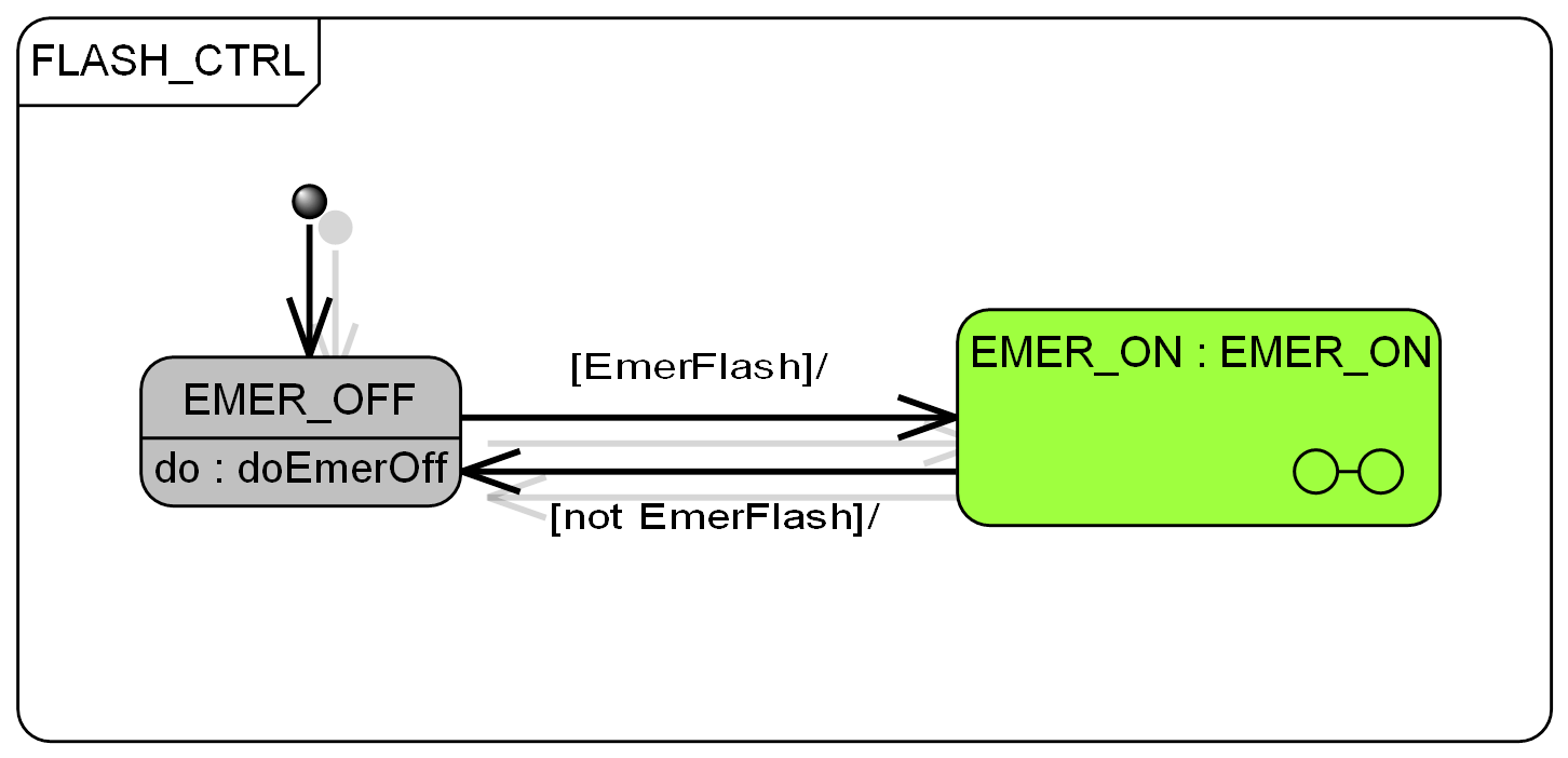
Figure 6: State machine controlling left/right and emergency flashing.

ex:cspairs For state machine FLASH_CTRL (Fig. 6), the hierarchic transition coverage is achieved by test cases

$$tc_{1} \equiv \mathbf{F}(\text{EMER\_OFF}\wedge\text{EmerFlash})$$

$$tc_{2} \equiv \mathbf{F}(\text{EMER\_ACTIVE}\wedge\text{TurnIndLvr}\neq 0\wedge{}$$

$$((\text{TurnIndLvr}=1)\neq\text{Left1}\vee(\text{TurnIndLvr}=2)\neq\text{Right1}))$$

$$tc_{3} \equiv \mathbf{F}(\text{EMER\_ACTIVE}\wedge(\text{Left1}\vee\text{Right1})\wedge\text{TurnIndLvr}=0)$$

$$tc_{4} \equiv \mathbf{F}(\text{TURN\_IND\_OVERRIDE}\wedge\text{TurnIndLvr}=0)$$

$$tc_{5} \equiv \mathbf{F}(\neg\text{EmerFlash}\wedge\text{EMER\_ACTIVE}\wedge{}$$

$$((\text{TurnIndLvr}\neq 0\wedge\text{TurnIndLvr}=\text{Left1}\vee\text{TurnIndLvr}=\text{Right1})\vee{}$$

$$(\text{TurnIndLvr}=0\wedge\neg(\text{Left1}\vee\text{Right1})))$$

$$tc_{6} \equiv \mathbf{F}(\neg\text{EmerFlash}\wedge\text{TURN\_IND\_OVERRIDE}\wedge\text{TurnIndLvr}\neq 0)$$

4.5 Automated Compilation of Traceability Data

Having identified the test cases suitable for model coverage, these can be related to requirements in an automated way.

• If requirement R is linked to model elements by «satisfy» relationships, then the test cases covering these elements are automatically related to R.

• If requirement R is characterised by a LTL formula $\phi$ not directly related to model elements, we proceed as follows.

  • Transform $\phi$ into disjunctive normal form $\phi\equiv\bigvee_{i=0}^{m}\phi_{i}$ and associate test cases for each $\phi_{i}$ separately.

  • Each test case $tc\equiv\psi$ derived from the model is related to R, if $\psi\Rightarrow\phi_{i}$ holds.

  • If test case $tc\equiv\psi$ is neither stronger nor weaker than the requirement in the sense that $\psi\wedge\phi_{i}$ has a solution, add a new test case $tc^{\prime}\equiv\psi\wedge\phi_{i}$ and relate $tc^{\prime}$ to R.

  • If at least one of two test cases $tc_{1}\equiv\mathbf{F}\psi_{1}$ and $tc_{2}\equiv\mathbf{F}\psi_{2}$ implies the requirement and $tc^{\prime}\equiv\mathbf{F}(\psi_{1}\wedge\psi_{2})$ has a solution, add $tc^{\prime}$ to the test case database and trace it to R.

Example 4.3.

ex:tcreqtrace Consider requirement REQ-002 (Flashing with 340ms/320ms on-off periods) of the example from Table 1. It is characterised by covering transitions $\text{ON}\rightarrow\text{OFF}$ and $\text{OFF}\rightarrow\text{ON}$ (see Table 2). By tracing these transitions back to model coverage test cases, the following cases can be identified, and these trace back to REQ-002.

$$tc_{7} \equiv \mathbf{F}(\text{OFF}\wedge(\hat{t}-t_{\text{OFF}})\geq 320)$$

$$tc_{8} \equiv \mathbf{F}(\text{OFF}\wedge(\hat{t}-t_{\text{OFF}})\geq 320\wedge\text{TurnIndLvr}=1)$$

$$tc_{9} \equiv \mathbf{F}(\text{OFF}\wedge(\hat{t}-t_{\text{OFF}})\geq 320\wedge\text{TurnIndLvr}=2)$$

$$tc_{10} \equiv \mathbf{F}(\text{OFF}\wedge(\hat{t}-t_{\text{OFF}})\geq 320\wedge\text{EMER\_ACTIVE})$$

$$tc_{11} \equiv \mathbf{F}(\text{OFF}\wedge(\hat{t}-t_{\text{OFF}})\geq 320\wedge\text{TURN\_IND\_OVERRIDE})$$

The test cases listed here are only a subset of the complete list that traces back to REQ-002. Test cases $tc_{8},tc_{9}$ result from combining interface coverage on SUT input TurnIndLvr with coverage of the $\text{OFF}\rightarrow\text{ON}$. Cases $tc_{10},tc_{11}$ result from combining basic control state pairs coverage with the transition coverage. Test case $tc_{7}$ is redundant if any of the others is performed. It is quite obvious that the test case generation technique defined above runs into combinatorial explosion problems. Even for the small sample system discussed here, the list of test cases from Example LABEL:ex:tcreqtrace could be extended by

$$tc_{12} \equiv \mathbf{F}(\text{OFF}\wedge(\hat{t}-t_{\text{OFF}})\geq 320\wedge\text{EMER\_ACTIVE}\wedge\text{TurnIndLvr}=0)$$

$$tc_{13} \equiv \mathbf{F}(\text{OFF}\wedge(\hat{t}-t_{\text{OFF}})\geq 320\wedge\text{EMER\_ACTIVE}\wedge\text{TurnIndLvr}=1)$$

$$tc_{14} \equiv \mathbf{F}(\text{OFF}\wedge(\hat{t}-t_{\text{OFF}})\geq 320\wedge\text{EMER\_ACTIVE}\wedge\text{TurnIndLvr}=2)$$

$$\ldots$$

4.6 Test Case Selection According to Criticality

It is quite obvious that the number of test cases related to a requirement can become quite vast, and that some of the test cases investigate more specific situations than others. This problem is closely related to the problem of exhaustive testing which will be discussed below. Since an exhaustive execution of all test case combinations related to a requirement will be impossible for fair-sized systems, a justified reduction of the potentially applicable test cases to a smaller collection is required. In the case of safety-critical systems development, such a justification should conform to the standards applicable for V&V of these systems.

In the case of avionic systems, the RTCA DO-178C standard [33] requires structural tests with respect to data and control coupling and full requirements coverage through testing, but does not specify when a requirement has been verified with a sufficient number of test cases. Instead, the standard gives test end criteria by setting code coverage goals, the coverage to be achieved depending on the SUT’s criticality [32, MB.C-7]: for assurance level 1 systems (highest criticality), MC/DC coverage has to be achieved, for level 2 decision coverage, and for level 3 statement coverage. For levels 4 and 5, only high-level requirements have to be covered without setting any code coverage goals, and for assurance level 5 the requirement to test data and control coupling is dropped.

As a consequence, the model-based test case coverage can be tuned according to the code coverage achieved, whenever the source code is available and the assurance level is in 1 — 3: start with basic control state coverage cases related to the requirement, increase coverage by adding hierarchic and MC/DC coverage test cases until the required code coverage is achieved. Add interface and basic control state pairs coverage cases until the data and control coupling coverage has been achieved as well. For levels 4 or 5, no discussion is necessary, since here any “reasonable” test case assignment to each high-level requirement is acceptable, due to the low criticality of the SUT.

When MBT is applied on system level, however, it will generally be infeasible to measure code coverage achieved during system tests. For systems of systems, in particular, system-level tests will never cover any significant amount of code coverage, and the coverage values achieved will not be obtainable in most cases, both for technical and for security reasons. Here we suggest to proceed as follows.

• For assurance level 3, exercise

  • interface tests – this ensures verification of data and control coupling,

  • basic control state coverage test cases,

  • refine these test cases $tc\equiv\psi$ only if requirements have stricter characterisations $\phi_{i}$; in this case add $tc^{\prime}\equiv\psi\wedge\phi_{i}$.

• For assurance level 2, follow the same pattern, but use transition coverage test cases.

• For assurance level 1, exercise

  • interface tests,

  • basic control state pairs coverage test cases to refine the data and control coupling tests (recall that these test cases stem from writer-reader analyses),

  • MC/DC coverage test cases in combination with hierarchic transition coverage,

  • first-level refinements of test cases related to requirements as illustrated in Example LABEL:ex:tcreqtrace,

  • second level refinements (as in test cases $tc_{12},tc_{13},tc_{14}$ above), if the additional conjuncts have direct impact on the requirement.

Following these rules, and supposing that our sample system were of assurance level 1, the test cases displayed in Example LABEL:ex:tcreqtrace would be necessary. Test cases $tc_{12},tc_{13},tc_{14}$, however, would not be required, since the TurnIndLvr has no impact on REQ-002 according to the model: the risk of a hidden impact of this interface on the requirement has already been taken into account when testing $tc_{8},tc_{9}$.

4.6.1 Test Strategies Proving Conformance

An alternative for justifying test strategies consists in proving that they will finally converge to an exhaustive test suite establishing some conformance relation between model and SUT. This approach has a long tradition: one of the first contributions in this field was Chow’s W-Method [10] applicable for minimal state machines, which was generalised and extended into many directions, so that even in the core of the exhaustive test strategy for timed automata [38] some argument from the W-Method is used.

Though execution of exhaustive test suites will generally be infeasible in practice, convergence to exhaustive test suites ensures that new test cases added to the suite will really increase the assurance level by a positive amount: intuitively designed test strategies often do not possess this property, because additional test cases may just re-test SUT aspects already covered by existing ones.

The known exhaustive strategies typically operate on finite data types (discrete events, or variables with data ranges that can easily be enumerated). It is an interesting research challenge whether similar results can be obtained in presence of large data types, if application of equivalence class partitioning is justified. In [14] the authors formalise the concept of equivalence class partitioning and prove that exhaustive suites can be constructed for white-box test situations. In [19] this approach is currently generalised within the COMPASS project with respect to black-box testing and semantic models that are more general than the one underlying the results presented in [14].

4.7 Challenges to Test Case Generation and Test Strategy Design

The size of SoS state spaces implies that exhaustive investigation of the complete concrete state space will certainly be infeasible. We suggest to tackle this problem by two orthogonal strategies, as is currently investigated in the COMPASS project [18].

• On constituent system level, different behaviours associated with the same local mission threads will be comprised in equivalence classes. This reduces the complexity problem for SoS system testing to covering combinations of classes of constituent system behaviours instead of sequences of concrete state vector combinations.

• On SoS system level, “relevant” class combinations are identified by means of different variants of impact analysis, such as data flow analyses or investigation of contractual dependencies. Behaviours of constituent systems which do not affect the relevant class combinations under consideration will be selected according to the principle of orthogonal arrays [29], because this promises an effective combinatorial distribution of unrelated behaviours exercised concurrently with the critical ones.

Apart from size and complexity, SoS present another challenge, because they typically change their configuration dynamically during run-time. The dynamic adaptation of test objectives is particularly relevant for run-time acceptance testing of changing SoS configurations. In contrast to development models for SoS, however, we only have to consider bounded changes of SoS configurations, because every test suite can only consider a bounded number of configurations anyway. It remains to investigate how to determine configurations possessing sufficient error detection strength. Results from the field of mutation testing will help to determine this strength in a systematic and measurable way.

A further problem for systems of SoS complexity is presented by the fact that not every behaviour can be full captured in the model, which results in under-specification and non-determinism. Test strategy elaboration in presence of this problem be achieved in the following way.

• The SoS system behaviour is structured into several top-level operational modes. It is expected that switching between these modes can be performed in a deterministic way for normal behaviour tests: it is unlikely that SoS performing operational mode changes only on a random basis are acceptable and “testworthy”.

• Entry into failure modes is non-deterministic, but can be initiated in a deterministic way for test purposes by means of pre-planned failure injections.

• The behaviour in each operational mode is not completely deterministic, but can be captured by sets of constraints governing the acceptable computations in each mode. Test oracles will therefore no longer check for explicit output traces of the SUT but for compliance of the traces observed with the constraints applicable in each mode.

• For test stimulation purposes the SMT solver computes sequences of feasible mode switches and the test data provoking these switches.

• Incremental test model elaboration can be performed by adding constraints identified during test observations to the modes where they are applicable. To this end, techniques from machine learning seem to be promising.

Justification of test strategies will be performed by proving that they will “converge” to exhaustive tests proving some compliance relation between SUT and reference model.

5 Conclusion

In this article several aspects of industrial-strength model-based testing and its underlying methods have been presented. A reference tool has been described, so that the presentation may serve as a benchmark for alternative tools capable of handling test campaigns of equal or even higher complexity. Readers are invited to join the discussion on suitable benchmarks for MBT tools – initial suggestions on benchmarking can be found in [27] – and to contribute case studies and models to the MBT benchmark website http://www.mbt-benchmarks.org.

A further topic beyond the scope of this paper is of considerable importance for tool builders: MBT tools automating test campaigns for safety-relevant systems have to be qualified, and standards like RTCA DO-178C [33] for the avionic domain, CENELEC EN650128 [39] for the railway domain, and ISO 26262 [20] for the automotive domain have rather precise policies about how tool qualification can be obtained. A detailed comparison between tool qualification requirements of these standards is presented in [17], and it is described in [6] how tool qualification has been obtained for RT-Tester. We believe that the complexity of the algorithms required in MBT tools justifies that effort is spent on their qualification, so that their automated application will not mask errors of the SUT due to undetected failures in the tool.

Acknowledgements.

The author would like to thank the organisers of the MBT 2013 for giving him the opportunity to present the ideas summarised in this paper. Special thanks go to Jörg Brauer, Elena Gorbachuk, Wen-ling Huang, Florian Lapschies and Uwe Schulze for contributing to the results presented here.

Appendix A Case Study: Turn Indication Control Function

As a case study we consider the turn indication function of a vehicle providing left/right indication and emergency flashing by means of exterior lights flashing with a given frequency. Left/right indication is switched on by means of the turn indicator lever with its positions 0 (neutral), 1 (left), and 2(right). Emergency flashing is controlled by means of a switch with positions 0 (off) and 1 (on). Activating the indication lights is subject to the condition that the available voltage is sufficiently high. The requirements for the turn indication function are as shown in Table 1.

Table 1: Requirements of the turn indication control system

Requirement	Description
REQ-001 Flashing requires sufficient voltage	Indication lights are only active, if the electrical voltage (input Voltage) is $>80\%$ of the nominal voltage.
REQ-002 Flashing with 340ms/320ms on-off periods	If any lights are flashing, this is done synchronously with a 340ms ON – 320ms OFF period.
REQ-003 Switch on turn indication left	An input change from turn indication lever state TurnIndLvr = 0 or 2 to TurnIndLvr = 1 switches indication lights left (output FlashLeft) into flashing mode and switches indication lights right (output FlashRight) off.
REQ-004 Switch on turn indication right	An input change from turn indication lever state TurnIndLvr = 0 or 1 to TurnIndLvr = 2 switches indication lights right (output FlashRight) into flashing mode and switches indication lights left (output FlashLeft) off.
REQ-005 Emergency flashing on overrides left/right flashing	An input change from EmerFlash = 0 to EmerFlash = 1 switches indication lights left (output FlashLeft) and right (output FlashRight) into flashing mode, regardless of any previously activated turn indication.
REQ-006 Left-/right flashing overrides emergency flashing	Activation of the turn indication left or right overrides emergency flashing, if the latter has been activated before.
REQ-007 Resume emergency flashing	If turn indication left or right is switched off and emergency flashing is still active, emergency flashing is continued or resumed, respectively.
REQ-008 Resume turn indication flashing	If emergency flashing is turned off and turn indication left or right is still active, the turn indication is continued or resumed, respectively.
REQ-009 Tip flashing	If turn indication left or right is switched off before three flashing periods have elapsed, the turn indication will continue until three on-off periods have been performed.

The SysML test model for this system structured into TE and SUT blocks, as shown in Fig. 4. The interfaces shown in this diagram are the observable SUT outputs and writable inputs that may be accessed by the TE. RT-Tester allows for SysML properties and signal events to be exchanged between SUT and TE model components. The tool provides interface modules mapping their valuations onto concrete software or hardware interfaces and vice versa. In a software integration test the turn indication lever values and the status of the emergency switch may be passed to the SUT, for example, by means of shared variables. The SUT outputs (left-hand side lamps on/off, right-hand side lamps on/off) can also be represented by Boolean output variables of the SUT. In a HW/SW integration test interface modules would map the turn indication lever status and the emergency flash button to discrete inputs to the SUT. In a system integration test the actual voltage and the current placed by the SUT on the indication lamps would be measured. The interface abstraction required for the test level is specified by a signal map that associates abstract SysML model interfaces with concrete interfaces of the test equipment.

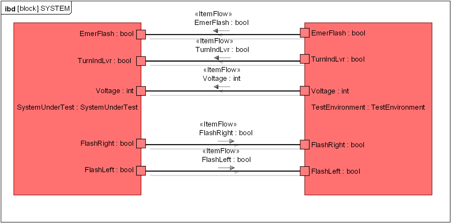
Figure 4: Interface between TE and SUT.

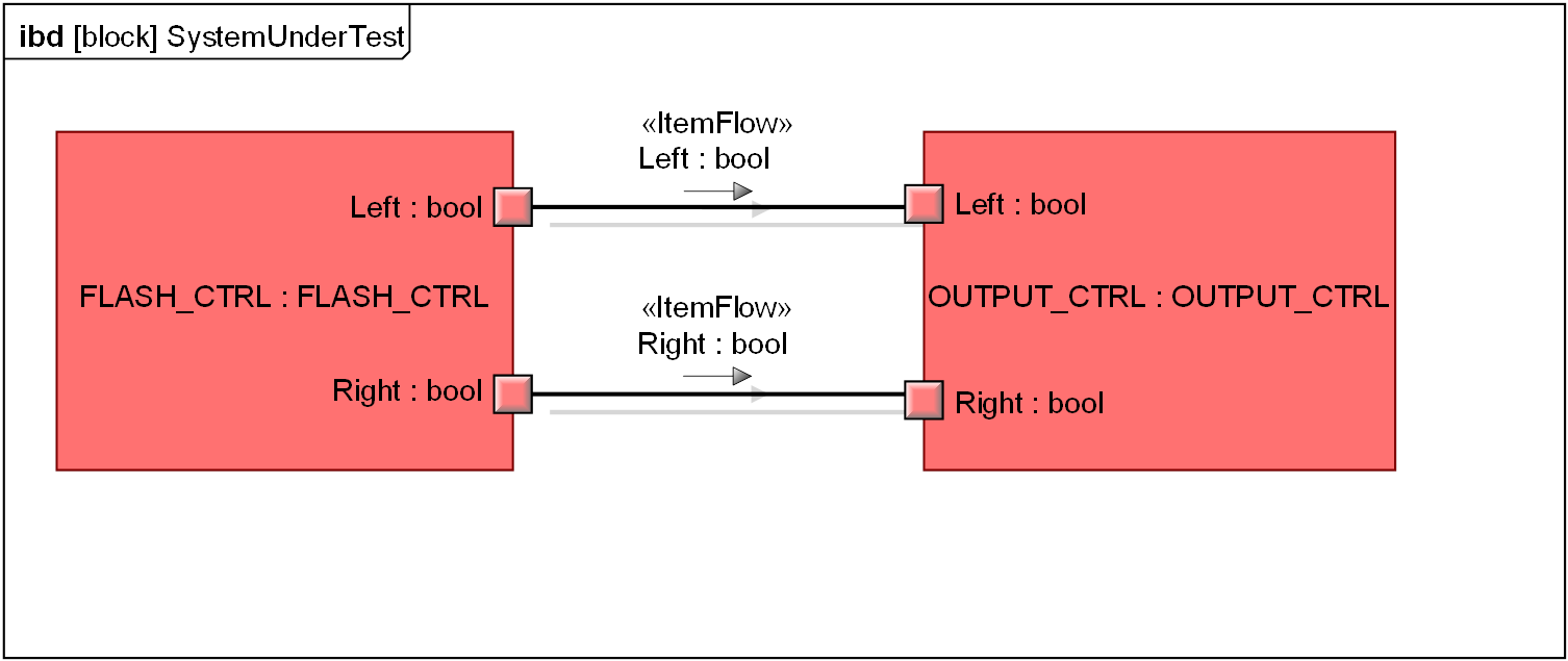
Figure 5: Functional decomposition of the SUT.

The structural view on the SUT has to be decomposed further, until each block is associated with a sequential behaviour. For the case study discussed here, the SUT is further decomposed into two concurrent functions as depicted in Fig. 5. Functional component FLASH_CTRL performs the decisions about left/right indication or emergency flashing. The decision is communicated to component OUTPUT_CTRL by means of internal interface Left (flashing on left-hand side indication lights if Left = 1) and Right (flashing on right-hand side indication lights if Right = 1). Block OUTPUT_CTRL controls the flashing cycles and switches off indication lamps if the voltage gets too low. The FLASH_CONTROL component operates as follows.

• As long as the emergency flash switch has not been activated, Left/Right are set according to the turn indication lever status. This is specified in do activity doEmerOff.

• As soon as the emergency flash switch EmerFlash is switched on, Left/Right are set as specified in sub-state machine EMER_ON (Fig 7).

• When entering EMER_ON, Left/Right are both set to true and the state machine remains in control state EMER_ACTIVE.

• When the turn indication lever is changed to left or right position, emergency flashing is overridden, and left/right indication is performed.

• Emergency flashing is resumed if the turn indication lever is switched into neutral position.

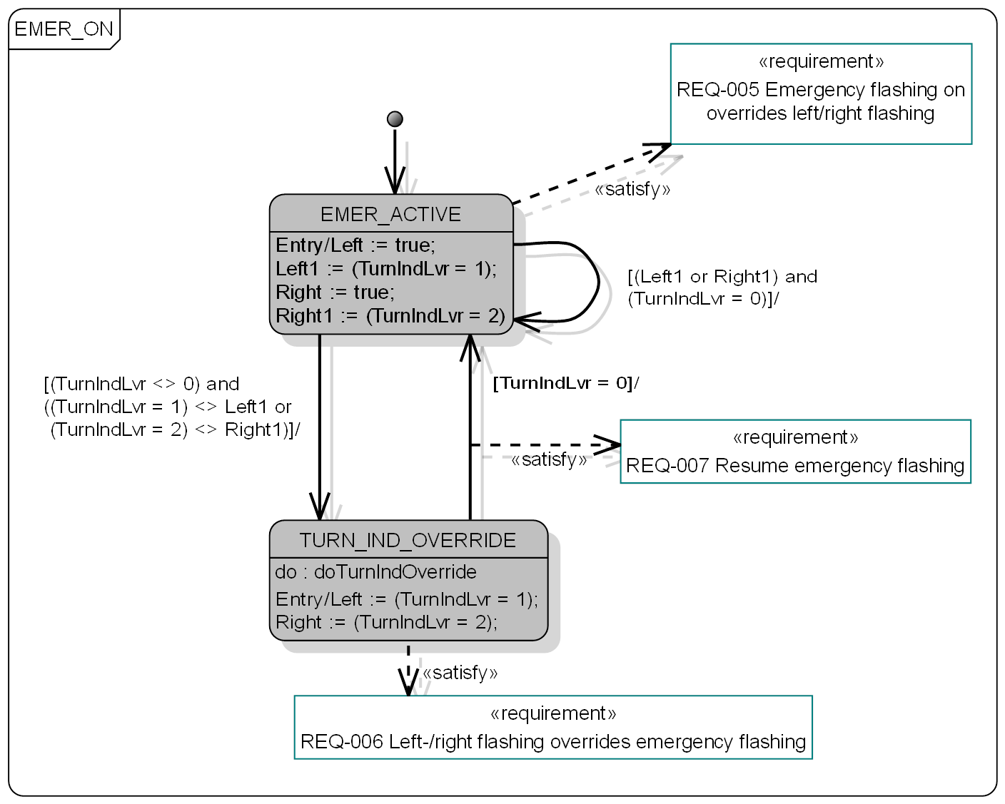
Figure 7: Decomposition of control state EMER_ON.

Function OUTPUT_CTRL sets the SUT output interfaces FlashLeft and FlashRight (Fig. 8 and 9). The indication lamps are switched according to the internal interface state Left/Right, if the voltage is greater than 80% of the nominal voltage. After the lamps have been on for 340ms, they are switched off and stay so until 320ms have passed. A counter FlashCtr is maintained: if the turn indication lever is switched from left or right back to the neutral position before 3 flashing periods have been performed, left/right indication will remain active until the end of these 3 periods.

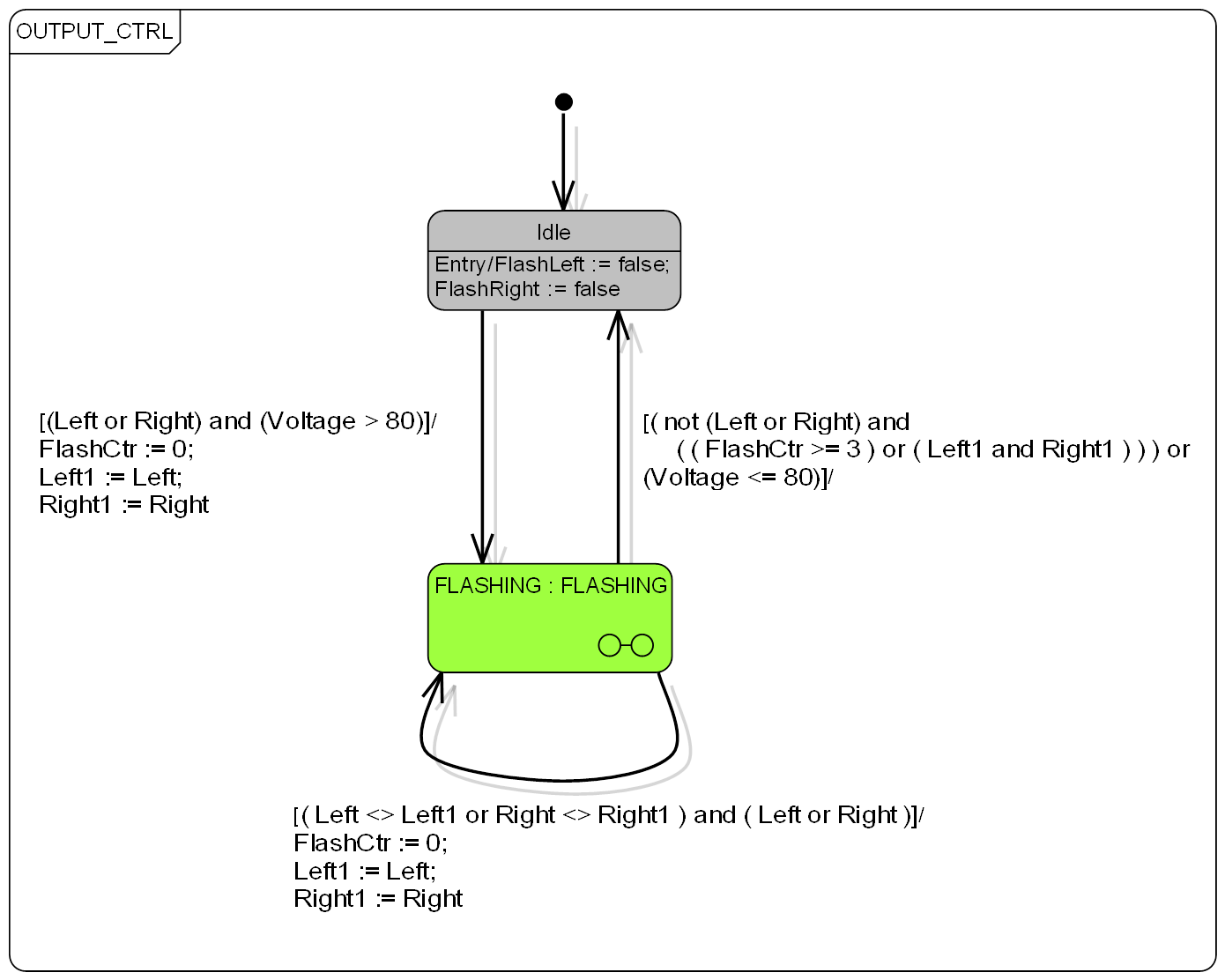
Figure 8: State machine switching indication lights.

Table 2: Requirements and associated constraints identifying witness computations.

Requirement	Constraint
REQ-001 Flashing requires sufficient voltage	«Constraint» $\mathbf{F}(Voltage\leq 80)$
REQ-002 Flashing with 340ms/320ms on-off periods	«Transition» $\text{ON}\rightarrow\text{OFF}$ «Transition» $\text{OFF}\rightarrow\text{ON}$
REQ-003 Switch on turn indication left	«Constraint» $\mathbf{F}(\text{FlashLeft}=1\wedge\text{FlashRight}=0)$
REQ-004 Switch on turn indication right	«Constraint» $\mathbf{F}(\text{FlashLeft}=0\wedge\text{FlashRight}=1)$
REQ-005 Emergency flashing on overrides left/right flashing	«Constraint» $\mathbf{F}(\text{EMER\_OFF}\wedge\text{TurnIndLvr}>0\wedge\text{EmerFlash})$
REQ-006 Left-/right flashing overrides emergency flashing	«Atomic State» TURN_IND_OVERRIDE
REQ-007 Resume emergency flashing	«Transition»$\text{TURN\_IND\_OVERRIDE}\rightarrow\text{EMER\_ACTIVE}$
REQ-008 Resume turn indication flashing	«Constraint» $\mathbf{F}(\text{EMER\_ACTIVE}\wedge\neg\text{EmerFlash}\wedge\text{TurnIndLvr}>0)$
REQ-009 Tip flashing	«Constraint» $\mathbf{F}(\text{Voltage}>80\wedge\neg(\text{Left}\vee\text{Right})\wedge\text{Left1}+\text{Right1}=1\wedge\text{FlashCtr}<3)$

References

- [1]
- [2] AERONAUTICAL RADIO, INC. (2009): Aircraft Data Network, Part 7, Avionics Full-Duplex Switched Ethernet Network. AERONAUTICAL RADIO, INC., 2551 Riva Road, Annapolis, Maryland 21401-7435.
- [3] Paul Baker, Oystein Haugen, Zhen Ru Dai, Clay Williams & Jens Grabowski (2008): Model-Driven Testing – Using the UML Testing Profile. Springer, Berlin Heidelberg.
- [4] Armin Biere, Alessandro Cimatti, Edmund M. Clarke & Yunshan Zhu (1999): Symbolic Model Checking without BDDs. In: Proceedings of the 5th International Conference on Tools and Algorithms for Construction and Analysis of Systems, TACAS ’99, Springer-Verlag, London, UK, UK, pp. 193–207, 10.1007/3-540-49059-0_14.
- [5] Armin Biere, Keijo Heljanko, Tommi Junttila, Timo Latvala & Viktor Schuppan (2006): Linear Encodings of Bounded LTL Model Checking. Logical Methods in Computer Science 2(5), pp. 1–64, 10.2168/LMCS-2(5:5)2006.
- [6] Jörg Brauer, Jan Peleska & Uwe Schulze (2012): Efficient and Trustworthy Tool Qualification for Model-Based Testing Tools. In Brian Nielsen & Carsten Weise, editors: Testing Software and Systems. Proceedings of the 24th IFIP WG 6.1 International Conference, ICTSS 2012, Aalborg, Denmark, November 2012, Lecture Notes in Computer Science 7641, Springer, Heidelberg Dordrecht London New York, pp. 8–23, 10.1007/978-3-642-34691-0_3.
- [7] E. Brinksma (1988): A Theory for the Derivation of Tests. In S. Aggarwal & K. Sabnani, editors: Protocol Specification Testing and Verification VIII (PSTV ‘88), pp. 63–74.
- [8] R. E. Bryant, P. Chauhan, E. M. Clarke & A. Goel (2000): A Theory of Consistency for Modular Synchronous Systems. In W. A. Hunt & S. D. Johnson, editors: Formal Methods in Computer-Aided Design (FMCAD), Lecture Notes in Computer Science 1954, Springer, pp. 486–504, 10.1007/3-540-40922-X_30.
- [9] A. L. C. Calvalcanti & M.-C. Gaudel (2011): Testing for Refinement in Circus. Acta Informatica 48(2), pp. 97–147, 10.1007/s00236-011-0133-z.
- [10] Tsun S. Chow (1978): Testing Software Design Modeled by Finite-State Machines. IEEE Transactions on Software Engineering SE-4(3), pp. 178–186, 10.1109/TSE.1978.231496.
- [11] Edmund M. Clarke, Orna Grumberg & Doron A. Peled (1999): Model Checking. The MIT Press, Cambridge, Massachusetts.
- [12] R. De Nicola & M. Hennessy (1984): Testing Equivalences for Processes. Theoretical Computer Science 34, pp. 83–133, 10.1016/0304-3975(84)90113-0.
- [13] Esterel Technologies: SCADE Suite Product Description. http://www.estereltechnologies.com.
- [14] Wolfgang Grieskamp, Yuri Gurevich, Wolfram Schulte & Margus Veanes (2002): Generating Finite State Machines from Abstract State Machines. ACM SIGSOFT Software Engineering Notes 27(4), pp. 112–122, 10.1145/566171.566190.
- [15] M. Hennessy (1988): Algebraic Theory of Processes. MIT Press, Cambridge, Massachusetts, London.
- [16] C. A. R. Hoare & H. Jifeng (1998): Unifying Theories of Programming. Prentice-Hall.
- [17] Wen ling Huang, Jan Peleska & Uwe Schulze (2013): Test Automation Support. Technical Report D34.1, COMPASS Comprehensive Modelling for Advanced Systems of Systems.
- [18] Wen ling Huang, Jan Peleska & Uwe Schulze (to appear 2014): Specialised Test Strategies. Technical Report D34.2, COMPASS Comprehensive Modelling for Advanced Systems of Systems.
- [19] Wen-ling Huang & Jan Peleska (2012): Specialised Test Strategies. Public Document, COMPASS Comprehensive Modelling for Advanced Systems of Systems.
- [20] (2009): Road Vehicles - Functional Safety - Part 8: Supporting Processes. Technical Report, International Organization for Standardization. ICS 43.040.10.
- [21] ISO/DIS 26262-4 (2009): Road vehicles – functional safety – Part 4: Product development: system level. Technical Report, International Organization for Standardization.
- [22] Helge Loding & Jan Peleska (2010): Timed Moore Automata: Test Data Generation and Model Checking. Software Testing, Verification, and Validation, 2008 International Conference on 0, pp. 449–458, 10.1109/ICST.2010.60.
- [23] Rocco De Nicola & Frits Vaandrager (1990): Action versus State based Logics for Transition Systems. In Irène Guessarian, editor: Semantics of Systems of Concurrent Processe, LNCS 469, Springer-Verlag, Berlin, Heidelberg, pp. 407–419, 10.1007/3-540-53479-2_17.
- [24] Object Management Group (2010): OMG Systems Modeling Language (OMG SysMLTM). Technical Report, Object Management Group. OMG Document Number: formal/2010-06-02.
- [25] OMG (2011): OMG Unified Modeling Language (OMG UML) Superstructure ver. 2.4.1. www.uml.org/spec/UML/2.4.1/Superstructure/PDF/.
- [26] J. Peleska & M. Siegel (1997): Test Automation of Safety-Critical Reactive Systems. South African Computer Jounal 19, pp. 53–77.
- [27] Jan Peleska, Artur Honisch, Florian Lapschies, Helge Löding, Hermann Schmid, Peer Smuda, Elena Vorobev & Cornelia Zahlten (2011): A Real-World Benchmark Model for Testing Concurrent Real-Time Systems in the Automotive Domain. In Burkhart Wolff & Fatiha Zaidi, editors: Testing Software and Systems. Proceedings of the 23rd IFIP WG 6.1 International Conference, ICTSS 2011, LNCS 7019, IFIP WG 6.1, Springer, Heidelberg Dordrecht London New York, pp. 146–161, 10.1007/978-3-642-24580-0_1.
- [28] Jan Peleska, Elena Vorobev & Florian Lapschies (2011): Automated Test Case Generation with SMT-Solving and Abstract Interpretation. In Mihaela Bobaru, Klaus Havelund, Gerard J. Holzmann & Rajeev Joshi, editors: Nasa Formal Methods, Third International Symposium, NFM 2011, LNCS 6617, Springer, Pasadena, CA, USA, pp. 298–312, 10.1007/978-3-642-20398-5_22.
- [29] M. S. Phadke (1989): Quality Engineering Using Robust Design. Prentice Hall, Englewood Cliff, NJ.
- [30] F. Rogin, T. Klotz, G. Fey, R. Drechsler & S. Rulke (2009): Advanced Verification by Automatic Property Generation. IET Computers & Digital Techniques 3(4), pp. 338–353, 10.1049/iet-cdt.2008.0110. Available at http://link.aip.org/link/?CDT/3/338/1.
- [31] A. W. Roscoe (2010): Understanding Concurrent Systems. Springer.
- [32] RTCA SC-205/EUROCAE WG-71 (2011): Model-Based Development and Verification Supplement to DO-178C and DO-278A. RTCA/DO-331, RTCA, Inc., 1140 Connecticut Avenue, N.W., Suite 1020, Washington, D.C. 20036.
- [33] RTCA SC-205/EUROCAE WG-71 (2011): Software Considerations in Airborne Systems and Equipment Certification. RTCA/DO-178C, RTCA, Inc., 1140 Connecticut Avenue, N.W., Suite 1020, Washington, D.C. 20036.
- [34] RTCA,SC-167 (1992): Software Considerations in Airborne Systems and Equipment Certification, RTCA/DO-178B. RTCA.
- [35] S. Schneider (1995): An Operational Semantics for Timed CSP. Information and Computation 116, pp. 193–213, 10.1006/inco.1995.1014.
- [36] S. Schneider (2000): Concurrent and Real-time Systems – The CSP Approach. Wiley and Sons Ltd.
- [37] A. P. Sistla (1994): Liveness and Fairness in Temporal Logic. Formal Aspects of Computing 6(5), pp. 495–512, 10.1007/BF01211865.
- [38] J.G. Springintveld, F.W. Vaandrager & P.R. D’Argenio (2001): Testing timed automata. Theoretical Computer Science 254(1-2), pp. 225–257, 10.1016/S0304-3975(99)00134-6.
- [39] European Committee for Electrotechnical Standardization (2001): EN 50128 – Railway applications – Communications, signalling and processing systems – Software for railway control and protection systems. CENELEC, Brussels.
- [40] Jan Tretmans (1996): Test generation with inputs, outputs and repetitive quiescence. Software – Concepts and Tools 17(3), pp. 103–120.
- [41] Jan Tretmans (1999): Testing Concurrent Systems: A Formal Approach. In J.C.M. Naeten & S. Mauw, editors: CONCUR’99 – Int. Conference on Concurrency Theory, Lecture Notes in Computer Science 1664, Springer, pp. 46–65, 10.1007/3-540-48320-9_6.
- [42] Frits Vaandrager (2012): Active Learning of Extended Finite State Machines. In Brian Nielsen & Carsten Weise, editors: Testing Software and Systems. Proceedings of the 24th IFIP WG 6.1 International Conference, ICTSS 2012, Aalborg, Denmark, November 2012, Lecture Notes in Computer Science 7641, Springer, Heidelberg Dordrecht London New York, pp. 5–7, 10.1007/978-3-642-34691-0_2.
- [43] Stephan Weißleder (2010): Test Models and Coverage Criteria for Automatic Model-Based Test Generation with UML State Machines. Doctoral thesis, Humboldt-University Berlin, Germany.
- [44] J. Woodcock, A. Cavalcanti, J. Fitzgerald, P. Larsen, A. Miyazawa & S. Perry (2012): Features of CML: a Formal Modelling Language for Systems of Systems. IEEE Systems Journal 6, 10.1109/SYSoSE.2012.6384144.