Bistability and chaos at low-level of quanta

Abstract

We study nonlinear phenomena of bistability and chaos at a level of few quanta. For this purpose we consider a single-mode dissipative oscillator with strong Kerr nonlinearity with respect to dissipation rate driven by a monochromatic force as well as by a train of Gaussian pulses. The quantum effects and decoherence in oscillatory mode are investigated on the framework of the purity of states and the Wigner functions calculated from the master equation. We demonstrate the quantum chaotic regime by means of a comparison between the contour plots of the Wigner functions and the strange attractors on the classical Poincaré section. Considering bistability at low-limit of quanta, we analyze what is the minimal level of excitation numbers at which the bistable regime of the system is displayed? We also discuss the formation of oscillatory chaotic regime by varying oscillatory excitation numbers at ranges of few quanta. We demonstrate quantum-interference phenomena that are assisted hysteresis-cycle behavior and quantum chaos for the oscillator driven by the train of Gaussian pulses as well as we establish the border of classical-quantum correspondence for chaotic regimes in the case of strong nonlinearities.

I Introduction

Nonlinear dissipative oscillator (NDO) operated in the quantum regime is becoming significant in both fundamental and applied sciences, particularly, for implementation of basic quantum optical systems, in engineering of nonclassical states and quantum logic. The important implementations have recently been realized in the context of superconducting devices based on the nonlinearity of the Josephson junction (JJ) exhibiting a wide variety of quantum phenomena (see, the Reviews Nori , Nori1 and Mak -Hosk ). In some of these devices, dynamics are analogous to those of a quantum particle in an oscillatory anharmonic potential claud . The single nonlinear oscillator and systems of nonlinear oscillators also consist of basic theoretical models for various nano-electro-mechanical and nano-opto-mechanical devices. In the last decade there was exciting technological advances in the fabrication and control of such devices Craig -ekinci that are attracting interest in a broad variety of research areas and for many possible applications due to their remarkable combination of properties: small mass, high operating frequency, large quality factor, and easily accessible nonlinearity. Nanomechanical oscillators are being developed for a host of nanotechnological applications. They are ideal candidates for probing quantum limits of mechanical motion in an experimental setting. Moreover, they are the basis of various precision measurements Jens -Rug17 , as well as for basic research in the mesoscopic physics of phonons Keith18 , and the general study of the behavior of mechanical degrees of freedom at the interface between the quantum and the classical worlds Miles .

The efficiency of quantum oscillatory effects requires a high nonlinearity with respect to dissipation. However, for weak damping even small nonlinearity can become important. Development of driven NDO in quantum regime requires cooling these systems to their ground state and significant advances have been made in cooling the systems to far below the temperature of the environment Rae -Wang26 .

It is well known that classically, the nonlinearity-induced dependence of the oscillatory frequency or the amplitude usually leads to bistability of the driven NDO drummond . The corresponding systems describe amplifiers which are ubiquitous in experimental physics. The Josephson junction amplifier has been discussed in JBA as a bistable amplifier which has particular interest. The dynamical bifurcation of a rf-biased Josephson junction was proposed to be used as a basis for the amplification of quantum signals in vij1 ; vij2 . Though the bistability has been usually treated as a classical signature of the NDO the quantum dynamics in the bistable region has been a new subject in the past years ep1 -ep4 .

Quantum dynamics of an oscillator is naturally described by Fock states, that have definite numbers of energy quanta. However, these states are hard to create in experiments because excitations of oscillatory systems usually lead to the production of coherent states but not quantum Fock states. Nevertheless, quantum oscillatory states can be prepared and can be manipulated by coupling oscillators to atomic systems driven by classical pulses. The systematic procedure has been proposed in Ref. law and has been demonstrated for deterministic preparation of mechanical oscillatory Fock states with trapped ions mek , in cavity QEDs with Rydberg atoms varc and in solid-state circuit QED for deterministic preparation of photon number states in a resonator by interposing a highly nonlinear Josephson phase qubit between a superconducting resonator hof .

For the NDO in quantum regime the nonlinearity makes frequencies of transitions between adjacent oscillatory energy levels different. Thus, strong nonlinearity enables spectroscopic identification and selective excitation of transitions between Fock states. Thus, it is possible in this regime to prepare the NDO at low-level of quanta. In this approach, it has been shown that the production of Fock states, Fock states superpositions or qubits can also be realized in over-transient regime of an anharmonic dissipative oscillator without any interactions with atomic and spin-1/2 systems and with complete consideration of decoherence effects Gev39 . For this goal the strong Kerr nonlinearity as well as the excitation of resolved lower oscillatory energy levels with a specific train of Gaussian pulses have been considered.

In this paper we consider the NDO in the regime of low-level of excitation for the study of the problems of quantum bistability and chaos. Therefore, the goal of the paper is twofold. In one part, we consider the bistability on a few oscillatory excitation number considering the NDO driven by monochromatic force. The bistability on a few excitation number is attractive for ultra-low power operation, but it has practical problems related with quantum fluctuation-induced spontaneous switching. In this part, we also demonstrate the production of quantum interference between bistable branches for the NDO driven by a train of Gaussian pulses.

The other part of the paper is devoted to investigation of quantum chaos in low-level excitation regime of the pulsed NDO. Much research on the subject of classical and quantum chaos has been done on the base of the kicked rotor, which exhibits regions of regular and chaotic motion. Its experimental realization, and observation of the model’s dissipation and decoherence effects are carried out on a gas of ultracold atoms in a magneto-optical trap subjected to a pulsed standing wave Ammann41 , Klappauf42 . In Ref. Milburn43 it was proposed to realize the parametrically kicked nonlinear oscillator model in a cavity involving Kerr nonlinearity. It was also shown that a more promising realization of this system, including the quantum regime, is achieved in the dynamics of cooled and trapped ions, interacting with a periodic sequence of both standing wave pulses and Gaussian laser pulses Breslin44 . In addition to these and the other important input (see, also Leon , Macc ) in this paper we consider quantum dissipative chaos of the NDO driven by a train of Gaussian pulses in a strong quantum regime and in complete consideration of dissipation and decoherence. In this way, quantum dissipative chaos at the limit of low-level of excitation numbers will be considered.

The paper is arranged as follows. In Sec. II, we shortly describe a pulsed NDO. In Sec. III, we study bistability at a level of few quanta for the NDO driven by monochromatic force. In Sec.IV, we consider the production of quantum interference for bistable regime of the NDO driven by the train of Gaussian pulses. In Sec. V, we study quantum dissipative chaos at limit of low-level of excitation numbers for the NDO driven by the train of Gaussian pulses. We summarize our results in Sec. VI.

II The model: short description

The Hamiltonian of an anharmonic-driven oscillator in the rotating-wave approximation reads as:

$$H=\hbar\Delta a^{\dagger}a+\hbar\chi(a^{\dagger}a)^{2}+\hbar f(t)(\Omega a^{\dagger}+\Omega^{*}a).$$ (1)

Note that time dependent coupling constant $\Omega f(t)$ that is proportional to the amplitude of the driving field consists of Gaussian pulses with duration $T$ which are separated by time intervals $\tau$ as follow

$$f(t)=\sum{e^{-(t-t_{0}-n\tau)^{2}/T^{2}}}.$$ (2)

Here, $a^{\dagger}$, $a$ are the oscillatory creation and annihilation operators, $\chi$ is the nonlinearity strength, and $\Delta=\omega_{0}-\omega$ is the detuning between the mean frequency of the driving field and the frequency of the oscillator. For $f(t)=1$ this Hamiltonian describes nonlinear oscillator driven by a monochromatic force.

The evolution of the system of interest is governed by the following master equation for the reduced density matrix in the interaction picture:

$$\frac{d\rho}{dt}=-\frac{i}{\hbar}[H,\rho]+\sum_{i=1,2}\left(L_{i}\rho L_{i}^{\dagger}-\frac{1}{2}L_{i}^{\dagger}L_{i}\rho-\frac{1}{2}\rho L_{i}^{\dagger}L_{i}\right),$$ (3)

where $L_{1}=\sqrt{(N+1)\gamma}a$ and $L_{2}=\sqrt{N\gamma}a^{\dagger}$ are the Lindblad operators, $\gamma$ is a dissipation rate, and $N$ denotes the mean number of quanta of a heath bath. To study the pure quantum effects we focus below on the cases of very low reservoir temperatures which, however, ought to be still larger than the characteristic temperature $T\gg T_{cr}=\hbar\gamma/k_{B}$.

The Hamiltonian (1) describes wide range of physical systems, including nano-mechanical oscillator, Josephson junction device, optical fibers, quantum dots, quantum scissors. Part of them have been noted in section I. Note, that quantum effects in a NDO with a time-modulated driving force including also pulsed regime have been studied in a series of papers qsch -mpop .

Below, we use numerical simulation of this equation based on quantum state diffusion method (QSD) (see, Ref. qsd and, for example, applications in Refs.qsch -mpop and qsd1 -qsd4 ). For clarity, in our numerical calculation we choose the mean number of reservoir photons $N=0$. Note, that for $N\ll 1$ the above mentioned restriction is valid for the majority of problems of quantum optics and, particularly, for the schemes involving the nano-mechanical oscillator and Josephson junction. In experiments, the nonlinear oscillator based on the current-biased JJ is cooled down to $T=20mK$, which corresponds to $N=0.0013$, whereas, $T_{cr}=10^{-5}$ K, for $\gamma=1MHz$.

In semiclassical approach the corresponding equation of motion for the dimensionless amplitude of oscillatory mode has the following form

$$\frac{d\alpha}{dt}=-i[\Delta+\chi+2|\alpha|^{2}\chi]\alpha+if(t)\Omega-\gamma\alpha.$$ (4)

This equation modifies the standard Duffing equation on the case of the NDO with time-dependent coefficient.

III Bistability at level of a few quanta

At first, we describe the NDO driven by monochromatic force [the case, $f(t)$=1 in the Hamiltonian described by (1)] in bistable regime. In semiclassical approach based on Eq. 4 the bistable dynamics is realized if the following inequalities are satisfied drummond :

$$\chi(\Delta+\chi)<0,~{}~{}~{}~{}~{}~{}~{}~{}~{}~{}~{}~{}~{}~{}~{}~{}~{}$$

$$|(\Delta+\chi)/0.5\gamma|>\sqrt{3},~{}~{}~{}~{}~{}~{}~{}~{}~{}~{}~{}~{}~{}~{}~{}~{}$$

$$\left[1+\frac{27\chi\Omega^{2}}{\left(\Delta+\chi\right)^{3}}+\left(\frac{1.5\gamma}{\Delta+\chi}\right)^{2}\right]^{2}<\left[1-3\left(\frac{\gamma/2}{\chi+\Delta}\right)^{2}\right]^{3}.$$ (5)

In this range of the parameters the typical hysteresis curves depending on detuning $\Delta$ and force amplitude $\Omega$ display the system drummond . This result for the stationary excitation number $n=|\alpha|^{2}$ can be obtained by solving the following equation:

$$|\alpha|^{2}=\frac{\Omega^{2}}{\left(\Delta+\chi+2\chi|\alpha|^{2}\right)^{2}+\left(\gamma/2\right)^{2}}$$ (6)

and is depicted in Fig. 1.

It is well known that whereas the semiclassical result exhibits hysteresis-cycle behavior, the corresponding quantum mechanical result, which accounts for the influence of quantum noise, shows a gradual evolution. It is seen from the exact quantum solution for the mean excitation number in the following form:

$$\langle a^{\dagger}a\rangle=\frac{\Omega^{2}}{(\Delta+\chi)^{2}+(\gamma/2)^{2}}\frac{F(c+1,c^{*}+1,z)}{F(c,c^{*},z)},$$ (7)

where $F=F_{2}$ is the generalized hypergeometric function, $c$ and $z$ are coefficients that depend on the parameters: $c=(\Delta+\chi)/\chi-i\gamma/(2\chi)$ and $z=2(\Omega/\chi)^{2}$.

It is also seen that the characteristic threshold behavior, determined by a drastic increase of the intensity in the transition region, disappears as the relative nonlinearity $\chi/\gamma$ increases. In Fig. 1 we plot both quantum and semiclassical solutions corresponding to Eqs. 6,7.

More detailed information on the quantum statistical properties of the oscillatory mode in the bistable range can be obtained from the analysis of the excitation number probability distribution function $p(n)$. In this way, the locations of extrema of the $p(n)$-function, i.e. the locations of the most and least probable values of $n$, may be identified with the semiclassical stable and unstable steady states in the limit of small quantum noise level a33 . With the increase of $\chi/\gamma$ the curve of locations of these extrema as depending on $\Omega$ becomes shifted from the corresponding semiclassical curve for the mean excitation number.

Figure 1: (Color online) The mean excitation numbers of anharmonic oscillator: (1) quantum solution, (2) semiclassical solution. The parameters are as follows: $\Delta/\gamma=-15$, $\chi/\gamma=2$.

Considering bistability at low-limit of quanta, for strong quantum regime, it is naturally to put the question what is the minimal level of excitation numbers at which bistable regime is displayed? Below, we discuss this problem on the base of quantum trajectories and the Wigner function to discuss quantum dynamics and on the Poincaré section to discuss semiclassical dynamics.

Analyzing the monochromatically driven NDO for strong quantum regime and in over transient time intervals, $t\gg\gamma^{-1}$, we use numerical method but not the analytical results obtained in terms of the exact solution of the Fokker-Planck equation a33 - i34 . The reason is that the steady-state solution of the Fokker-Planck equation has been found using the standard approximation method of potential equations. The validity of this solution has not been checked up to now in the strong quantum regime that requires a high nonlinearity with respect to dissipation.

We use the Wigner function

$$W(r,\theta)=\sum_{n,m}\rho_{nm}(t)W_{mn}(r,\theta)$$ (8)

in terms of the matrix elements $\rho_{nm}=\langle n|\rho|m\rangle$ of the density matrix operator in the Fock state representation. Here $(r,\theta)$ are the polar coordinates in the complex phase space plane, $x=r\cos\theta$, $y=r\sin\theta$, while the coefficients $W_{mn}(r,\theta)$ are the Fourier transform of matrix elements of the Wigner characteristic function.

The properties of bistable dynamics at the level of a few excitation number are demonstrated on Fig. 2. Fig. 2(a) shows that the mean excitation number is small which means that the system is operated in a deep quantum regime. Analyzing one single quantum stochastic trajectory for excitation numbers on Fig. 2(d) we set the system initially to the vacuum oscillatory state and consider time-dependence over a long time, compared to the characteristic dissipative time. As expected, the analysis of the time-dependent stochastic trajectories for an expectation number shows that the system spends most of its time close to one of the semiclassical bistable solutions with quantum interstate transitions, occurring at random intervals.

Figure 2: (Color online) The mean excitation numbers of oscillatory mode (a), the Wigner function (b), semiclassical Poincaré section (c) , the time evolution of the excitation numbers along a single trajectory (d). The parameters are as follows: $\Delta/\gamma=-8$, $\chi/\gamma=2$, and $\Omega/\gamma=2.7$

In order to demonstrate the bistability in phase-space we tune the nonlinear oscillator parameters to satisfy inequalities Eq. (5). As calculations show the Wigner function displays two peaks (Fig. 2(b)) that displays bistability, whereas Poincaré section obtained from the semi-classical calculations of Eq. (4) shows a single point in phase space (Fig.  2(c)) that corresponds to the regular dynamics.

Figure 3: (Color online) The Wigner functions for oscillatory mode in dependence on the amplitude. The parameters are as follows: $\Delta/\gamma=-8$, $\chi/\gamma=2$, and (a) $\Omega/\gamma=2.1$, (b) $\Omega/\gamma=2.3$, (c) $\Omega/\gamma=2.5$, (d) $\Omega/\gamma=2.7$, (e) $\Omega/\gamma=2.9$, (f) $\Omega/\gamma=3.1$.

Further investigation of this model allows to establish other properties of dissipative bistable dynamics. For this goal on the Fig. 3 we show bistability in phase-space depending on the amplitude of the external force. As we see for the given parameters of detuning and nonlinearity there is an intermediate range of amplitudes where bistability takes place.

It is also interesting to consider behavior of the NDO by using the scaling properties of Eq. (4). Indeed, it is easy to verify that this equation is invariant with respect to the following scaling transformation of the complex amplitude: $\alpha^{{}^{\prime}}\rightarrow\lambda\alpha,\chi^{{}^{\prime}}\rightarrow\chi/\lambda^{2},\Omega^{{}^{\prime}}\rightarrow\lambda\Omega,\Delta^{{}^{\prime}}\rightarrow\Delta+\chi(1-1/\lambda^{2})$. Thus, for $\lambda>1$ oscillatory excitation numbers are increased during scaling transformation. It is interesting to analyze such scaling from the point of view of quantum-statistical theory and its relevance for decoherence and dissipation. Thus, using the scaling properties we consider the system for various excitation numbers. The Wigner functions for the scaled $\lambda=2$ and $\lambda=3$ are presented in Fig. 4. As we see, increasing $\lambda$ leads to the suppression of one of the peaks in the Wigner function and on the whole the bistability of the system is vanished. Thus, we show that such parameter scaling does not occur for strong quantum regime of NDO.

Figure 4: (Color online) (a) The Wigner function for $\lambda=2$, (b) the Wigner function for $\lambda=3$. The parameters are as follows: $\Delta/\gamma=-8$, $\chi/\gamma=2$, and $\Omega/\gamma=2.7$

There is a boundary to detect bistable states at limit of small excitation numbers in phase-space in accordance with Planck uncertainty principle. Taking into account that $\Delta X\Delta P\geq 1/2$, where $X$ and $P$ are dimensionless position and momentum operators and $n=|\alpha|^{2}$, $\alpha=X+iP$, it seems that for small enough level of excitation numbers we cannot distinguish two branches of bistability. In this case sizes of contour plots of Wigner functions are sufficiently squeezed such that two bistable branches are too close to each other to be distinguishable.

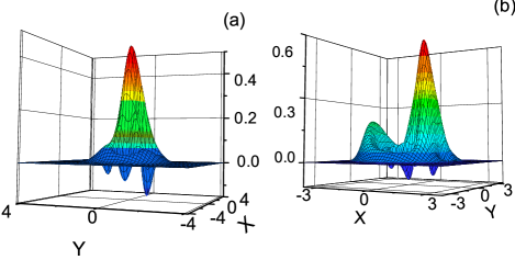
Figure 5: (Color online) The Wigner functions showing quantum interference fringes. The parameters are as follows: $\Delta/\gamma=-8$, $\chi/\gamma=2$, $\Omega/\gamma=2.7$, (a) $T=0.5\gamma^{-1}$ $\tau=2\gamma^{-1}$, (b) $T=0.1\gamma^{-1}$, and $\tau=2\gamma^{-1}$

.

Figure 6: The purity depending from $T$ for fixed $\tau=2.5\gamma^{-1}$ (a), the purity depending from $\tau$ for fixed $T=0.5\gamma^{-1}$ (b). The other parameters are: $\Delta/\gamma=-8$, $\chi/\gamma=2$, and $\Omega/\gamma=2.7$.

IV Quantum interference assisted by bistability

In this section we demonstrate that it is possible to create quantum superposition in bistable dynamics of the NDO under pulsed excitation. Really, the application of time-dependent force can lead to transition between two branches of the system dynamics in the bistable regime and open an opportunity to generate interference between them. However, quantum interference takes place for very short time intervals and disappears due to dissipation and decoherence. In order to recover the quantum interference for over transient regimes we suggest to apply the specific train of Gaussian pulses according to the model considered in section II. The results depicted on Fig. 5 shows that with applied Gaussian pulse the Wigner function has negative ranges. The Wigner functions describe two humps corresponding to bistable branches and interference pattern between them in phase-space.

In order to be sure that effects of dissipation and decoherence in oscillatory mode for transient time are suppressed if the train of pulses is applied we calculate the purity of the state, i.e. $Tr(\rho^{2})$. For a pure state $Tr(\rho^{2})=1$. The results for $Tr(\rho^{2})$ are depicted in Fig. 6 for over-transient regime, i.e. for time intervals, $t\gg\gamma^{-1}$, in dependence on the pulse duration $T$ and time-intervals between pulses $\tau$. The Fig. 6(a) corresponds to the case of fixed $\tau$ , i.e. $\tau=2.5$. Considering the dependence from the duration of pulses for this case we conclude that the purity is maximal for very short pulses and lost with increasing of $T$. The opposite behavior for the fixed interval between pulses is realized in Fig. 6(b).

V Quantum dissipative chaos at low-level of excitation numbers

In this section we demonstrate that dissipative chaos is realized in strong quantum regime NDO on low-level of oscillatory excitation numbers. Chaotic regime appears in the NDO driven by train of Gaussian pulses, and it depends on the duration $T$ of the pulses and the time intervals $\tau$ between them.

Many criteria have been suggested to define chaos in quantum systems, varying in their emphasis and domain of application. Nevertheless, as yet, there is no universally accepted definition of quantum chaos. Our analysis is given in the framework of semiclassical and quantum distributions by using a correspondence between contour plots of the Wigner function and the Poincaré section. Such analysis has been proposed and realized AMK1 in mesoscopic regimes of NDO with time-dependent coefficients.

It is well known that the Poincaré section has the form of strange attractor in phase space for dissipative chaotic systems while it has the form of close contours with separatrices for Hamiltonian systems. Thus, in this paper we demonstrate the quantum chaotic regime by means of a comparison between the contour plots of the Wigner functions and the strange attractors on the classical Poincaré section. In this way, we calculate the Wigner function in phase space by averaging an ensemble of quantum trajectories for definite time intervals. On the other hand, the Poincaré section is calculated through the semiclassical distribution based on Eq. 4 but for a large number of time intervals: it is constructed by fixing points in phase space at a sequence of periodic intervals. Note, that such analysis seems to be rather qualitative than quantitative for strong quantum regime and the ranges of low-level oscillatory excitation numbers, where the validity of semiclassical equation is questionable. Indeed, it is shown below that semiclassical and quantum treatment of quantum dissipative chaos are cardinally different in the deep quantum regime.

The typical results of calculations are depicted below. Note, that the ensemble-averaged mean oscillatory excitation number and the Wigner functions are nonstationary and exhibit a periodic time dependent behavior, i.e. they repeat the periodicity of the driving pulses at the over transient regime. In this nonstationary regime the Poincaré section depends on the initial time-interval $t_{0}$. We choose various initial time $t_{0}$ in order to ensure that they match to the corresponding time-intervals of the Wigner function. In Figs. 7, 8, 9 and 10, we show the typical semiclassical and quantum distributions for the parameters $\Delta/\gamma$, $\chi/\gamma$, $\Omega/\gamma$ corresponding to the chaotic regimes and for various durations of the Gaussian pulses.

Figure 7: (Color online)(a)The Poincaré section, (b)the contour plot of the Wigner function, (c)the excitation number time series with snapshots of Gaussian pulses as inset, and (d) the Wigner function. The parameters are as follows: $\chi/\gamma=0.7$, $\Omega/\gamma=20.4$, $\Delta/\gamma=-15$, $T=0.25\gamma^{-1}$, $\tau=2\pi/5\gamma$. Note that these distributions occur at time $\gamma t=100$ with the mean excitation number of $1.54$. The range of excitation numbers are $1.26$ to $4.98$.

Figure 8: (Color online)(a) The Poincaré section, (b) the contour plot of Wigner function, (c) the excitation number time series with snapshots of Gaussian pulses as inset, and (d)the Wigner function. The parameters are: $\chi/\gamma=0.7$, $\Omega/\gamma=20.4$, $\Delta/\gamma=-15$, $T=0.205\gamma^{-1}$, $\tau=2\pi/5\gamma$. Note that these distributions occur at time $\gamma t=100$ with the mean excitation number of $1.74$. The range of excitation numbers are $1.29$ to $5.11$.

Figure 9: (Color online)(a) The Poincaré section, (b) the contour plot of Wigner function, (c) the excitation number time series with snapshots of Gaussian pulses as inset, and (d) the Wigner function. The parameters are: $\chi/\gamma=0.7$, $\Omega/\gamma=20.4$, $\Delta/\gamma=-15$, $T=0.15\gamma^{-1}$, $\tau=2\pi/5\gamma$. Note that these distributions occur at time $\gamma t=100$ with the mean excitation number of $2.04$. The range of excitation numbers are $1.43$ to $5.13$.

Figure 10: (Color online)(a) The Poincaré section, (b) the contour plot of Wigner function, (c) the excitation number time series with snapshots of Gaussian pulses as inset, and (d) the Wigner function. The parameters are: $\chi/\gamma=0.7$, $\Omega/\gamma=20.4$, $\Delta/\gamma=-15$, $T=0.1\gamma^{-1}$, $\tau=2\pi/5\gamma$. Note that these distributions occur at time $\gamma t=100$ with the mean excitation number of $2.46$. The range of excitation numbers are $1.62$ to $4.83$.

As we see, the figures of Poincaré sections clearly indicate a classical strange attractor with fractal structure that is typical of chaotic dynamics. The Wigner functions have spiral (helical) structures (Figs. 7 to 10) that reflect chaotic regime in analogy with the corresponding Poincaré sections, and their contour plots are concentrated approximately around the attractor. Nevertheless, in this deep quantum regime the different branches of the attractors are hardly resolved in the Wigner functions.

It should be specified that the Wigner function for the regime presented in Fig. 10 has region of negative values. Obviously, this fact reflects on quantum effects in the chaotic regime.

The chaotic dynamics of the oscillatory mode strongly depends on the time-interval $t$. To demonstrate this point in Figs. 11 and 12, we depict the Wigner function and the Poincaré section for the oscillatory parameters used in Fig. 10, however, for the other time-intervals of $t$ within the duration of pulses which correspond to the maximal and minimal values of the number of excitation number.

Figure 11: (Color online)(a) The Poincaré section, (b) the excitation number time series, (c) the contour plot of Wigner function, and (d) the Wigner’s function at the moment $\gamma t=100.6$ when the excitation number is maximum. The parameters are: $\chi/\gamma=0.7$, $\Omega/\gamma=20.4$, $\Delta/\gamma=-15$, $T=0.1\gamma^{-1}$, $\tau=2\pi/5\gamma$.

Figure 12: (Color online)(a) The Poincaré section, (b) the excitation number time series, (c) the contour plot of Wigner function, and (d) the Wigner’s function at the moment $\gamma t=100.4$ when the excitation number is minimum. The parameters are as follows: $\chi/\gamma=0.7$, $\Omega/\gamma=20.4$, $\Delta/\gamma=-15$, $T=0.1\gamma^{-1}$, $\tau=2\pi/5\gamma$.

In the end of this section, we explore the transition from regular to chaotic regimes that are realized through varying the strength of the pulse trains by considering cases of small excitation number. For this goal, we present at first the results in semiclassical approximation based on an analysis of the Lyapunov exponents of the semi-classical time series sprott . This quantity is determined as $L=\frac{1}{\Delta t}\ln\frac{\|x_{2}(t)-x_{1}(t)\|}{\|x_{2}(t_{0})-x_{1}(t_{0})\|}$, here $x=\left(Re(\alpha),Im(\alpha),\beta\right)$, where $\beta$ is the time variable defined through $d\beta/dt=1$ which augments Eq. (4) to create an autonomous system. Note that $x_{2}$ and $x_{1}$ represent two trajectories that are very close together at the initial time $t_{0}$. Furthermore, $\Delta t=t-t_{0}$, with $t\rightarrow\infty$. For $L>0$ the system shows chaotic dynamics. $L=0$ corresponds to the case of conservative regular systems, and $L<0$ indicates that the dissipative system is regular. We examine the exponents for time intervals corresponding to the minimal and maximal excitation numbers of the oscillatory mode in dependence from the parameter $\Omega/\gamma$. The results are depicted in Figs. 13 and 14 for the constant parameters: $\Delta/\gamma$ and $\chi/\gamma$. We observe a transition from regular to chaotic behavior at $\Omega/\gamma=12.55$ for minimal and maximal excitation number of the oscillatory mode. Note that this transition occurs at the strong quantum regime as the excitation number ranges from the minimum $n=0.94$ to the maximum $n=2.70$. Thus, when the strength of the pulse trains $\Omega/\gamma$ is low, we observe regular behaviour; and as a critical threshold is crossed, the system behaves chaotically. Interestingly, a closer scrutiny of the dynamics of the system reveals a regime of transient chaos in the range $17.61\leq\Omega/\gamma\leq 19.56$, whereupon the semi-classical dynamics rattle about chaotically for some time before settling down to regular behaviour which leads to a window of negative Lyapunov exponents. Then, beyond $\Omega/\gamma=19.56$, chaotic attractors are found to emerge again in the Poincaré section. It is important to note that analogous dynamical behavior are observed to arise at both the moments when the excitation number is a minimum and a maximum (see Fig. 13).

Figure 13: (Color online) The largest Lyapunov exponent of the semi-classical dynamics versus the strength of the pulse trains. The solid (blue) curve corresponds to the moment of maximum excitation number at $\gamma t=39.1$ for $1\leq\Omega/\gamma\leq 19$ and at $\gamma t=39$ for $19.5\leq\Omega/\gamma\leq 26$. The dashed (red) curve corresponds to the moment of minimum excitation number at $\gamma t=40.2$ for $1\leq\Omega/\gamma\leq 8.5$ and at $\gamma t=40.1$ for $9\leq\Omega/\gamma\leq 26$. The rest of the parameters are: $\chi/\gamma=0.7$, $\Delta/\gamma=-15$, $T=0.1\gamma^{-1}$, $\tau=2\pi/5\gamma$.

Figure 14: (Color online) The plot of the maximum and minimum excitation number versus the strength of the pulse trains that correspond to the case of Fig. 13. The solid (blue) curve is for the maximum excitation number and the dashed (red) curve for the minimum excitation number. Note that the regular, transient chaos, and chaos regimes of the corresponding semi-classical dynamics are also indicated in the plot.

In summary, we have uncovered the parameters for which decreasing of the excitation number leads to a transition of the system from chaotic to regular regime in the classical treatment. Another situation is realized in the quantum treatment. Indeed, for these regimes of low-excitation, quantum noise and quantum effects play essential role in forming of the oscillatory dynamics, particularly, in realization of chaotic dynamics and scenarios of transition from chaotic to regular regime. This statement is also confirmed by the calculation of the Wigner function. We observe that below the transition threshold of $\Omega/\gamma=12.55$, the Wigner function has the form of a single hump. Beyond the transition threshold, the hump starts to spread and spiral begins to form. These changes are found to happen continuously and smoothly in the Wigner function as $\Omega/\gamma$ increases. However, as $\Omega/\gamma$ goes above $19.56$, the Wigner functions are observed to quickly take the appearance of a strange attractor. Our results here thus clearly show the presence of good quantum-classical correspondence in the quantum and classical dynamical behaviour. In addition, our results also demonstrate that a quantum NDO, which is a form of quantum anharmonic oscillators, possess a rich set of dynamical behaviour and properties that may be potentially useful for many practical purposes cnn_pre ; cnn_pra .

VI Summary

To summarize, we have studied the problem of quantum chaos and bistability at level of few excitation numbers of NDO that is interacting with an external field and a background environment leading to dissipation and decoherence. We have analyzed the formation of bistable behavior and chaotic regime of NDO in strong quantum regime when the ratio $\chi/\gamma$ is chose from $0.7$ to $2$ . We use a systematic numerical analysis based on numerical simulation of master equation by using quantum state diffusion method of quantum trajectories where we have varied a number of relevant oscillatory parameters: $\Omega/\gamma$, $\Delta/\gamma$ as well as the parameters of Gaussian pulses. Thus, the combination of the results provides a rather thorough understanding of the NDO in strong quantum regime as well as have presented a simple picture to understand the formation of bistability and chaos at low-level of quanta in phase-space. We have also found unexpected features of NDO in phase-space. It has been demonstrated that the Wigner functions of oscillatory mode in both bistable and chaotic regimes realized due to interaction with train of Gaussian pulses acquire negative values and interference patterns in parts of phase-space. We have demonstrated that in the case of bistable dynamics the Wigner functions describe two humps corresponding to bistable branches and interference pattern between them in phase-space while for the chaotic regime the Wigner functions have spiral structures, (which correspond to strange attractor in Poincaré sections), with deep well showing negativity of the Wigner function (Fig. 10 (d)). Quantum interference in phase-space is realized in over transient regime due to driving the oscillator by series of short pulses with proper parameters for effective reducing of dissipative and decoherence effects. Our results can be tested with available experimental systems noted in the section I.

References

- (1) J. Q. You and F. Nori, Nature 474, 585 (2011).
- (2) Iulia Buluta, Sahel Ashhab and Franco Nori, Rep. Prog. Phys. 74, 104401 (2011).
- (3) Y. Makhlin, G. Schön, A. Shnirman, Rev. Mod. Phys. 73, 357 (2001).
- (4) D. I. Schuster, et al., Nature 445, 515 (2007).
- (5) A. Fragner, et al., Science 322, 1357 (2008).
- (6) O. Astafiev, et al., Nature 449, 588 (2007).
- (7) M. Neeley, et al., Science 325, 722 (2009).
- (8) O. Astafiev, et al., Science 327, 840 (2010).
- (9) E. Hoskinson, et al., Phys. Rev. Lett. 102, 097004 (2009).
- (10) J. Claudon, A. Zazunov, F. W. J. Hekking, O. Buisson, Phys. Rev. B 78, 184503 (2008).
- (11) H. G. Craighead, Science, 290, 1532 (2000).
- (12) M. L. Roukes, Physics World, 14, 25 (2001).
- (13) A. N. Cleland. Foundations of Nanomechanics. Springer, Berlin, 2003.
- (14) K. L. Ekinci and M. L. Roukes, Review of Scientific Instruments, 76, 061101 (2005).
- (15) Jensen, K., Kwanpyo, K. and Zettl. A, Nature Nanotech. 3, 533 (2008).
- (16) Cleland, A. and Roukes, M., Nature 392, 160 (1998).
- (17) Rugar, D., Budakian, R., Mamin, H. and Chui, B. Nature 430, 329 (2004).
- (18) Keith C. Schwab, E. A. Henriksen, J. M. Worlock, and Michael L. Roukes, Nature 404, 974 (2000).
- (19) Miles P. Blencowe. Physics Reports, 395, 159 (2004).
- (20) I. Wilson-Rae, N. Nooshi, W. Zwerger and T. J. Kippenberg Phys. Rev. Lett. 99, 093901 (2007).
- (21) F. Marquardt, J. P. Chen, A. A. Clerk and S. M. Girvin Phys. Rev. Lett. 99, 093902 (2007)
- (22) T. Rocheleau, T. Ndukum, C. Macklin, J. B. Hertzberg, A. A. Clerk and K. C. Schwab, Nature 463, 72 (2010).
- (23) A. D. O’Connell, et al Nature 464, 697 (2010).
- (24) J. D. Teufel, T. Donner, Li Dale, J. H. Harlow, M. S. Allman, K. Cicak, A. J. Sirois, J. D. Whittaker, K. W. Lehnert and R. W. Simmonds, Nature 475, 35 (2011).
- (25) J. Chan, T. P. Mayer Alegre, A. H. Safavi-Naeini, J. T. Hill, A. Krause, S. Gröblacher, M. Aspelmeyer and O. Painter, Nature 478, 89 2011.
- (26) Xiaoting Wang, S. Vinjanampathy, F. W. Strauch, and K. Jacobs, Phys. Rev. Lett. 107, 177204 (2011).
- (27) Drummond P. D. and Walls D. F.,J. Phys. A: Math. Gen. 13, 725, (1980).
- (28) Vijay R., Devoret M. H., and Siddiqi I., Rev. of Scientific Instruments, 80, 111101, 2009.
- (29) I. Siddiqi, R. Vijay, F. Pierre, C. M. Wilson, M. Metcalfe, C. Rigetti, L. Frunzio, and M. H. Devoret, Phys. Rev. Lett., 93, 207002, (2004).
- (30) I. Siddiqi, R. Vijay, F. Pierre, C. M. Wilson, L. Frunzio, M. Metcalfe, C. Rigetti, R. J. Schoelkopf, M. H. Devoret, D. Vion, D. Esteve, Phys. Rev. Lett., 94, 027005, (2005)
- (31) I. Katz, A. Retzker, R. Straub, and R. Lifshitz, Phys. Rev. Lett. 99, 040404, (2007).
- (32) V. Peano and M. Thorwart, Chem. Phys., 322, 135, (2006).
- (33) M. Marthaler and M. I. Dykman, Phys. Rev. A, 73, 042108, (2006).
- (34) M. I. Dykman, Phys. Rev. E, 75, 011101, (2007).
- (35) C. K. Law, J. H. Eberly, Phys. Rev. Lett. 76, 1055 (1996).
- (36) D. M. Meekhof, C. Monroe, B. E. King, W. M. Itano, D. J. Wineland, Phys. Rev. Lett. 76, 1796 (1996).
- (37) B. T. H. Varcoe, et al., Nature 403, 743 (2000); P. Bertet, et al., Phys. Rev. Lett. 88, 143601 (2002); E. Waks, E. Dimanti, Y. Yamamoto, N. J. Phys. 8, 4 (2006).
- (38) M. Hofheinz, et al., Nature 454, 310 (2008); Nature 459, 546 (2009).
- (39) T. V. Gevorgyan, A. R. Shahinyan, G. Yu. Kryuchkyan, Phys.Rev. A 85, 053802 (2012).
- (40) H. Ammann, R. Gray, I. Shvarchuck, and N. Christensen, Phys. Rev. Lett. 80, 4111 (1998).
- (41) B. G. Klappauf, W. H. Oskay, D. A. Steck, and M. G. Raizen, Phys. Rev. Lett. 81, 1203 (1998); 82, 241 (1999).
- (42) G. J. Milburn and C. A. Holmes, Phys. Rev. A 44, 4704 (1991).
- (43) J. K. Breslin, C. A. Holmes, and G. J. Milburn, Phys. Rev. A 56, 3022 (1997); A. J. Scott, C.A. Holmes, and G. J. Milburn, ibid. 61, 013401 (1999).
- (44) W. Léonski, A. Kowalewska-Kudleszuk, Progress in Optics 56, 131 (2011); A. Miranowicz, W. Léonski, J. Opt. B: Quantum Semiclass. Opt. 6, 943 (2004).
- (45) M. A. Macovei, Phys. Rev. A 82, 063815 (2010).
- (46) T. V. Gevorgyan, A. R. Shahinyan, and G. Yu. Kryuchkyan, Phys. Rev. A, 79, 053828, (2009).
- (47) H. H. Adamyan, S. B. Manvelyan and G. Yu. Kryuchkyan, Phys. Rev. A, 63, 022102, (2001).
- (48) H. H. Adamyan, S. B. Manvelyan and G. Yu. Kryuchkyan, Phys. Rev. E, 64, 046219, (2001).
- (49) G. Yu. Kryuchkyan and S. B. Manvelyan, Phys. Rev. Lett., 88, 094101, (2002).
- (50) G. Yu. Kryuchkyan and S. B. Manvelyan, Phys. Rev. A, 68, 013823, (2003).
- (51) T. V. Gevorgyan, S. B. Manvelyan, A. R. Shahinyan, G. Yu. Kryuchkyan, Dissipative Chaos in Quantum Distributions. In: Modern Optics and Photonics: Atoms and Structured Media. Eds: G. Kryuchkyan, G. Gurzadyan and A. Papoyan, World Scientific, 2010.
- (52) I. C. Percival, Quantum State Diffusion, Cambridge University Press, Cambridge, (2000).
- (53) S. T. Gevorkyan, G. Yu. Kryuchkyan and N. T. Muradyan, Phys. Rev. A, 61, 043805 (2000).
- (54) G. Yu. Kryuchkyan and N. T. Muradyan, Phys. Lett. A, 286, 113 (2001).
- (55) H. H. Adamyan and G. Yu. Kryuchkyan, Phys. Rev. A, 74, 023810 (2006).
- (56) N. H. Adamyan, H. H. Adamyan and G. Yu. Kryuchkyan, Phys. Rev.A, 77, 023820 (2008).
- (57) G. Yu. Kryuchkyan and K. V. Kheruntsyan, Opt. Comm., 120, 132, (1996).
- (58) K. V. Kheruntsyan, et al., Opt. Comm. 139, 157, (1997).
- (59) K. V. Kherunstyan, J. Opt. B: Quantum Simclassical Opt., 1,225, (1999).
- (60) J. C. Sprott, Chaos and Time-Series Analysis, Oxford University Press, Oxford, (2003).
- (61) N. N. Chung and L. Y. Chew, Phys. Rev. E, 80, 016204, (2009).
- (62) N. N. Chung and L. Y. Chew, Phys. Rev. A, 80, 012103, (2009).