Diffuse Galactic Light in the Field of the Translucent High Galactic Latitude Cloud MBM32

Abstract

We have conducted B, g, V, and R-band imaging in a $45\arcmin\times 40\arcmin$ field containing part of the high Galactic latitude translucent cloud MBM32, and correlated the intensity of diffuse optical light $S_{\nu}(\lambda)$ with that of 100$\micron$ emission $S_{\nu}(100\micron)$. A $\chi^{2}$ minimum analysis is applied to fit a linear function to the measured correlation and derive the slope parameter $b(\lambda)=\Delta S_{\nu}({\lambda})/\Delta S_{\nu}(100\micron)$ of the best-fit linear function. Compiling a sample by combining our $b(\lambda)$ and published ones, we show that the $b(\lambda)$ strength varies from cloud to cloud by a factor of 4. Finding that $b(\lambda)$ decreases as $S_{\nu}(100\micron)$ increases in the sample, we suggest that a non-linear correlation including a quadratic term of $S_{\nu}(100\micron)^{2}$ should be fitted to the measured correlation. The variation of optical depth, which is $A_{V}$ = 0.16 - 2.0 in the sample, can change $b(\lambda)$ by a factor of 2 - 3. There would be some contribution to the large $b(\lambda)$ variation from the forward-scattering characteristic of dust grains which is coupled to the non-isotropic interstellar radiation field (ISRF). Models of the scattering of diffuse Galactic light (DGL) underestimate the $b(\lambda)$ values by a factor of 2. This could be reconciled by deficiency in UV photons in the ISRF or by a moderate increase in dust albedo. Our $b(\lambda)$ spectrum favors a contribution from extended red emission (ERE) to the diffuse optical light; $b(\lambda)$ rises from $B$ to $V$ faster than the models, seems to peak around 6000 Å  and decreases towards long wavelengths. Such a characteristic is expected from the models in which the DGL is combined with ERE.

1 Introduction

A diffuse optical component to the Galactic interstellar medium (ISM), which is called diffuse Galactic light (DGL) or sometimes “optical cirrus,” was noticed in late 1930’s. Extensive studies (e.g., Elvey & Roach 1937; Henyey & Greenstein 1941; van de Hulst & de Jong 1969; Mattila 1979) revealed that the DGL is starlight scattered off by dust grains in the diffuse ISM which is illuminated by the interstellar radiation field (ISRF). The spectrum of the DGL extends to ultraviolet (UV) wavelengths where Witt et al. (1997) made extensive studies of the dust scattering properties. The DGL distribution is strongly concentrated toward the Galactic plane. This concentration is attributed to the forward-scattering characteristic of interstellar dust grains coupled with a non-isotropic distribution of stars.

Over 50 years later, diffuse far-infrared (IR) emission, so-called “IR cirrus,” was discovered in the IR Astronomical Satellite (IRAS) mission (Low et al., 1984). It was quickly shown that the IR cirrus is also visible on photographic material (de Vries & Le Poole 1985; Paley et al. 1991), and suggested that the 100µm brightness varies linearly with extinction in a range of up to $\sim$ 20 MJy sr^-1 (de Vries & Le Poole 1985; Laureijs et al. 1987). Finding good agreement between the structures seen on the optical images and the distribution of the CO emission, Stark (1995) pointed out that the optical images can be used to distinguish variations in the dust column density from those in the molecular column density. These studies indicate that the IR cirrus is the far-IR counterpart of the DGL; far-IR emission in IR cirrus is thermal emission which follows the dust absorption of starlight. It is thus natural to expect a linear correlation between the DGL and far-IR brightness in the optically thin limit. A combination of optical and far-IR observations would give a powerful tool for investigating the dust properties as well as the ISRF in diffuse ISM (e.g., Beichman 1987 and references therein; Guhathakurta & Tyson 1989).

Since the late 1990s, remarkable progress has been made in the optical and far-IR. In the optical, new wide-field CCD cameras make it possible to cover one or more square degrees at a time, providing the uniform sensitivity over a large area and reducing the systematic uncertainty by temporal airglow variations. In the far-IR, Schlegel et al. (1998), hereafter SFD98, published the $IRAS/$DIRBE maps, which are reprocessed all-sky maps, by combining $IRAS$ and DIRBE (Diffuse Infrared Background Experiment on board the Cosmic Background Explorer satellite) data. The $IRAS/$DIRBE maps have DIRBE quality calibration and $IRAS$ resolution and feature removal of point sources as well as of artifacts from the $IRAS$ scan pattern. Recent studies of diffuse optical light benefit from the progress using a wide-field CCD camera and/or the $IRAS/$DIRBE maps. Analysis of diffuse optical light recorded in the $Pioneer$ mission against the $IRAS/$DIRBE 100$\micron$ maps finally led Matsuoka et al. (2011) to report the detection of the cosmic optical background (COB). The DGL is an important foreground to be subtracted from data taken to measure the COB. Thus, studying the DGL distribution is indispensable to a better understanding of the COB.

The present paper mainly focuses on the following issues. The first issue is related to variations in slope parameters, i.e., $\Delta S_{\nu}(\lambda)/\Delta S_{\nu}$(100$\micron$), which is determined by fitting a linear function to the measured intensity of diffuse optical light $S_{\nu}(\lambda)$ as a function of 100$\micron$ intensity $S_{\nu}$(100$\micron$). It has been indicated that slope parameters vary from cloud to cloud by a factor of 3 - 4. For example, Guhathakurta & Tyson (1989) reported the slope parameters scatter by a factor of 3 in their sample of 4 high Galactic latitude clouds, and the slope in a cloud studied by Paley et al. (1991) is 4 times greater than that obtained from blank-sky spectra sampled in 92,000 directions at high latitude (mostly $|b|>$ 30${}^{\circ})$ by Brandt & Draine (2012). What does cause such large variations? Another issue is related to extended red emission (ERE) in the diffuse optical light. ERE detected in the reflection nebula NGC2327 has a broad emission feature with FWHM of 1500Å peaking at 7200Å (Witt & Schild 1988; Gordon et al. 1998). Carrying out a spectroscopic survey of high-latitude cirrus clouds, Szomoru & Guhathakurta (1998) found that the cirrus spectrum does not agree with that of synthetic scattered E-type galaxy spectra, and explained this mismatch by the presence of ERE. Their cirrus ERE feature peaked at 6000Å  and is shifted toward short (bluer) wavelength as compared with ERE in HII regions (peak $\sim$ 8000Å and reflection and planetary nebulae (peak $\sim$ 7000Å). On the other hand, Brandt & Draine (2012) concluded that their blank-sky spectrum is consistent with those expected for their scattering DGL models, finding no evidence of ERE in the diffuse optical light. For broadband observations, some authors favor the presence of ERE in the diffuse optical light (e.g., Gordon et al. 1998; Witt et al. 2008; Matsuoka et al. 2011), while the others suggest the absence of ERE (Zagury et al. 1999; Zagury 2006).

In the course of our program to constrain the COB, we have carried out broadband imaging of a 45′ $\times$ 40′ field which contains a translucent molecular cloud at high Galactic latitude. In section 2, we describe the observations and the data processing details, such as flux calibration, masking, and aperture correction. Correlation analysis of the intensity of diffuse optical light against the 100$\micron$ emission is presented in section 3. In section 4, we use our measurements along with similar measurements in the literature to discuss issues affecting the correlation, and consider implications for dust scattering DGL models. A summary appears in section 5.

2 Observations and Reduction

2.1 Observations

The target field was selected to have the following properties: (1) it is optically thin or translucent at optical wavelengths, and is characterized by a sufficient contrast at 100$\micron$ to be distinguished from the 100$\micron$ background; (2) it is not crowded with stars and does not include bright stars. The first criterion is needed in order to see clearly the correlation between optical 100$\micron$ emission. The second is needed in order to minimize the contamination from stars, especially from the extended halos of bright stars. Using these criteria, we have selected the southern part of MBM32, covering $\sim 1\arcdeg\times 1\fdg 5$. This is a diffuse, translucent molecular cloud with extinction of $A_{V}=0.3-0.5$ (Magnani & de Vries, 1986), and located at a distance of 120 pc (Magnani et al., 1996) at $l$=147$\fdg$2, $b$=40$\fdg$7. The surrounding sky is not a pure blank-sky; thermal far-IR emission from interstellar dust was detected. Based on the $IRAS$/DIRBE 100$\micron$ map, Witt et al. (2008) estimated $A_{V}=0.6$ for the cloud and $A_{V}=0.25$ for the surrounding sky. The 100$\micron$ intensity in the field ranges from 1.4 to 7.0 MJy sr^-1.

Observations were made at Kiso observatory on dark nights in 2011 February, April, and 2012 February. The Sun and the Moon were more than 35 degrees below the horizon when the data were acquired. The optical data were acquired using the 105cm Schmidt telescope with the 2KCCD camera which has 2048 $\times$ 2048 pixels (Itoh et al., 2001). The field of view of the camera is 50′ $\times$ 50′ with a pixel scale of 1$\farcs$5 pixel^-1. The average seeing was $\sim$ 3$\farcs$3. The area of high-quality is approximately 45′ $\times$ 40′, smaller than the field of view of the camera due to using dithering.

In Figure 1, the observed 45′ $\times$ 40′ field is indicated with a white square superimposed on the $IRAS$/DIRBE 100$\micron$ map. Images were obtained at four photometric bands, B, g, V, and R. In order to reduce the effects of large-scale non-uniformity in the flat-fielding, we observed the field at two different telescope attitudes by flipping the telescope around the right ascension axis in such a way that the difference in hour angle is 180 degrees, thereby rotating the image plane on the detector by 180 degrees. In each telescope attitude, the field was observed three times per photometric band while dithering a few arcmins. The total exposure time was 1800 s (300 s $\times$ 6) per band.

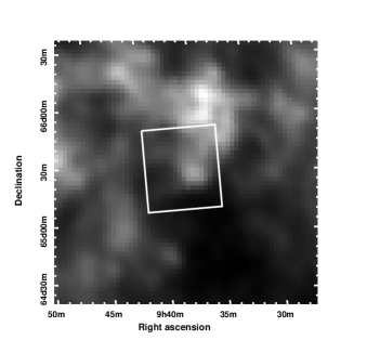
Figure 1: Optical field superimposed on the $IRAS$/DIRBE 100$\micron$ map. The solid square represents the observed field. The brightest point of the 100$\micron$ map corresponds to the center of CO emission from molecular cloud MBM32 (Magnani et al. 1985).

2.2 Data processing

The data reduction was performed in a standard manner, including overscan subtraction, bias subtraction, and flat-fielding with dome-flat, using the IRAF software package. The flux calibration was obtained from nearly 1,000 stars in a range of 15 - 19 mag which are listed in the Sloan Digital Sky Survey (SDSS) Data Release 8 photometric catalog (Aihara et al., 2011). The SDSS magnitudes (psfMag) are transferred to the BVR magnitudes (Jester et al., 2005), and then correlated against instrumental magnitudes to derive the zero-points. The SExtractor software package (Bertin & Arnouts, 1996) was used with a circular aperture of 8^′′ radius. The uncertainty in the zero-points is estimated to be 0.01 - 0.02 mag. The systematic errors introduced through the conversion of magnitudes are approximately 0.03 mag.

2.2.1 Masking of stars and galaxies

In order to obtain the diffuse component, we masked stars and galaxies in the images. Our masking procedure is as follows. First, we detected all the discrete sources that exceed 1.5 $\sigma$ of the local background in more than three contiguous pixels using SExtractor with parameters DETECT_THRESH = 1.5 and DETECT_MINAREA = 3. Second, from the detected bright stars, we derived point spread functions (PSFs) by fitting a Moffat function $I=I_{0}[1+(r/\alpha)^{-2}]^{-\beta}$ (Moffat 1969), where $I_{0}$ is the intensity at the center of the stellar image and $\alpha$ and $\beta$ are the fitting parameters depending on the seeing. Figure 2 shows the radial profiles of bright unsaturated stars along with the best-fit curves. Adopting these best-fit curves as the PSF templates, every unsaturated star is masked with a circle with the radius where the count level is equal to 1/10 $\sigma$ of the local background count level. Saturated stars, magnitudes of which are supposed to be underestimated, are masked with a sufficiently large radius such as five or ten times larger than the masking radius estimated by using the flux value and the PSF for an unsaturated star. The unmasked and masked images are presented in Figure 3 and Figure 4, respectively. The fractions of masked areas in B, g, V, and R images are 17%, 31%, 19%, and 35%, respectively.

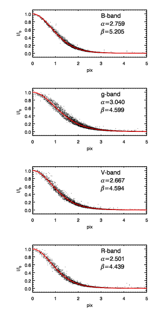
Figure 2: The scaled radial profiles of stellar images. Dots represent the normalized fluxes of approximately hundred stars for each band. The red lines are the best fit of a Moffat function; $I=I_{0}[1+(r/\alpha)^{-2}]^{-\beta}$.

2.2.2 Aperture correction

In the flux calibration of the surface brightness of extended sources, as extensively discussed by Bernstein et al. (2002) and Mattila (2003), one must compensate for the flux that is scattered and diffracted into the aperture. Here we introduce the aperture correction factor, $T_{A}$, which is the fraction of the flux from a point source within the aperture. The flux from the point source, $F(\lambda)$, in units of Jy is given by

$$F(\lambda)={Q(\lambda)\over T_{A}(\lambda)}C(\lambda),$$ (1)

where $C(\lambda)$ is the signal counts within the aperture in instrumental units (ADU), $Q(\lambda)$ the sensitivity function in units of Jy ADU^-1. Because $F(\lambda)$ is known and $C(\lambda)$ is measured, we can only derive $Q^{\prime}(\lambda)$= $Q(\lambda)$ /$T_{A}(\lambda)$, but not $Q(\lambda)$ and $T_{A}(\lambda)$ independently. In case of an extended source, no flux is lost; the flux lost from the aperture $1-T_{A}(\lambda)$ is compensated for by the flux scattered in, from the outside the aperture. Therefore, the brightness of the extended source $S(\lambda)$ in units of Jy sr^-1 is simply given as

$$S(\lambda)={Q(\lambda)\over\Omega}C(\lambda)={Q^{\prime}(\lambda)T_{A}(\lambda)\over\Omega}C(\lambda),$$ (2)

where $\Omega$ is the solid angle of the aperture in units of steradians. In the above equation, $S(\lambda)$ is obtained once $T_{A}(\lambda)$ is given.

The flux loss calculated from the fitted Moffat function is negligible; $T_{A}(\lambda)=0.994$. However, King (1971) pointed out that outside the central part of the profile, which is represented by a Gaussian or Moffat function, there is a more slowly declining halo or aureole. The aureole has a profile of an inverse-square law that extends out from the central part by a factor of 1000 in angular distance, and contains about 5% of the star’s light. Similar results are presented by several authors (Mattila 2003 and references therein). Even higher aureole energy fractions of $\sim 10\%$ are reported in some cases (Capaccioli & de Vaucouleurs 1983; Uson et al. 1991). Here, we adopt the aperture correction factor $T_{A}$ = 0.95$\pm$0.05 as a compromise.

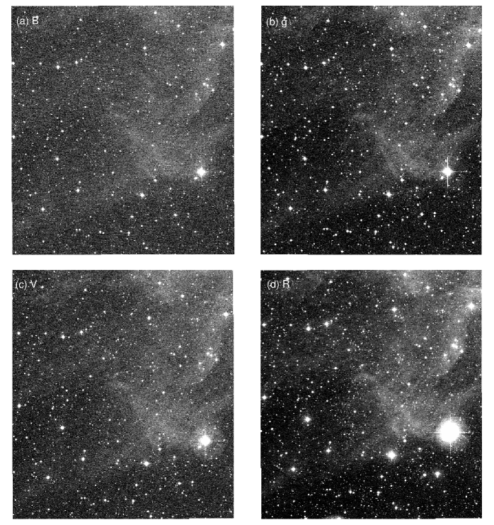
Figure 3: The optical images in B-band (a), g-band (b), V-band (c), and R-band (d). North is up, east to the left. The field is approximately 45′$\times$ 40′, slightly smaller the field of view of instrument due to using dithering.

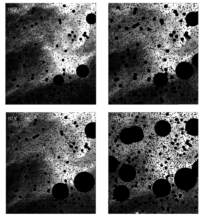
Figure 4: Same as for Figure 3, but for the masked optical images.

Table 1: Observations and errors.

	$\lambda_{center}$	$\sigma(\lambda)$	Obs. date
Band	($\micron$)	(kJy sr-1)	(UT)
B	0.44	0.48	2011-02-04
g	0.49	0.39	2011-04-03
V	0.55	0.79	2011-02-21
R	0.65	0.39	2012-02-21
$IRAS$/DIRBE	100	0.3 $\times 10^{3}$

3 Analysis and Results

Figure 5 plots the intensity of diffuse optical light, $S_{\nu}(\lambda)$, as a function of 100$\micron$ intensity, $S_{\nu}(100\micron)$. $S_{\nu}(100\micron)$ is taken from the $IRAS$/DIRBE 100$\micron$ map where the zodiacal light, stars, and galaxies are subtracted. We reduced the resolution of the optical images to the same resolution as the $IRAS$/DIRBE 100$\micron$ map (2$\farcm$372 $\times$ 2$\farcm$372) by averaging approximately 9,000 optical pixels. Considering the seeing induced correlation, approximately 10 optical pixels constitute one independent data point. Thus, in the course of smoothing, the optical measurement errors are reduced by a factor of 30 as if averaging 900 independent data points. The mean one $\sigma$ error per smoothed pixel, $\sigma(\lambda)$, of the smoothed star-masked images is summarized in Table 1. Finally, we obtained 385, 336, 384, and 309 independent data points at $B,g,V$, and $R$, respectively.

Figure 5 shows that $S_{\nu}(\lambda)$ clearly correlates with $S_{\nu}(100\micron$) at all the bands. We now fit to the data a linear function defined as:

$$S_{\nu}(\lambda)=a(\lambda)+b(\lambda)S_{\nu}({100\micron})$$ (3)

where the slope parameter at wavelength $\lambda$ is $b(\lambda)$ = $\Delta S_{\nu}({\lambda})/\Delta S_{\nu}(100\micron)$, and the constant parameter $a(\lambda)$ represents components independent of the Galactic diffuse optical light (i.e., atmospheric airglow, zodiacal light, and any other light such as the COB). Note that $\lambda$ is $B,g,V,$ or $R$ for our broadband system, and $a(\lambda),b(\lambda)>0$.

To perform a minimum $\chi^{2}$ analysis with the effective variance method (Orear, 1982) which can take into account both x and y errors, we need to know the standard deviation, $\sigma(100\micron$), which is not explicitly estimated by SFD98. We thus carried out simulations by generating noiseless data points which follow equation (3) with given $a(\lambda)$ and $b(\lambda)$, and adding Gaussian random errors to these points. The noiseless 100$\micron$ data range from MIN(100$\micron$) to 8 MJy sr^-1 with a frequency distribution $\propto S_{\nu}(100\micron)^{-n}$. At the low intensity end of $S_{\nu}(\lambda)$ in Figure 5, the correlation appears to be truncated suddenly because of the large scatter of the 100$\micron$ data. The center of the truncated boundary along the $S_{\nu}(100\micron$) axis is located around 1.8 MJy sr^-1. So, we set MIN(100$\micron$) = 1.8 MJy sr^-1. This was confirmed and justified by changing MIN(100$\micron$) in the simulations. While $\sigma(\lambda)$ is taken from Table 1, $\sigma(100\micron$) is a parameter to be determined in the simulations. We find that a combination of $n=2$ and $\sigma(100\micron$) = 0.3 - 0.4 MJy sr^-1 reasonably reproduces the correlation and the frequency distribution as a function of $S_{\nu}(100\micron$).

The bottom panel of Figure 5 shows the simulated data at the $g$-band along with the linear function recovered from the $\chi^{2}$ minimum analysis as well as the assumed linear function to generate the mock data points. The top and middle panels plot the observed data along with the recovered linear function. $a(\lambda)$ and $b(\lambda)$ are listed in Table 2.

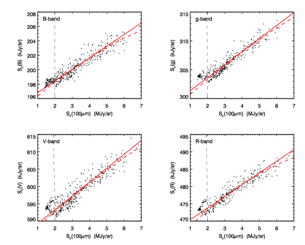
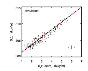
Figure 5: Correlation of the intensity of the diffuse optical light against 100$\micron$ intensity. The top and middle panels show the measured data. The red solid lines represent the linear functions recovered from the $\chi^{2}$ minimum analysis, while the red dashed lines represent the quadratic functions. In case of a quadratic function, the fit is limited to the data points with $S_{\nu}(100\micron$) $\geq$ 2.0 MJy sr^-1 (right to the vertical dash line); all the data points are used to fit the linear functions. The bottom panel shows the mock data. The black dashed line represents the linear function assumed in the simulations, while the red line represents the recovered function.

Table 2: DGL model parameters.

	$S_{\nu}(\lambda)=a(\lambda)+b(\lambda)S_{\nu}({100\micron})$			$S_{\nu}(\lambda)=a^{Q}(\lambda)+b^{Q}(\lambda)S_{\nu}({100\micron})+c^{Q}(\lambda)S_{\nu}({100\micron})^{2}$
	$a(\lambda)$	$b(\lambda)$		$a^{Q}(\lambda)$	$b^{Q}(\lambda)$	$c^{Q}(\lambda)$
Band	(kJy sr-1)	($\times 10^{-3}$)		(kJy sr-1)	($\times 10^{-3}$)	([kJy sr-1]${}^{-1}\times 10^{-6}$)
B	195.23 $\pm$ 0.12	1.61 $\pm$ 0.11		194.28 $\pm$ 0.50	2.17 $\pm$ 0.28	-0.08 $\pm$ 0.04
g	299.16 $\pm$ 0.16	2.25 $\pm$ 0.14		298.00 $\pm$ 0.60	2.80 $\pm$ 0.34	-0.07 $\pm$ 0.04
V	585.27 $\pm$ 0.46	4.00 $\pm$ 0.28		583.67 $\pm$ 1.02	4.74 $\pm$ 0.56	-0.11 $\pm$ 0.07
R	467.06 $\pm$ 0.22	3.37 $\pm$ 0.21		463.61 $\pm$ 0.91	5.23 $\pm$ 0.47	-0.24 $\pm$ 0.06

4 Discussion

4.1 Variations in slope parameter $b(\lambda)$

To explore the variations in slope parameter $b(\lambda)$, we compiled $b(\lambda)$ values from the literature into a sample which is given in Table 3. Figure 6 compares the data in this sample with model predictions. For the data points in the sample, the $IRAS$/DIRBE 100 $\micron$ maps are used in Witt et al. (2008), Matsuoka et al. (2011), Brandt & Draine (2012), and this work, while early work, namely Laureijs et al. (1987), Guhathakurta & Tyson (1989), Paley et al. (1991), and Zagury et al. (1999) used the original IRAS 100$\micron$ maps. The optical data are a collection of heterogeneous samples which were taken with different techniques and analyzed using different methods. The broadband data taken from the literature are: fields towards diffuse cloud Lynds 1642 studied by Laureijs et al. (1987), four diffuse clouds ($|b|\geq 25$°) at $B_{J}$, R, and I by Guhathakurta & Tyson (1989), a compact high-latitude source at B, V, and R by Paley et al. (1991), a molecular cloud MCLD123.5+24.9 by Zagury et al. (1999), and four high-latitude molecular clouds (MBM 30, 32, 41A, and 41D) at B, G, R, and I by Witt et al. (2008). The data studied by Matsuoka et al. (2011) were taken beyond the zodiacal dust zone with the Pioneer 10/11 Imaging Photopolarimeter(IPP) at $B$ and $R$ in regions with $S_{\nu}(100\micron$) $\leq$ 3 MJy sr^-1 at Galactic latitude $|b|>35\arcdeg$, covering about a quarter of the whole sky. The spectrum by Brandt & Draine (2012), labeled ”Full Sky Continuum” in their Figure 3, are obtained by analyzing the optical spectra of nearly 90,000 blank-sky spectra from the Sloan Digital Sky Survey (SDSS), the weighted regional coverage of which is concentrated at intermediate Galactic latitudes $|b|=30\arcdeg\sim 45\arcdeg$. Their spectrum has a large uncertainty in the flux calibration due to their analyzing method. The spectra plotted in Figure 6 are scaled with their preferred bias factor of 2.1. In the case where more than one cloud is published in a single paper, the average $b(\lambda)$ value is plotted with the standard deviation. As can be seen, $b(\lambda)$ varies by a factor of 3 - 4.

In the following subsections, we explore possible causes of the large $b(\lambda)$ scatter by examining the effects of optical depth, dust albedo, dust temperature and the forward-scattering characteristic of dust grains coupled to the non-isotropic interstellar radiation field (ISRF).

Table 3: Correlation slopes $b(\lambda)$ for high-latitude clouds or fields.

Reference	$b(\lambda)^{\dagger}$	$\lambda_{center}$	$S_{\nu}(100\micron)$ range	$b(R)/b(B)$
Clouds or fields	($\times 10^{-3}$)	(µm)	(MJy sr-1)
This work
MBM32($l=147,b=41$)	1.6 $\pm$ 0.1	0.44	1 - 7	2.1
	2.3 $\pm$ 0.1	0.49
	4.0 $\pm$ 0.3	0.55
	3.4 $\pm$ 0.2	0.65
Laureijs et al. 1987
Lynds1642($l=211,b=-38$)	2.2 $\pm$ 0.3	0.47	1 - 13
Guhathakurta et al. 1989
ir1($l=174,b=-42$)	0.4	0.45	7 - 18	3.2
	1.2	0.65
ir2($l=235,b=37$)	1.1	0.45	3 - 7	2.0
	2.2	0.65
ir3($l=38,b=45$)	2.6	0.45	3 - 9	1.7
	4.4	0.65
	6.0	0.90
Paley et al. 1991
CTI cirrus cloud($l=104,b=-32$)	4.5 $\pm$ 0.3	0.44	2.5	2.3
	8.5 $\pm$ 0.8	0.55
	11.0 $\pm$ 1.0	0.70
Zagury et al. 1999
MCLD123.5+24.9($l=124,b=25$)	2.4 $\pm$ 0.1	0.45	5 - 8	1.8
	4.3 $\pm$ 0.1	0.65
	3.0 $\pm$ 0.1	0.90
Witt et al. 2008
Derived from 4 clouds($90\leq l\leq 147,38\leq b\leq 41$)	2.1 $\pm$ 0.1	0.46	1 - 8	2.0
	3.3 $\pm$ 0.4	0.53
	4.2 $\pm$ 0.7	0.63
	2.7 $\pm$ 0.7	0.83
Matsuoka et al. 2011
1/4 of the entire sky ($|b|>35^{\circ}$)	2.1 $\pm$ 0.1	0.44	1 - 3	2.2
	4.6 $\pm$ 0.1	0.64
Brandt et al. 2012
SDSS spectra ($30\leq b\leq 45$)	1.2 $\pm$ 0.1	0.45	1 - 10	1.9
	2.3 $\pm$ 0.1	0.65

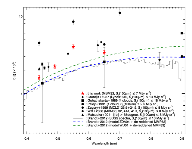
Figure 6: The correlation slopes $b(\lambda)$ = $\Delta S_{\nu}(\lambda)/\Delta S_{\nu}(100\micron)$ as a function of wavelengths.

4.1.1 Optical depth and dust albedo

The correlation in Figure 5 may appear to be linear. However, as we discuss below, linear correlations would not be expected in the case where the optically thin limit is not applicable, and significant changes in the optical depth along the sightline would cause large variations in $b(\lambda)$ from cloud to cloud.

Figure 7 depicts $b(\lambda)$ as a function of $S_{\nu}^{ave}(100\micron$) in two ranges of the effective broadband wavelengths, namely the blue range(0.43 - 0.48 µm) and the red range (0.62 - 0.66 µm). $S_{\nu}^{ave}(100\micron$) refers to the representative average of the lowest and highest values of the $S_{\nu}(100\micron$) range in which $b(\lambda)$ are derived by assuming a linear function. For the three clouds published in Guhathakurta & Tyson (1989), the plotted $b(\lambda)$ values refer to individual clouds, not averaged values. The figure clearly shows that the $b(\lambda)$ decreases as $S_{\nu}^{ave}(100\micron$) increases, indicating that a significant portion of the reason for the large $b(\lambda)$ scatter seen in Figure 6 can be attributed to this $b(\lambda)$ - $S_{\nu}^{ave}(100\micron$) anti-correlation.

Accordingly we propose a correction to equation (3) as $b(\lambda)$ = $b^{0}(\lambda)+b^{1}(\lambda)S_{\nu}(100\micron)$, or $S_{\nu}(\lambda)$ = $a(\lambda)$ + $[b^{0}(\lambda)+b^{1}(\lambda)S_{\nu}(100\micron)]S_{\nu}({100\micron})$. Then, $S_{\nu}(\lambda)$ has a quadratic term as follows:

$$S_{\nu}(\lambda)=a^{Q}(\lambda)+b^{Q}(\lambda)S_{\nu}({100\micron})+c^{Q}(\lambda)S_{\nu}({100\micron})^{2},$$ (4)

where $b^{Q}(\lambda)>0$ and $c^{Q}(\lambda)<0$. While the correlation in Figure 5 appears to be linear, the actual fact is that the correlation is non-linear, but this is hidden by the prevailing noise. Since the quadratic term $c^{Q}(\lambda)S_{\nu}({100\micron})^{2}$ is negative, this would explain why the correlation of the $Pioneer$ data deviates below the best-fit linear function at the bright end of 100$\micron$ emission (Matsuoka et al., 2011). We performed a minimum $\chi^{2}$ analysis with the effective variance method to fit the quadratic function to our data. As can be seen in Table 2 and Figure 5, the derived constant parameter of a quadratic function $a^{Q}(\lambda)$ is smaller than that of a linear function $a(\lambda)$ at all the photometric bands. Thus, this negative quadratic term would be important for the separation of the COB from the diffuse optical light, reducing the DGL intensity at which $S_{\nu}(100\micron$) is equal to the Cosmic 100$\micron$ background intensity.

The origin of the quadratic term could be attributed to the fact that our sample directions are not optically thin, but translucent or thick. Figure 8 illustrates the relation between reddening $E(B-V)$ and 100$\micron$ emission at the peak of 100µm emission for our clouds, where $E(B-V)$ is taken from the $IRAS$/DIRBE reddening map. If typical extinction curve ($R_{V}=A_{V}/E(B-V)=3.1$) is assumed, the 100$\micron$ brightness per unit of visual extinction is $S_{\nu}(100\micron$)/$A_{V}$ = 8 - 15 MJy sr^-1 mag^-1. Our sample ranges from $S_{\nu}(100\micron$) = 3 to 18 MJy sr^-1, corresponding $A_{V}$ = 0.16 - 2.0 mag. Thus, dust absorption along the sightline should be taken into account.

To illustrate the effect of extinction along the sightline, as fully discussed in the Appendix, we consider a simple model where a plane-parallel dust slab is illuminated by the monochromatic starlight from the back. The $b(\lambda)$ is expressed as

$$b(\lambda)\propto\exp[-(1-\omega)\tau][1-\exp(-\omega\tau)]/\{1-\exp[-(1-\omega)\tau]\},$$ (5)

where $\omega$ is the albedo.

Equation (5) implies that $b(\lambda)$ depends on the optical depth and the albedo, but not on the ISRF intensity. In Figure 7, we plot equation (5) with a single constant value of proportionality, $X$, both for the left and right panels, assuming $S_{\nu}(100\micron)/A_{V}=$ 10 MJy sr^-1 mag^-1. $X$ is set to an appropriate value by eye. The three lines depict the relation for albedo $\omega_{V}$ of 0.6, 0.7, and 0.8 from bottom to top. Figure 7 suggests that a range of $A_{V}$ = 0.16 - 2.0 mag could change the $b(\lambda)$ strength by a factor of 2 - 3 while keeping $\omega$ constant. It also indicates that the $A_{V}$ range alone cannot explain the full range of the $b(\lambda)$ scatter. If the albedo becomes greater as the optical depth becomes smaller, then the full range of the $b(\lambda)$ scatter could be explained in terms of the optical depth effect coupled to variations in albedo. However, this case is not likely, because small-size dust grains, which have smaller albedo than large ones(e.g. Draine 2003), are expected in smaller optical depth regions according to the theory of grain growth.

Two smooth curves in Figure 6 are synthesized spectra for $\tau_{V}$ = 0.15 by Brandt & Draine (2012), adopting the ISRF spectrum by Mathis et al. (1983) combined with a simple plane-parallel galaxy model and two dust models from Zubko et al. (2004) and Weingartner & Draine (2001) (hereafter ZDA04 and WD01 models). The models underestimate $b(\lambda)$ by a factor of 2. There would be two possible explanations for this. One is a deficiency in UV photons compared to the assumed spectrum of the ISRF; the dust temperature is low and $b({\lambda})$ thus increases where the dust grains are illuminated by a small number of UV photons(see Figures 9 and 10 in Brandt & Draine 2012). The other is that the albedo is greater than assumed in the models, because Figure 7 and equation (5) imply that the $b(\lambda)$ strength is doubled if $\omega$ increases by 20%; for example, $\omega_{V}$ to be 0.8 instead of a standard Milky Way value of 0.67 at V (Draine, 2003). If this is the case, more large grains are needed than in the ZDA04 and WD01 models, because large grains are efficient scatters of light.

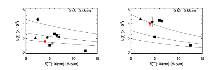
Figure 7: The left panel plots the correlation slopes $b(\lambda)$ as a function of $S_{\nu}^{ave}(100\micron$) for the blue range (0.43 to 0.48 µm). $S_{\nu}^{ave}(100\micron$) refers to the representative average of the lowest and highest values of the $S_{\nu}(100\micron$) range in which $b(\lambda)$ is derived by fitting a linear function. Spectroscopic data are averaged over this range. The right panel is the same as for the left panel but for the red range (0.62 to 0.66 µm). The legend for the points is the same as in Figure 6, except for the crosses which are the averaged spectroscopy data from Brandt & Draine (2012). The lines represent the relation expected from equation (5) for albedos $\omega_{V}=0.6,0.7,$ and $0.8$ from lower to upper.

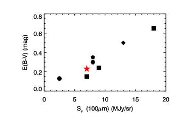
Figure 8: $E(B-V)$ as a function of $S_{\nu}(100\micron$) for the peak of 100µm emission in the cloud. The legend for the points is the same as in Figure 6.

4.1.2 Dust Temperature

Another possible cause of the large $b(\lambda)$ scatter is variations in dust temperature. Higher dust temperature increases the intensity of the 100µm emission and, as a consequence, it would decrease the $b(\lambda)$. The temperature dependence of the resulting 100µm radiation is $\sim T^{5.8}$ at 18K (Brandt & Draine, 2012). However the real situation is not so simple. The temperature of 100µm-emitting dust grains, i.e. large grains, is determined by the balance between incoming energy from the illuminating radiation to the grains and the outgoing infrared thermal energy. One can increase the temperature of the grains by increasing the UV component of the ISRF while leaving the optical intensity of the ISRF the same. That would leave the optical DGL intensity the same but increase the 100µm intensity. However, if the optical intensity of the ISRF changes, it also changes the intensity of the DGL. Thus, the increment of $b(\lambda)$, e.g the ratio of increment of the DGL and that of the 100µm emission, depends intricately on the spectral energy distribution and the non-isotropy of the ISRF. Lehtinen et al. (2007) showed that the dust emissivity, which is measured from the ratio of far-IR optical depth to visual extinction $\tau$(far-IR)/$A_{V}$, decreases as a function of dust temperature, and the higher temperature dust does not necessarily mean the higher surface brightness at 100µm. They concluded that the emissivity variations are caused by the variations in the absorption cross section of dust in the far-IR, or the grain size distribution.

In our sample, we do not see any convincing correlation between $b(\lambda)$ and dust temperature $T$ as shown in Figure 9. The plotted dust temperatures are taken from the $IRAS$/DIRBE temperature map. The $T^{5.8}$ dependence of the 100µm intensity causes an increase by a factor of about 1.7 over a temperature range from 16K to 17.5K shown in the data of Figure 9. However, the ratio of $\tau$(far-IR)/$A_{V}$ declines with increasing temperature, and the effective increase in $S_{\nu}(100\micron$) would become lower than 1.7. This may explain why the data of Figure 9 do not lead to any discernible trends. As a caveat, it should be noted that the $IRAS$/DIRBE temperature map is severely limited by the angular resolution of DIRBE of $\sim$ 1 degree. Thus, this map is not capable of correctly reflecting the temperature variations across cloud structures with scales much smaller than the DIRBE resolution. Further exploration of the $b(\lambda)$ dependence on the dust temperature requires far-IR data with higher resolution such as those from the Akari all sky survey. Such analysis is beyond the scope of this paper.

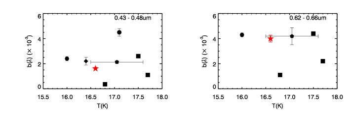
Figure 9: The left panel plots the correlation slopes $b(\lambda)$ as a function of $T_{dust}$ for the blue range of the effective broadband wavelengths. The right panel is the same as for the top panel but for the red range. The legend for the points is the same as in Figure 6. The horizontal error bars are represent their temperature ranges among the clouds.

4.1.3 Forward-scattering characteristic of dust grains

Another possible cause of the large $b(\lambda)$ scatter is the effect of the forward-scattering characteristic of dust grains. The ISRF is non-isotropic because of the stellar concentration toward the Galactic disk. The scattering efficiency in the direction towards the observer is coupled to this non-isotropy through the forward-scattering phase function of scattering grains. This effect is maximized for the geometric configuration explored by Jura (1979) and Stark (1995). The latitude dependence of surface brightness of a cloud at high latitude was studied, employing the Henyey & Greenstein (1941) approximation for the scattering phase function. In this model, it is assumed that a cloud is illuminated by an infinite homogeneous disk. The observer is located in the plane, and the cloud is located above the plane. The numerical results by Jura (1979) show that the surface brightness of a cloud $S$ is written as

$$S\propto 1-1.1g\sqrt{\sin|b|}$$ (6)

where $g$ is the asymmetry factor of the phase function and $b$ the Galactic latitude. For strong forward scattering, $g\sim 1$; for isotropic scattering, $g\sim 0$. This equation shows that the brightness of the scattered light is significantly changed with the latitude of the cloud. Adopting a typical asymmetry factor $g\sim 0.75$, the intensity of the scattered light at $b=30\arcdeg$ is 2-3 times larger than that of at $b=90\arcdeg$. This model assumes that all radiation sources, i.e. stars, are located just in a plane, however, this is not the case. In fact, the mean vertical height of high-latitude clouds is $\sim 150$ pc (Magnani et al., 1996) and that of the stellar disk is $\sim 300$ pc (Bahcall & Soneira, 1980; Gilmore & Reid, 1983). Thus, the geometry used in the model of Jura (1979) is extreme. It would be more natural to assume that a significant portion of stars are located behind the high-latitude clouds.

To examine the effectiveness of the forward-scattering characteristic of dust grains, we present Figure 10, illustrating $b(\lambda)$ as a function of Galactic latitude $|b|$ (upper panels) and longitude $|l|$ (lower panels). In upper panels, we may see a correlation between the $b(\lambda)$ and the Galactic latitude $|b|$ in the blue range, but no correlation in the red range. There are no $b(\lambda)$ dependency on the longitude $|l|$ at all. For comparison, equation (6) with $g=0.75$ is plotted in upper panels of Figure 10. The absolute value of the equation is determined by eye to fit the observed data. The $b(\lambda)$ variation in the blue range seems to be partly explained in terms of the forward-scattering. Then, why are there no correlations in the red range? A possible cause could be a difference in the distribution of blue stars (i.e., effective emitter of blue light) and red stars (i.e., effective red light emitter). Blue young stars are more concentrated towards the Galactic plane than red old stars and the $g$ value at the blue range is greater than the red range in dust models (e.g, Draine 2003). Thus, the effect of the forward-directed scattering phase function would be more efficient in the blue range than in the red range.

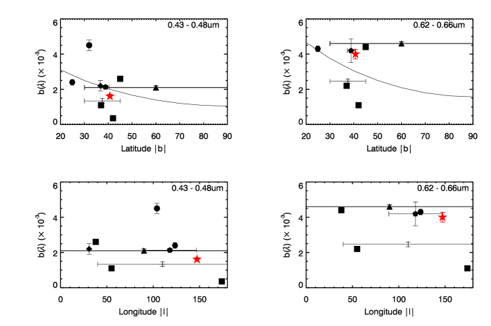
Figure 10: The upper panels plot the correlation slopes $b(\lambda)$ as a function of Galactic latitude $|b|$, and the lower panels the correlation slopes $b(\lambda)$ as a function of Galactic longitude $|l|$. The left and right panels are for the blue range of the effective broadband wavelengths and for the red range, respectively. The line solid curve represents the prediction from equation (6), which is derived by assuming models where the effectiveness of the forward-scattering characteristic of dust grains is maximized. The legend for the points is the same as in Figure 6. The horizontal error bars are represent coordinate ranges.

4.2 Extended red emission

Extended red emission (ERE) is observed as an excess in the 5000-9000Å  spectral range in the ISM. It is suggested that ERE is the result of an interaction of far-UV photons with interstellar dust (Witt & Schild, 1985; Darbon et al., 1999; Witt et al., 2006). ERE is observed in reflection nebulae (Witt et al., 1984; Witt & Schild, 1988; Witt & Boroson, 1990), HII regions (Perrin & Sivan, 1992), and planetary nebulae (Furton & Witt, 1990, 1992). In the diffuse ISM, such as high latitude clouds, some authors favor the presence of ERE in the diffuse optical light (e.g., Guhathakurta & Tyson 1989; Gordon et al. 1998; Witt et al. 2008; Matsuoka et al. 2011), while others suggest the absence of ERE (Zagury et al. 1999; Zagury 2006) based on broadband observations. The cloud observed by Zagury et al. (1999) and Zagury (2006) is illuminated by the nearby star Polaris (F7 Ib). The optical surface brightness of the cloud is dominated by scattered light of Polaris, but this star is not blue enough to emit sufficient far-UV photons for ERE excitation (private communications with the anonymous referee; see section 6.4 of Lehtinen & Mattila (2013) for further discussion). Thus, it would be natural for them to miss ERE. Carrying out spectroscopy of the diffuse optical light toward a high latitude cloud, Szomoru & Guhathakurta (1998) claimed to detect ERE peaking at 6000Å, which is blue-shifted compared with 8000Å for HII regions and 7000Å for reflection nebulae and planetary nebulae. On the other hand, the more recent spectroscopic study by Brandt & Draine (2012) cannot find any evidence of ERE.

There is some confusion in the DGL models, which are sometimes used for the claim of ERE detection; ERE is detected, if the observed diffuse optical light is redder than predicted by the model, and vice verse. Here we introduce the $b(R)/b(B)$ value, which is a measure of the redness of the diffuse optical light. As indicated in Table 3, measured $b(R)/b(B)$ values are typically $\sim 2$. Models by Witt & Schild (1985), Guhathakurta & Tyson (1989), and Bernstein et al. (2002) predict $b(R)/b(B)\sim 1.4$, which is bluer than the measured values $b(R)/b(B)\sim 2$, supporting the presence of ERE in the diffuse optical light. In contrast, Gordon et al. (1998) predicted $b(R)/b(B)\sim 1.9$, using the Witt-Petersohn DGL model(WP model; Witt & Petersohn 1994; Witt et al. 1997), an advanced Monte Carlo multiple scattering model utilizing the actual Galactic radiation field and realistic dust scattering properties. Brandt & Draine (2012) also predicted $b(R)/b(B)\sim 1.9-2.0$ using their scattering DGL models(ZDA04 and WD01). These are consistent with the observed values without ERE. However, the observed values deduced from $PIONEER$10/11 data from the high-latitude regions by Gordon et al. (1998) are $b(R)/b(B)\sim 3.2$, which is higher than other observed values, and still redder than the models.

It is emphasized that $b(\lambda)$ in this work on cloud MBM32 in Figure 6 has an excess at the $V$-band and favors ERE in the diffuse optical light; $b(\lambda)$ rises from B to V faster than the models, seems to peak around 6000 Å  and decreases towards long wavelengths. Such a characteristic is expected from the models in which scattered DGL is combined with ERE.

5 Summary

We have conducted B, g, V, and R-band imaging in a $45\arcmin\times 40\arcmin$ field containing part of the high Galactic latitude translucent cloud MBM32, and correlated the intensity of the diffuse optical light $S_{\nu}(\lambda)$ with that of 100$\micron$ emission $S_{\nu}(100\micron)$. $S_{\nu}(100\micron$) ranges from 1.4 to 7.0 MJy sr^-1 in the field. A minimum $\chi^{2}$ analysis is applied to fit a linear function to the measured correlation and to derive the slope parameter $b(\lambda)$ of the best-fit linear function.

Compiling a sample by combining our $b(\lambda)$ and published ones, we showed that the $b(\lambda)$ strength varies from cloud to cloud by a factor of 4. We also found that $b(\lambda)$ decreases as $S_{\nu}(100\micron)$ increases in the sample. To incorporate this $b(\lambda)$ - $S_{\nu}(100\micron)$ relation, we proposed that a non-linear correlation including a negative quadratic term of $S_{\nu}(100\micron)^{2}$ be fitted to the measured correlation.

We explored possible causes of the large $b(\lambda)$ scatter by examining the effects of the optical depth, dust albedo, dust temperature and the forward-scattering characteristic of dust grains coupled to the non-isotropic interstellar radiation field(ISRF). The variation of optical depth, which is $A_{V}$ = 0.16 - 2.0 in the sample, can change $b(\lambda)$ by a factor of 2 - 3 while keeping the albedo, $\omega$, constant. This indicates that the $A_{V}$ range alone cannot explain the full range of the $b(\lambda)$ scatter. Our finding of a correlation between the $b(\lambda)$ and Galactic latitude $|b|$ in the blue range (0.43 - 0.48µm) would imply that there would be some contribution to the $b(\lambda)$ scatter from the effect of the forward-scattering characteristic of dust grains coupled to the non-isotropic interstellar radiation field(ISRF).

The models by Brandt & Draine (2012) underestimate $b(\lambda)$ by a factor of 2. There would be two possible explanations for this. One is a deficiency in UV photons compared to the assumed spectrum of the ISRF, because fewer UV photons result in lower dust temperature, which increases $b({\lambda})$. The other is that the albedo is greater than assumed in the models. If this is the case, a greater number of larger grains are needed in the models, because large grains are more efficient scatterers of light.

Our $b(\lambda)$ spectrum favors the presence of extended red emission(ERE) in the diffuse optical light; $b(\lambda)$ rises from B to V faster than the models, seems to peak around 6000 Å  and decreases towards longer wavelengths. Such characteristic is expected from the models in which the DGL is combined with ERE.

Appendix A Radiative transfer in a dusty slab

Here we consider a simple model where a plane-parallel dust slab is illuminated from the back by monochromatic starlight at optical wavelength $\lambda$. We measure optical depth $\tau$ inward toward the plane-parallel slab. Light is produced along a sightline by the scattering of the illuminating starlight and from scattered light in the slab. Here, we assume complete forward-scattering for simplicity. The contribution of an element with optical depth from $\tau$ to $\tau+d\tau$ to the scattered light and the starlight are given by

$$dI_{\nu,sca}(\tau)=[I_{\nu,star}(\tau)+I_{\nu,sca}(\tau)]\omega d\tau-I_{\nu,sca}(\tau)d\tau$$ (A1)

$$dI_{\nu,star}(\tau)=-I_{\nu,star}(\tau)d\tau$$ (A2)

where $I_{\nu,sca}(\tau)$ and $I_{\nu,star}(\tau)$ are the specific intensity of the scattered light and the starlight, respectively, $\omega$ is the albedo. Then the solution of $I_{\nu,sca}(\tau)$ is given by

$$I_{\nu,sca}(\tau)=I_{\nu,star}(0)\exp[-(1-\omega)\tau][1-\exp(-\omega\tau)].$$ (A3)

The far-infrared(IR) luminosity $L(IR)$ comes from thermal emission from dust grains which absorb the starlight and the scattered light. The contribution of an element to $L(IR)$ is given by

$$dL_{\nu,IR}(\tau)\propto[I_{\nu,star}(\tau)+I_{\nu,sca}(\tau)](1-\omega)d\tau.$$ (A4)

By integrating this equation, we have

$$L_{\nu,IR}(\tau)\propto I_{\nu,star}(0)\{1-\exp[-(1-\omega)\tau]\}.$$ (A5)

The conversion of the total IR luminosity to the 100$\micron$ luminosity is $L(100\micron$) = 0.52$L(IR)$, which is applicable for models from 0.5 to 1.5 times the local ISRF intensity (Brandt & Draine, 2012). Thus we have

$$b(\lambda)\propto\exp[-(1-\omega)\tau][1-\exp(-\omega\tau)]/\{1-\exp[-(1-\omega)\tau]\}$$ (A6)

where $b(\lambda)$ is the intensity of the scattered light at wavelength $\lambda$ relative to the intensity of 100$\micron$ emission.

References

- Aihara et al. (2011) Aihara, H., Allende Prieto, C., An, D., et al. 2011, ApJS, 193, 29
- Bahcall & Soneira (1980) Bahcall, J. N., & Soneira, R. M. 1980, ApJS, 44, 73
- Beichman (1987) Beichman, C. A. 1987, ARA&A, 25, 521
- Bernstein et al. (2002) Bernstein, R. A., Freedman, W. L., & Madore, B. F. 2002, ApJ, 571, 56
- Bertin & Arnouts (1996) Bertin, E., & Arnouts, S. 1996, A&AS, 117, 393
- Brandt & Draine (2012) Brandt, T. D., & Draine, B. T. 2012, ApJ, 744, 129
- Capaccioli & de Vaucouleurs (1983) Capaccioli, M., & de Vaucouleurs, G. 1983, ApJS, 52, 465
- de Vries & Le Poole (1985) de Vries, C. P., & Le Poole, R. S. 1985, A&A, 145, L7
- Darbon et al. (1999) Darbon, S., Perrin, J.-M., & Sivan, J.-P. 1999, A&A, 348, 990
- Draine (2003) Draine, B. T. 2003, ARA&A, 41, 241
- Elvey & Roach (1937) Elvey, C. T., & Roach, F. E. 1937, ApJ, 85, 213
- Furton & Witt (1990) Furton, D. G., & Witt, A. N. 1990, ApJ, 364, L45
- Furton & Witt (1992) Furton, D. G., & Witt, A. N. 1992, ApJ, 386, 587
- Gilmore & Reid (1983) Gilmore, G., & Reid, N. 1983, MNRAS, 202, 1025
- Gordon et al. (1998) Gordon, K. D., Witt, A. N., & Friedmann, B. C. 1998, ApJ, 498, 522
- Guhathakurta & Tyson (1989) Guhathakurta, P., & Tyson, J. A. 1989, ApJ, 346, 773
- Henyey & Greenstein (1941) Henyey, L. G., & Greenstein, J. L. 1941, ApJ, 93, 70
- Itoh et al. (2001) Itoh, N., Soyano, T., Tarusawa, K., et al. 2001, Publications of the National Astronomical Observatory of Japan, 6, 41
- Jester et al. (2005) Jester, S., Schneider, D. P., Richards, G. T., et al. 2005, AJ, 130, 873
- Jura (1979) Jura, M. 1979, ApJ, 227, 798
- King (1971) King, I. R. 1971, PASP, 83, 199
- Laureijs et al. (1987) Laureijs, R. J., Mattila, K., & Schnur, G. 1987, A&A, 184, 269
- Lehtinen et al. (2007) Lehtinen, K., Juvela, M., Mattila, K., Lemke, D., & Russeil, D. 2007, A&A, 466, 969
- Lehtinen & Mattila (2013) Lehtinen, K., & Mattila, K. 2013, A&A, 549, A91
- Low et al. (1984) Low, F. J., Young, E., Beintema, D. A., et al. 1984, ApJ, 278, L19
- Magnani et al. (1985) Magnani, L., Blitz, L., & Mundy, L. 1985, ApJ, 295, 402
- Magnani & de Vries (1986) Magnani, L., & de Vries, C. P. 1986, A&A, 168, 271
- Magnani et al. (1996) Magnani, L., Hartmann, D., & Speck, B. G. 1996, ApJS, 106, 447
- Mathis et al. (1983) Mathis, J. S., Mezger, P. G., & Panagia, N. 1983, A&A, 128, 212
- Matsuoka et al. (2011) Matsuoka, Y., Ienaka, N., Kawara, K., & Oyabu, S. 2011, ApJ, 736, 119
- Mattila (1979) Mattila, K. 1979, A&A, 78, 253
- Mattila (2003) Mattila, K. 2003, ApJ, 591, 119
- Moffat (1969) Moffat, A. F. J. 1969, A&A, 3, 455
- Orear (1982) Orear, J. 1982, American Journal of Physics, 50, 912
- Paley et al. (1991) Paley, E. S., Low, F. J., McGraw, J. T., Cutri, R. M., & Rix, H.-W. 1991, ApJ, 376, 335
- Perrin & Sivan (1992) Perrin, J.-M., & Sivan, J.-P. 1992, A&A, 255, 271
- Schlegel et al. (1998) Schlegel, D. J., Finkbeiner, D. P., & Davis, M. 1998, ApJ, 500, 525
- Stark (1995) Stark, R. 1995, A&A, 301, 873
- Szomoru & Guhathakurta (1998) Szomoru, A., & Guhathakurta, P. 1998, ApJ, 494, L93
- Uson et al. (1991) Uson, J. M., Boughn, S. P., & Kuhn, J. R. 1991, ApJ, 369, 46
- van de Hulst & de Jong (1969) van de Hulst, H. C., & de Jong, T. 1969, Physica, 41, 151
- Weingartner & Draine (2001) Weingartner, J. C., & Draine, B. T. 2001, ApJ, 548, 296
- Witt & Boroson (1990) Witt, A. N., & Boroson, T. A. 1990, ApJ, 355, 182
- Witt & Schild (1985) Witt, A. N., & Schild, R. E. 1985, ApJ, 294, 225
- Witt et al. (1997) Witt, A. N., Friedmann, B. C., & Sasseen, T. P. 1997, ApJ, 481, 809
- Witt et al. (2006) Witt, A. N., Gordon, K. D., Vijh, U. P., et al. 2006, ApJ, 636, 303
- Witt et al. (2008) Witt, A. N., Mandel, S., Sell, P. H., Dixon, T., & Vijh, U. P. 2008, ApJ, 679, 497
- Witt & Petersohn (1994) Witt, A. N., & Petersohn, J. K. 1994, The First Symposium on the Infrared Cirrus and Diffuse Interstellar Clouds, 58, 91
- Witt & Schild (1988) Witt, A. N., & Schild, R. E. 1988, ApJ, 325, 837
- Witt et al. (1984) Witt, A. N., Schild, R. E., & Kraiman, J. B. 1984, ApJ, 281, 708
- Zagury (2006) Zagury, F. 2006, MNRAS, 370, 1763
- Zagury et al. (1999) Zagury, F., Boulanger, F., & Banchet, V. 1999, A&A, 352, 645
- Zubko et al. (2004) Zubko, V., Dwek, E., & Arendt, R. G. 2004, ApJS, 152, 211