Exchange assisted tunneling and positron annihilation on inner atomic shells

Abstract

It is known for a long time that the long range asymptotic behavior of the Hartree-Fock orbitals is different from that of the orbitals in the local potential. However, there is no consensus about observable physical effects associated with this asymptotics. Here we argue that weaker decrease of the Hartree-Fock orbitals at large distances is responsible for the positron annihilation on the inner shell electrons, which is observed experimentally.

Long distance behaviour of electron orbitals

It is sometimes assumed that exchange interaction between electrons is important only at short distances and can be neglected when one of the electrons is far from the origin. It is easy to see that this is not true if we consider long range asymptotics of an inner shell electron Handy et al. (1969); Dzuba et al. (1982); Flambaum (2009a). At large distances the exchange term for all occupied orbitals has the form $r^{-\nu}\phi_{v}$, where $\phi_{v}$ is the outermost orbital with the highest energy $\varepsilon_{v}$. The power $\nu$ depends on the leading multipolarity of the exchange interaction. The monopole component does not contribute to the asymptotics due to the orthogonality of the orbitals and for the dipole component of the exchange interaction $\nu=2$.

This fact was first realized by Handy et al. (1969), who showed that generally speaking asymptotic behavior of all Hartree-Fock orbitals is given by the exponential with the highest energy $\varepsilon_{v}$ (or the smallest binding energy):

$$\phi_{i}^{\mathrm{hf}}|_{r\gg r_{v}}\sim r^{-\nu_{i}}\exp{\left(-\sqrt{-2\varepsilon_{v}}r\right)}\,,$$ (1)

where $\nu_{i}$ is specific for each orbital and $r_{v}$ is the radius of the outermost atomic orbital. We use atomic units $\hbar=m_{e}=|e|=1$ unless stated otherwise. Because the monopole component of the exchange interaction does not contribute to the asymptotic behaviour, the expression (1) does not apply to the systems where only $s$-orbitals are occupied.

Later the asymptotic behaviour of the electron orbitals was reanalyzed by many authors Morrell et al. (1975); Katriel and Davidson (1980); Dzuba et al. (1982); Flambaum (2009b, a). Dzuba et al. (1982) showed that the asymptote (1) holds for the relativistic Hatree-Fock-Dirac equations as well. The role of correlations were studied by Morrell et al. (1975) and Katriel and Davidson (1980), who demonstrated that Eq. (1) holds also for the natural orbitals $\phi_{i}^{\mathrm{nat}}$ with nonzero occupation numbers. Natural orbitals are the eigenfunctions of the one electron density matrix $\rho(x^{\prime},x)$, where $x\equiv\bf{r},\sigma$ and they can be found for any many electron wavefunction.

Natural orbitals are mostly used in the context of the configuration interaction approach. For the core-valence correlations the many-body perturbation theory (MBPT) is usually more efficient. Within MBPT approach Flambaum (2009a) showed that Eq. (1) also holds for the Brueckber orbitals. The latter are solutions of the one particle equation with the correlation potential $\Sigma$ added to the Hartree-Fock potential. The nonlocal part of the potential $\Sigma$ decreases faster than the exchange potential and therefore does not change the long range behaviour of the Brueckner orbitals.

In the solid state physics the long range exchange induced interaction is well known. For example, the Ruderman-Kittel-Kasuya-Yasida (RKKY) exchange-induced spin-spin interaction is responsible for the magnetic ordering in metal alloys Ruderman and Kittel (1954); Kasuya (1956); Yosida (1957). The long range interaction in one- two- and three-dimensional systems was also considered in Flambaum (2009a).

In spite of the results cited above and numerous other studies it is sometimes assumed that asymptotic behavior (1) is an artifact of the used approximations and physically observable one particle asymptote should depend on the energy $\varepsilon_{i}$ of the orbital in question (see, for example, Ref. Fisher et al. (1998)):

$$\phi_{i}|_{r\gg r_{v}}\sim r^{-\nu_{i}}\exp{\left(-\sqrt{-2\varepsilon_{i}}r\right)}\,.$$ (2)

Such asymptotic behavior follows, for example, from the analytical continuation to the negative energies of the wave function in the scattering theory Katriel and Davidson (1980):

$$\Psi^{N} =-\frac{S_{0,i}}{r_{1}}\mathrm{e}^{i(k_{i}r_{1}+\eta_{i}\log r_{1})}\times\Psi^{N-1}_{i}(2\dots N)\,,$$ (3)

where $S_{0,n}$ is the matrix element of the $S$ matrix and $\Psi^{N-1}_{i}$ is the wavefunction of the ion. However it is easy to present an example where Eq. (2) is incorrect: the double well potential with one electron below and another above the barrier (see Appendix A and also Ref. Flambaum (2009b)).

To get asymptote (2) it is sufficient to assume that when the first electron is far from the origin, $r_{1}\gg 1$, the $N$ particle wavefunction $\Psi^{N}$ can be factorized as

$$\Psi^{N}|_{r_{1}\gg 1} =\phi_{i}(1)\times\Psi^{N-1}_{i}(2\dots N)\,.$$ (4)

The $N$-particle Hamiltonian can be written in a form:

$$h(1)+h(2)\dots+h(N)+\sum_{k<l}\frac{1}{r_{kl}}\\ =h(1)+H^{N-1}(2\dots N)+\sum_{l=2}^{N}\frac{1}{r_{1l}}\\ \approx h(1)+H^{N-1}(2\dots N)+\sum_{l=2}^{N}\left(\frac{1}{r_{1}}+\frac{r_{l}}{r_{1l}^{2}}\right)\,.$$ (5)

In the last line we left two first terms in the expansion of $1/r_{1l}$ and skipped for simplicity the angular factors $P_{1}(\cos\theta_{1l})$. Substituting Eqs. (4) and (5) in the Schrödinger equation $H^{N}\Psi^{N}=E^{N}\Psi^{N}$ and integrating over the coordinates $2\dots N$ with the function $\Psi^{*\,N-1}_{i}$ we get:

$$\left(h(r_{1})+\frac{N-1}{r_{1}}\right)\phi_{i}(r_{1}) =\left(E^{N}-E^{N-1}_{i}\right)\phi_{i}(r_{1})\,.$$ (6)

Due to the parity selection rule the second term of the multipolar expansion from (5) turns to zero here. The solution of this equation satisfies Eq. (2) with the energy

$$\varepsilon_{i}=E^{N}-E^{N-1}_{i}\,.$$ (7)

The obvious problem with the anzatz (4) is that it is not antisymmetric in permutations. It also does not account for the correlations between the outgoing electron and the electrons of the remaining ion. Let us see what happens if we substitute (4) with the wave function of the general form $\Psi^{N}$. Following Katriel and Davidson (1980) we can project $N$-particle wave function on the eigenstates of the $(N-1)$-particle ion:

$$|\Psi^{N}(1\dots N)\rangle=\sum_{i}f_{i}(1)|\Psi_{i}^{N-1}(2\dots N)\rangle\,,$$ (8a)

$$f_{i}(1)=\langle\Psi_{i}^{N-1}(2\dots N)|\Psi^{N}(1\dots N)\rangle_{2\dots N}\,.$$ (8b)

Expansion (8a) is valid at all distances and functions $f_{i}$ play the role of one-particle orbitals. They do not form an orthonormal basis set. In general these functions are: (i) not orthogonal to each other; (ii) normalized so that $\sum_{i}\langle f_{i}|f_{i}\rangle=1$; (iii) not described by a definite angular momentum $j_{i}$. It follows from Eq. (8a) that each function $f_{i}$ has several angular components:

$$f_{i}(\bm{r})=\sum_{j=|J-J_{i}|}^{J+J_{i}}f_{i,j,m}(\bm{r})\,,$$ (9)

where $m=M-M_{i}$ and $J,M$ and $J_{i},M_{i}$ are the angular quantum numbers of the initial atom and the final ion respectively.

It is easy to see that the amplitudes $f_{i}$ satisfy following equations Katriel and Davidson (1980):

$$\left(h(\bm{r}_{1})-\varepsilon_{i}\right)f_{i}(\bm{r}_{1})\\ =-\sum_{k}f_{k}(\bm{r}_{1})W_{i,k}(\bm{r}_{1})\,,$$ (10a)

$$W_{i,k}(\bm{r}_{1})=\langle\Psi^{N-1}_{i}(2\dots N)|\sum_{l=2}^{N}\frac{1}{r_{1,l}}|\Psi^{N-1}_{k}(2\dots N)\rangle\\ =\int{\frac{\rho^{N-1}_{i,k}(\bm{r}_{2},\bm{r}_{2})}{r_{1,2}}\mathrm{d}\bm{r}_{2}}\,,$$ (10b)

where $\rho^{N-1}_{i,k}(\bm{r}^{\prime},\bm{r})$ is the transition density matrix of the ion.

If we look for the solution of this system at large distances it is useful to single out from the functions $W_{i,i}$ the term with zero multipolarity and add it to the left hand side:

$$\left(h(\bm{r}_{1})+\frac{N-1}{r_{1}}-\varepsilon_{i}\right)f_{i}(\bm{r}_{1})\\ =\left((N-1)\frac{f_{i}(\bm{r}_{1})}{r_{1}}-\sum_{k}f_{k}(\bm{r}_{1})W_{i,k}(\bm{r}_{1})\right)\,.$$ (11)

This way we account for the screening of the nucleus by the electrons of the ion (note that this expression is still exact). Now we can take a limit $r_{1}\gg 1$ and apply multipolar expansion to evaluate the integral in Eq. (10b). The zeroth multipole cancels the first term in the right hand side of Eq. (11) and we get

$$\left(h({r}_{1})+\frac{N-1}{r_{1}}-\varepsilon_{i}\right)f_{i}({r}_{1})\\ =\frac{1}{r_{1}^{2}}\sum_{k}\!{}^{\prime}f_{k}(r_{1})\int{\rho^{N-1}_{i,k}(r,r)r\,r^{2}\mathrm{d}r}\,.$$ (12)

Here we again omitted the angular factors and assumed that the sum runs only over states $k$ which satisfy dipole selection rule.

Let us assume that the solution of the homogeneous equation is localized at the distances $r_{i}$. Then, for the larger distances $r_{1}\gg r_{i}$ we can neglect the solution of the homogeneous equation (6) and write:

$$f_{i}(r_{1})|_{r_{1}\gg r_{i}}=\left(h(r_{1})+\frac{N-1}{r_{1}}-\varepsilon_{i}\right)^{-1}\\ \frac{1}{r_{1}^{2}}\sum_{k}\!{}^{\prime}f_{k}(r_{1})\int{\rho^{N-1}_{i,k}(r,r)r^{3}\mathrm{d}r}\,.$$ (13)

This expression can be simplified further if we note that at large distances the resolvent is approaching a constant Flambaum (2009a), $\left(h(r)+\tfrac{N-1}{r}-\varepsilon_{i}\right)^{-1}\rightarrow-\varepsilon_{i}^{-1}$, so

$$f_{i}(r)|_{r\gg r_{i}}\approx-\frac{1}{\varepsilon_{i}r^{2}}\sum_{k}\!{}^{\prime}f_{k}(r)\!\int{\rho^{N-1}_{i,k}(y,y)y^{3}\mathrm{d}y}\,.$$ (14)

In Eqs. (12 – 14) we did not make any assumptions about the wavefunction of the ion. In the single determinant approximation the integral in (14) is reduced to the sum over occupied orbitals of the opposite parity, $p_{i}p_{k}=-1$ Dzuba et al. (1982):

$$f_{i}(r)|_{r\gg r_{i}}\approx-\frac{1}{\varepsilon_{i}r^{2}}\sum_{k}\!{}^{\prime}f_{k}(r)\langle\phi_{k}|r|\phi_{i}\rangle\,,$$ (15)

and we return to the Hartree-Fock case.

Both equations (14) and (15) clearly lead to the asymptote (1). For $r\gtrsim r_{v}$ the outermost orbital dominates the sum and

$$f_{i}(r)|_{r\gtrsim r_{v}}\sim r^{-\nu_{i}}f_{v}(r)\,.$$ (16)

Note that the power $\nu_{i}$ can be larger than 2 if there is no dipole matrix element $\langle f_{v}|r|f_{i}\rangle$. In this case higher terms of the multipolar expansion are required. Expression (7) shows that instead of the one electron binding energy of the valence orbital $-\varepsilon_{v}$ one should use the ionization potential of the atom $I^{N}$:

$$f_{i}|_{r\gg r_{v}}\sim r^{-\nu_{i}}\exp{\left(-\sqrt{2I^{N}}r\right)}\,.$$ (17)

We see that Eq. (17) has much wider applicability than the Hartree-Fock approximation. On the other hand it is valid only for the distances $r\gg r_{v}$, where for the neutral atom $r_{v}\sim 1$. In fact, for the inner orbitals the exchange interaction starts to dominate over the direct Coulomb interaction much earlier, at $r\gg r_{i}$, where $r_{i}$ is the radius of the inner orbital in question Dzuba et al. (1982); Flambaum (2009a, c). The more general form of Eq. (17) is given by Eq. (14). In particular we can use them to estimate inner orbitals in the classically forbidden region. At large distances in the many electron atom all inner orbitals are asymptotically proportional to the outermost orbital up to a power of the radius. For shorter distances different terms of the sum (15) will dominate.

Note that the system (10) is particularly useful for the highly charged ions, where $\tfrac{1}{Z}$ expansion is applicable. In this case the right hand side in Eq. (10a) is of the order $\tfrac{1}{Z}$ and we can solve this system iteratively. For the first order corrections to the amplitudes $f_{i}$ we can use zero order wavefunctions $\Psi^{N-1\,(0)}_{i}$ to calculate functions $W_{i,k}$. This way we can find analytical form of the first order corrections in $\tfrac{1}{Z}$ to the amplitudes $f_{i}$. One simple example is considered in Appendix B.

In the end of this section we can say that asymptotic behaviour of the inner orbitals is changed by the entanglement induced by the (anti) symmetrization postulate. This effect appears in the Hartree-Fock approximation, but survives for the correlated many-electron atoms.

Observability of the one-particle asymptotics of the bound many-electron wave function

Here we try to formalize the notion of the one-particle asymptotics of the bound many-electron wave function. In quantum mechanics one need to associate an operator with any observable. When we discuss asymptotic behavior of the bound orbitals we mean that electron is registered at a given distance $R$ from the origin and we simultaneously register the ion in a state with the hole in a given shell. This can be described by the following operator:

$$T_{i}^{R} =\sum_{l=1}^{N}T_{l,i}^{R}\,,$$ (18a)

$$T_{1,i}^{R} =|\Psi_{i}^{N-1}(2\dots N)\rangle\frac{\delta(r_{1}\!-\!R)}{4\pi R^{2}}\langle\Psi_{i}^{N-1}(2\dots N)|\,,$$ (18b)

and so on for the operators $T_{2,i}$, $T_{3,i}$, etc. When this operator is applied to the antisymmetric wave function $\Psi^{N}$, we get:

$$\langle\Psi^{N}|T_{i}^{R}|\Psi^{N}\rangle =N\langle\Psi^{N}|T_{1,i}^{R}|\Psi^{N}\rangle\,.$$ (19)

Expectation value of the operator $T^{R}_{i}$ for state (8a) is:

$$\langle\Psi^{N}|T_{i}^{R}|\Psi^{N}\rangle =\frac{N}{4\pi R^{2}}\langle f_{i}(\bm{r})|\delta(r\!-\!R)|f_{i}(\bm{r})\rangle\,.$$ (20)

Thus, we can say that functions $f_{i}$ indeed play the role of the orbital, whose long-range behavior we want to study.

The observable (18) does not commute with the Hamiltonian. The measurement of $T_{i}$ requires significant energy. In order to detect an electron at a particular distance $R$ we introduce uncertainty in its momentum. That means that we interact with the whole many-electron system. Because of that the energy of the system is not conserved and we detect final ion with the energies $E_{i}^{N-1}$, which are larger than the initial energy of the system $E^{N}$. The energy we need to detect position of the bound electron is $E\gg\varepsilon_{i}$.

We see that the measurement of the observable $T_{i}$ changes the energy of the system. This is different from the observations in the scattering theory where we detect particles at infinity. Such measurements can be done with arbitrary small momentum and energy transfer. Because of that in the scattering theory the energy of the system is conserved. These examples suggest that when during the measurement the energy of the system is conserved the exponent of the asymptote is given by the energies of the initial and the final state. On the contrary, when the measurement requires energy, the asymptote can be described by many exponents.

Positron annihilation on inner electrons

It seems that asymptotics (2) and (17) are so different that it should be easy to prove experimentally which of them is correct. However these expressions coincide for the outermost electron shell, which gives dominant contribution to any physical processes at large distances. The inner shell asymptotic amplitudes are strongly suppressed. Though predictions for the inner shell contribution to such processes from Eqs. (2) and (17) can differ by many orders of magnitude, they still can be too small to be experimentally observable.

Recently Amusia (2009) argued that asymptotics (17) should lead to an observable field ionization (FI) from the inner shells in the strong electric field ${\bf F}=F\hat{\bf z}$. He estimated that the inner shell contribution scales as $F^{4}$ and for the field $F\sim 1\,\mathrm{a.u.}=5\times 10^{9}$ V/cm it can be on the order of $10^{-5}$. Unfortunately such static fields are not achievable. If we use the low frequency laser field instead of the dc field, it will be hardly possible to disentangle tunneling FI from the multi photon processes. Therefore, it is unlikely that FI from the inner shells can be detected even for the asymptotics given by Eq. (17).

Here we want to draw attention to the positron annihilation on the inner electron shells Iwata et al. (1997); Eshed et al. (2002); Dunlop and Gribakin (2006); Wang et al. (2010) as a potential test of the expression (16). In the non-relativistic approximation the annihilation vertex is proportional to the $\delta$-function. Thus, if we can control the final state of the ion, the annihilation cross section can be approximately linked to the observable $T(R)$ defined by Eq. (18).

In the typical experiment only one of the two annihilation gamma quanta is detected (see, e.g. the review Surko et al. (2005)). For a low energy positrons an observed linewidth is determined by a Doppler broadening associated with the average momentum of the bound electron. Because of that the annihilation linewidth is given by Dunlop and Gribakin (2006):

$$\Gamma\approx\sqrt{|\varepsilon_{i}|m_{e}c^{2}}\approx 3.7\times\sqrt{|\varepsilon_{i}|}\,\mathrm{KeV}\,.$$ (21)

Thus, the annihilation on the inner shells contributes to the wings of the line, while annihilation on the outermost shell gives the central peak. Consequently the accurate study of the annihilation line shape provides information about the inner shell contribution Iwata et al. (1997). The inner shell annihilation was also detected directly with the coincidence technique for $\gamma$ quanta and Auger electrons Eshed et al. (2002).

Let us discuss Eq. (21) in more detail. The line shape of the annihilation $\gamma$ line is determined by the Fourier transform of the atomic orbital. It is clear that inner orbitals have wider spectrum and contribute to the wings of the line. However it is not so clear that the asymptotic part of the inner orbitals also contributes to the wings. Let us write the inner orbital as

$$\phi_{i}=\phi_{i}^{0}+\phi_{i}^{a}\,,$$ (22)

where $\phi_{i}^{0}$ is a solution in a local potential and $\phi_{i}^{a}$ describes exchange induced asymptotic tail. Let us write $\phi_{i}^{a}$ as

$$\phi_{i}^{a}(r)=\frac{C}{r^{2}+a^{2}}\phi_{v}(r)\,.$$ (23)

This function has correct asymptotic behaviour (16) with $\nu_{i}=2$ and parameter $a$ is introduced to insure that at short distances $\phi_{i}^{0}\gg\phi_{i}^{a}$. The Fourier transform of this function is the convolution of the transforms of the multipliers. The width of the convolution is the sum of the widths of the components, i.e. $P_{i}^{a}\approx a^{-1}+P_{v}$, where $P_{v}\approx r_{v}^{-1}$ is the width of the Fourier transform of the valence orbital $\phi_{v}$. The exchange term starts to dominate the tail at the distances between $r_{i}$ and $r_{v}$ Dzuba et al. (1982). Thus, the cutoff parameter $a$ should be chosen from the interval $r_{i}<a<r_{v}$. Even if we take $a$ close to $r_{v}$ we get the width two times larger than for the outermost orbital. However, $a$ is closer to $r_{i}$ since it plays a role of the cut-off factor in the expansion over $r_{<}/r_{>}$ in the exchange Coulomb interaction between inner and outer electron. For $a\sim r_{i}$ we return to Eq. (21). In both cases the annihilation on the asymptotic part of the inner orbital $\phi_{i}^{a}$ indeed contribute to the wing of the $\gamma$ line.

We conclude that in the annihilation experiment we can control the final state of the ion. Unfortunately it is not the case for the position of the annihilated electron. Still, the positron can not penetrate deep into the atom because of the strong repulsion from the nucleus. Therefore, the annihilation should predominantly take place at the edge of the atom.

Let us estimate classical turning point for the thermal positron with the energy $\varepsilon_{p}\sim 300\,\mathrm{K}\sim 10^{-3}$ a.u. Atomic potential seen by the slow positron has the form Dzuba et al. (1993):

$$U(r)=Q(r)/r-\alpha/2r^{4}\,,$$ (24)

where $\alpha$ is static polarizability of the atom. At large distances we can parameterize effective charge $Q(r)$ as

$$Q(r) =\frac{N_{v}}{2}\exp\left(-2\sqrt{-2\varepsilon_{v}}(r-r_{v})\right)\,,$$ (25)

where $\varepsilon_{v}$ and $N_{v}$ are the electron energy and the number of electrons for the outermost atomic shell. The radius $r_{v}$ can be defined so that $Q(r_{v})=\tfrac{N_{v}}{2}$, i.e. the screening of the nucleus at the distance $r_{v}$ by the outer shell is reduced by 50%. For the neutral closed shell atom $r_{v}\sim 1$ and $N_{v}=4l_{v}+2$. The classical turning point for the positron $r_{t}$ is given by the equation: $U(r_{t})=\varepsilon_{p}\ll 1$, or neglecting positron energy $\varepsilon_{p}$:

$$r_{t} \approx r_{v}+\frac{1}{2|2\varepsilon_{v}|^{1/2}}\,\ln\frac{N_{v}r_{v}^{3}}{\alpha}\approx r_{v}+\frac{1}{2|2\varepsilon_{v}|^{1/2}}\,,$$ (26)

where we approximated the logarithm by unity. We see that $r_{t}$ is only about an atomic unit larger than the outer shell radius $r_{v}$. This is much smaller than the typical tunneling distance in the dc electric field, making positron annihilation much more sensitive to the inner shell contributions. On the other hand, the distance $r_{t}$ is much larger than the inner shell radii, so annihilation on the inner electrons should depend on the asymptotic behaviour of the inner orbitals in the classically forbidden region. The estimate (26) for the positron turning point $r_{t}$ is close to $r_{v}$ where Eq. (17) is not applicable, but Eq. (16) should hold.

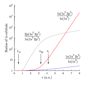
Figure 1: Ratios of the $1s$ and $2p$ orbitals for different configurations of Be. Vertical arrows show rms radii of $1s$ and $2p_{1/2}$ orbitals and the positron turning point $r_{t}$.

As a first example we considered Be atom in different configurations and compared asymptotics of the $1s$ orbital. We used relativistic Hartree-Fock-Dirac code Bratsev et al. (1977) for three closed shell configurations: $1s^{2}$, $1s^{2}2s^{2}$, and $1s^{2}2p_{1/2}^{2}$. Fig. 1 shows the ratio of the $1s$ orbitals for all three cases. One can see that for the configurations $1s^{2}$ and $1s^{2}2s^{2}$ the long distance behaviour is similar. The small difference is caused by a 20% change in the $1s$ energy. We conclude that here numerical results agree with Eq. (2). The $1s$ energy for the configuration $1s^{2}2p_{1/2}^{2}$ lies between the values for two other configurations, but the asymptotics is absolutely different in agreement with Eq. (1). This is in consent with the statement that Eq. (1) applies for the systems with occupied shells with $l\neq 0$ Handy et al. (1969). Fig. 1 also shows the ratio of the $2p_{1/2}$ and $1s$ orbitals for the configuration $1s^{2}2p_{1/2}^{2}$. We see that this ratio first grows exponentially, but then stabilizes at $r\gtrsim 3$ in agreement with (16).

Figure 1 shows that exchange interaction start to determine behaviour of the $1s$ wave function at the distances $r\lesssim r_{2p}$, i.e. near the main maximum of the $2p$ orbital. At such intermediate distances, which lie far behind the classical turning point for the inner electron but in the localization domain of the outer electrons, the exchange interaction is suppressed only by a power of the radius Flambaum (2009a, c).

For the Be atom in $1s^{2}2p_{1/2}^{2}$ configuration the estimate (26) gives $r_{t}\approx 4.2$. Thus, the distances where annihilation can take place are $r\sim 4$. At such distances the difference between $1s$ orbitals with and without exchange interaction (configurations $1s^{2}$ and $1s^{2}2p_{1/2}^{2}$ respectively) is about one order of magnitude. Therefore, the exchange assisted tunneling can enhance annihilation rate (which is proportional to the probability density) by approximately two orders of magnitude. As we see from Fig. 1 the ratio of the $2p$ and $1s$ orbitals at these distances is on the order of $10^{2}$. Therefore, for the Be atom in the configuration $1s^{2}2p^{2}$ we can expect the $1s$ contribution to the annihilation rate to be on the order of $10^{-4}$, instead of $10^{-6}$ without exchange assisted tunneling.

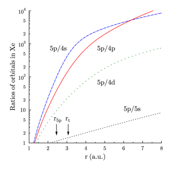
Figure 2: Ratios of the $5p_{3/2}$, $5s_{1/2}$, $4d_{5/2}$, $4p_{3/2}$, and $4s_{1/2}$ orbitals in Xe atom. Vertical arrows show rms radius of $5p_{3/2}$ orbital and the positron turning point $r_{t}$.

Let us consider now a more realistic example. The inner shell contributions to the annihilation $\gamma$ line was studied by Iwata et al. (1997) for several noble gases. For Xe the total probability of the annihilation on the inner shells $4d$, $4p$, and $4s$ was found to be 2.4%. On Fig. 2 we plot the ratios of the orbitals for Xe at the distances from 1 to 8 Bohr radii, where these orbitals do not oscillate. For Xe the estimate (26) for the classical turning point gives $r_{t}\approx 3.1$. At such distances the ratio of the $5p$ and $4d$ orbitals is close to 10. Taking into account that $d$ shell has 10 electrons while $p$ shell has only 6, we conclude that 2% contribution of the $4d$ shell agrees with our simple consideration. The rms radius for the $4d$ orbital in Xe is 0.95 a.u., so such a large contribution is due to the asymptotics (16).

Correlations play very important role in the process of the positron annihilation. They lead to the huge enhancement of the cross section. The electron core polarization leads to the attractive potential for the positron (24) increasing the annihilation rate. Usually this effect has the size of a typical correlation correction for many electron atoms. The dominant correlation corrections come from the positron-electron correlations Dzuba et al. (1993). This type of correlations can lead to the virtual formation of the positronium and neutralization of the positron charge. As a result, the positron can penetrate deeper inside the atom. As we saw above, the classical turning point for the positron $r_{t}$ lies in the region where the electron density of the atom is exponentially decreasing, so even small correlation corrections to $r_{t}$ can drastically increase the annihilation rate. However, it was shown, by Green and Gribakin (2012) that these correlations equally affect outer and inner shell contributions and only slightly change the annihilation line shape. Note that this result indirectly confirms that the densities of the inner and outer electron in the annihilation region are almost proportional to each other, as suggested by Eq. (16).

In this section we considered direct annihilation on the inner shell electron. We argued that this process is enhanced by the exchange interaction between inner and outer shells. The inner shell hole can be also formed in the annihilation on the outer shell followed by ionization of the inner shell caused by the changed atomic potential. In the lowest order of MBPT this process is described by the Coulomb interaction between the inner and the outer shell holes. This Coulomb integral is the same as the exchange integral considered above with substitution of the one final orbital by the orbital in the continuum. Such processes were considered by Dunlop and Gribakin (2006).

Conclusions

In this paper we argue that the exchange assisted tunneling of the electrons from the inner atomic shells is not an artifact of the Hartree-Fock approximation, but an observable effect, at least for the intermediate distances $r\gtrsim 1$. In particular, it can be observed in the annihilation of the slow positrons on the many electron atoms. The annihilation on the inner shell electrons forms the shoulders of the experimentally observed $\gamma$ lines for the noble gases Iwata et al. (1997). It can be also directly detected in the coincidence experiments where $\gamma$ quanta are registered simultaneously with the Auger electrons Eshed et al. (2002). This process takes place at the distances, comparable to the size of the outermost atomic shell. Because of that it is much less suppressed than the inner shell dc field ionization, which may be difficult to observe. On the other hand, without the exchange assisted tunneling of the inner electrons to this region, the inner shell annihilation would be unobservably small. At present we do not see any realistic experiment to test the inner electron asymptotics at the large distances $r\gg 1$ in atomic physics. However such asymptotics can be important in the condensed matter physics Flambaum (2009a).

Appendix A Double well potential

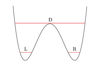
Figure 3: Double well potential with two localized and one delocalized states.

Let us consider a double well potential. We assume that there are two localized states L and R and one delocalized state D with energies $\varepsilon_{L}$, $\varepsilon_{R}$, and $\varepsilon_{D}$ (see Fig. 3). If $\varepsilon_{L}=\varepsilon_{R}=\varepsilon_{LR}$, then the true eigenstates are $\psi_{\pm}=(\psi_{L}\pm\psi_{R})/\sqrt{2}$ and there is exponentially small energy splitting between them:

$$\varepsilon_{\pm}=\varepsilon_{LR}\mp\delta\,, \delta\sim\langle\psi_{L}|\psi_{R}\rangle\,.$$ (27)

The one-particle spectrum of this system is $\varepsilon_{+}$, $\varepsilon_{-}$, and $\varepsilon_{D}$.

If we have two non-interacting electrons in this potential in a triplet state, the spectrum still includes three levels:

$$E_{a}=2\varepsilon_{LR}\,, E_{b,c}=\varepsilon_{LR}+\varepsilon_{D}\mp\delta\,.$$ (28)

If we switch on interaction $1/|x_{1}-x_{2}|$ between the electrons, we get additional splitting between levels $E_{b}$ and $E_{c}$ from the exchange integral:

$$E_{c}-E_{b}=2(\delta+\Delta)\,,$$ (29)

$$\Delta=\left\langle\psi_{L}(x_{1})\psi_{D}(x_{2})\left|\tfrac{1}{|x_{1}-x_{2}|}\right|\psi_{D}(x_{1})\psi_{R}(x_{2})\right\rangle$$

$$\quad\approx-\frac{2}{x_{LR}^{3}}\langle\psi_{L}|x|\psi_{D}\rangle\langle\psi_{D}|x|\psi_{R}\rangle\,.$$ (30)

Here we left the first non-zero term of the multipolar expansion ($x_{LR}$ is the distance between the minima of the potential).

We see that for the non-interacting electrons the splitting is caused by the tunneling through the barrier and is of the order of the overlap integral $\langle\psi_{L}|\psi_{R}\rangle$, which exponentially depends on the distance $x_{LR}$. The exchange interaction with the delocalized electron results in the splitting which depends on this distance as $x_{LR}^{-3}$. The dipole matrix elements in (30) are not suppressed because the state D has large overlaps with both localizes states. We conclude that the exchange interaction can lead to the long range interaction between localized states.

Appendix B $Z^{-1}$ expansion for the He-like ion

The system (10) can be used to form the $\tfrac{1}{Z}$ expansion of the eigenfunction of the highly charged ion. Let us consider He-like ion with $Z\gg 1$. Making substitution $\xi_{i}=Zr_{i}$ we write Hamiltonian (5) as:

$$H^{(2)}\equiv Z^{2}H^{(2)}_{\xi}\\ =Z^{2}\left(-\frac{1}{2}\Delta_{\xi_{1}}-\frac{1}{\xi_{1}}-\frac{1}{2}\Delta_{\xi_{2}}-\frac{1}{\xi_{2}}+\frac{1}{Z}\frac{1}{\xi_{12}}\right)\,.$$ (31)

In the new variables we have

$$H^{(2)}_{\xi}\Psi^{(2)}={\cal E}^{(2)}\Psi^{(2)}\,, {\cal E}^{(2)}\equiv Z^{-2}{E}^{(2)}\,.$$ (32)

We present the solution in the form (8) and need to solve system (10) where

$$W_{i,k}(1)=\frac{1}{Z}\left\langle\phi_{n_{i},l_{i}}(2)\left|\frac{1}{\xi_{1,2}}\right|\phi_{n_{k},l_{k}}(2)\right\rangle\,.$$ (33)

Here the functions $\phi_{n_{i},l_{i}}$ are hydrogenic. Explicit smallness in (33) and, therefore, in the right hand side of Eq. (10a) allows expansion in $Z^{-1}$.

Let us consider the triplet state $1s2p_{m=0}$. The zero-order orbital functions have the form:

$$\Psi_{0}^{(2)} =\frac{1}{\sqrt{2}}\big{(}\phi_{2p_{0}}(1)\phi_{1s}(2)-\phi_{1s}(1)\phi_{2p_{0}}(2)\big{)}\,,$$ (34)

$$\phi_{1s}(\xi) =\frac{2}{\sqrt{4\pi}}\mathrm{e}^{-\xi}\,,$$ (35)

$$\phi_{2p_{0}}(\xi) =\frac{\cos\theta}{4\sqrt{2\pi}}\xi\,\mathrm{e}^{-\xi/2}\,.$$ (36)

Note that already in the first order in $Z^{-1}$ we have infinite number of channels. However, these channels correspond to the different final states of the ion and can be considered independently. We are interested only in the first order corrections to the orbitals $f_{1}$ and $f_{2}$, which correspond to the ion either in the $1s$, or in the $2p$ state:

$$f_{1} =\phi_{2p_{0}}+f^{(1)}_{2p_{0}}\,,$$ (37)

$$f_{2} =\phi_{1s}+f^{(1)}_{1s}+f^{(1)}_{d_{0}}\,.$$ (38)

Note that angular and parity selection rules allow mixing of $s$- and $d$-waves for the amplitude $f_{2}$. However, we will be interested only in the correction to the $s$-wave $f^{(1)}_{1s}$.

For the orbitals (35) and (36) the functions $W_{i,k}$ can be found analytically using Eq. (33):

$$W_{1,1} =\frac{1}{\sqrt{2}Z\xi}\Big{(}1-\mathrm{e}^{-2\xi}(\xi+1)\Big{)}\,,$$ (39)

$$W_{1,2} =-\frac{2\cos\theta}{243Z\xi^{2}}\Big{(}64-\mathrm{e}^{-3\xi/2}(27\xi^{3}$$

$$\qquad+72\xi^{2}+96\xi+64)\Big{)}\,,$$ (40)

$$\tilde{W}_{2,1} =\frac{2}{729Z\xi^{2}\cos\theta}\Big{(}64-\mathrm{e}^{-3\xi/2}(27\xi^{3}$$

$$\qquad+72\xi^{2}+96\xi+64)\Big{)}\,,$$ (41)

$$W_{2,2} =-\frac{1}{\sqrt{2}Z\xi}\Big{(}1-\frac{1}{24}\mathrm{e}^{-\xi}(\xi^{3}$$

$$\qquad+6\xi^{2}+18\xi+24)\Big{)}\,.$$ (42)

In Eq. (B) we left only the term for which the product $\phi_{2p_{0}}\tilde{W}_{2,1}$ has no angular dependence and, therefore, contributes to the $s$-wave part of the amplitude (38).

The first order corrections $f^{(1)}_{2p_{0}}$ and $f^{(1)}_{1s}$ satisfy equations:

$$\left(-\frac{1}{2}\Delta_{\xi}-\frac{1}{\xi}+\frac{1}{8}\right)f^{(1)}_{2p_{0}}\\ =-\phi_{2p_{0}}W_{1,1}-\phi_{1s}W_{1,2}\,,$$ (43)

$$\left(-\frac{1}{2}\Delta_{\xi}-\frac{1}{\xi}+\frac{1}{2}\right)f^{(1)}_{1s}\\ =-\phi_{2p_{0}}\tilde{W}_{2,1}-\phi_{1s}W_{2,2}\,.$$ (44)

These equations are valid at all distances. We see that the right hand sides of both of them have three different exponents, $-\xi/2$, $-\xi$, and $-5\xi/2$. The long-range asymptotics depends on the weakest exponent $-\xi/2$, which corresponds to the binding energy of the electron $2p$. We conclude that the first term of the $Z^{-1}$ expansion has asymptotics in agreement with the general case discussed above.

References

- Handy et al. (1969) N. C. Handy, M. T. Marron, and H. J. Silverstone, Physical Review 180, 45 (1969).
- Dzuba et al. (1982) V. A. Dzuba, V. V. Flambaum, and P. G. Silvestrov, J. Phys. B 15, L575 (1982).
- Flambaum (2009a) V. V. Flambaum, Phys. Rev. A 79, 042505 (2009a), eprint arXiv:0809.2847.
- Morrell et al. (1975) M. M. Morrell, R. G. Parr, and M. Levy, J. Chem. Phys. 62, 549 (1975).
- Katriel and Davidson (1980) J. Katriel and E. R. Davidson, Proceedings of the National Academy of Science 77, 4403 (1980).
- Flambaum (2009b) V. V. Flambaum, Phys. Rev. A 80, 055401 (2009b), eprint arXiv:0909.1868.
- Ruderman and Kittel (1954) M. A. Ruderman and C. Kittel, Physical Review 96, 99 (1954).
- Kasuya (1956) T. Kasuya, Progress of Theoretical Physics 16, 45 (1956).
- Yosida (1957) K. Yosida, Physical Review 106, 893 (1957).
- Fisher et al. (1998) D. Fisher, Y. Maron, and L. P. Pitaevskii, Phys. Rev. A 58, 2214 (1998).
- Flambaum (2009c) V. V. Flambaum, EPL (Europhysics Letters) 88, 60009 (2009c), eprint arXiv:0910.1155.
- Amusia (2009) M. Y. Amusia, Soviet Journal of Experimental and Theoretical Physics Letters 90, 161 (2009), eprint arXiv:0904.4395.
- Iwata et al. (1997) K. Iwata, G. F. Gribakin, R. G. Greaves, and C. M. Surko, Phys. Rev. Lett. 79, 39 (1997).
- Eshed et al. (2002) A. Eshed, S. Goktepeli, A. R. Koymen, S. Kim, W. C. Chen, D. J. O’Kelly, P. A. Sterne, and A. H. Weiss, Phys. Rev. Lett. 89, 075503 (2002).
- Dunlop and Gribakin (2006) L. J. M. Dunlop and G. F. Gribakin, J. Phys. B 39, 1647 (2006), eprint arXiv:physics/0512175.
- Wang et al. (2010) F. Wang, L. Selvam, G. F. Gribakin, and C. M. Surko, J. Phys. B 43, 165207 (2010).
- Surko et al. (2005) C. M. Surko, G. F. Gribakin, and S. J. Buckman, J. Phys. B 38, 57 (2005).
- Dzuba et al. (1993) V. A. Dzuba, V. V. Flambaum, W. A. King, B. N. Miller, and O. P. Sushkov, Physica Scripta T46, 248 (1993).
- Bratsev et al. (1977) V. F. Bratsev, G. B. Deyneka, and I. I. Tupitsyn, Bull. Acad. Sci. USSR, Phys. Ser. 41, 173 (1977).
- Green and Gribakin (2012) D. G. Green and G. F. Gribakin, Journal of Physics Conference Series 388, 072018 (2012).