Critical behavior of self-assembled rigid rods on two-dimensional lattices: Bethe-Peierls approximation and Monte Carlo simulations

Abstract

The critical behavior of adsorbed monomers that reversibly polymerize into linear chains with restricted orientations relative to the substrate has been studied. In the model considered here, which is known as self-assembled rigid rods (SAARs) model, the surface is represented by a two-dimensional lattice and a continuous orientational transition occurs as a function of temperature and coverage. The phase diagrams were obtained for the square, triangular and honeycomb lattices by means of Monte Carlo simulations and finite-size scaling analysis. The numerical results were compared with Bethe-Peierls analytical predictions about the orientational transition for the square and triangular lattices. The analysis of the phase diagrams, along with the behavior of the critical average rod lengths, showed that the critical properties of the model do not depend on the structure of the lattice at low temperatures (coverage), revealing a one-dimensional behavior in this regime. Finally, the universality class of the SAARs model, which has been subject of controversy, has been revisited.

I INTRODUCTION

Self-assembly has become a topic of increasing interest in recent years. One reason for this interest is that it is central to understanding structure formation in living systems Workum . As a consequence, a significant research effort has been devoted to enhance our understanding of the theoretical basis of the fundamental mechanisms governing self-assembly and the observables required to characterize the interactions driving thermodynamic self-assembly transitions Zhang ; Palma . More related to the present work, several research groups reported on the assembly of particles in linear chains Lu ; Scior ; Ouyang ; Tavares0 ; Sciortino . Despite of the number of contributions to this problem, the knowledge of how this process works is still limited.

It is obvious that a complete analysis of the self-assembly phenomenon is quite a difficult subject because of the complexity of the involved microscopic mechanisms. For this reason, the understanding of simple models with increasing complexity might be a help and a guide to establish a general framework for the study of this kind of systems, and to stimulate the development of more sophisticated models which can be able to reproduce concrete experimental situations.

In this context, an interesting model was introduced by Tavares et al. Tavares . The system in Ref. [Tavares, ] consists of monomers with two attractive (sticky) poles that polymerize reversibly into polydisperse chains and, at the same time, undergo a continuous isotropic-nematic (IN) phase transition. Using an approach in the spirit of the Zwanzig model Zwanzig , the authors studied the IN transition occurring in the system. The obtained results revealed that nematic ordering enhances bonding. In addition, the average rod length was described quantitatively in both phases, while the location of the ordering transition, which was found to be continuous, was predicted semiquantitatively by the theory. Finally, Tavares et al. assumed as working hypothesis that the nature of the IN transition remains unchanged with respect to the case of monodisperse rigid rods on square lattices, where the transition is in the 2D Ising universality class GHOSH ; Matoz ; Matoz1 ; Matoz2 .

From the seminal work by Tavares et al., a series of papers exploring the self-assembled rigid rods (SARRs) model have been published Lopez1 ; Almarza1 ; Lopez4 ; Almarza3 ; Lopez2 ; Erratum ; Almarza2 ; Lopez3 ; Lopez5 . These studies can be separated in two groups: (i) those dealing with the nature and universality of the phase transition occurring in the system Lopez1 ; Almarza1 ; Lopez4 ; Almarza3 ; Lopez2 ; Erratum ; Almarza2 and (ii) those dealing with the temperature-coverage phase diagram of the system Lopez3 ; Lopez5 .

With respect to the first point, the universality class of the model has been a subject of controversy. Thus, the criticality of the SARRs model in the square lattice was investigated in Ref. [Lopez1, ] by means of canonical Monte Carlo (MC) simulation and finite-size scaling (FSS) theory. The existence of a continuous phase transition was confirmed. In addition, the determination of the critical exponents, along with the behavior of the Binder cumulants, revealed that the universality class of the IN transition changes from 2D Ising-type for monodisperse RRs without self-assembly to $q=1$ Potts-type (random percolation) for polydisperse SARRs. Later, a multicanonical MC method based on a Wang-Landau sampling scheme was used by Almarza et al. Almarza1 to reinvestigate the critical behavior of the model studied in Refs. [Tavares, ; Lopez1, ]. Employing the crossing point of the Binder cumulants and the value of the critical exponent of the correlation length ($\nu$), it was observed that the criticality of the SARRs model is in the 2D Ising class, as in models of monodisperse RRs Matoz ; Matoz2 .

The results in Refs. [Lopez1, ; Almarza1, ], along with the recent study in Ref. [Lopez4, ], indicate that the system under study represents an interesting case where the use of different statistical ensembles (canonical or grand canonical) leads to different and well-established universality classes ($q=1$ Potts-type or $q=2$ Potts-type, respectively). A similar scheme was observed for triangular lattices, where canonical MC simulations indicated that the IN transition of SARRs at intermediate density belongs to the q=1 Potts universality class Lopez2 ; Erratum . In contrast with this result, a $q=3$ Potts-type universality was obtained by using grand canonical MC simulations Almarza2 .

Among the studies of the second group, the temperature-coverage phase diagram of SARRs on square lattices was calculated in Ref. [Lopez3, ]. By using MC simulations, mean-field theory, and a renormalization group (RSRG) approach, the critical line which separates regions of isotropic and nematic stability was obtained and characterized. The results showed that the theory presented in Ref. [Tavares, ] overestimates the critical temperature in all range of coverage. Small differences appear between simulation and theoretical results for small values of $\theta$; however, the disagreement turns out to be significantly large for larger $\theta$’s. On the other hand, RSRG reproduces qualitatively the shape of the critical line, but systematically underestimates the critical temperature. The main prediction of RSRG approach is that the critical properties of the whole line are associated to a unique second-order fixed point, confirming the continuous nature of the transition. Concerning the MF results, the theory predicts the existence of a first-order transition line and a tricritical point. This finding is in sharp contrast to that obtained by MC simulations and RSRG approach.

More recently, the main adsorption properties of SARRs on square and triangular lattices have been addressed Lopez5 . The study demonstrated that the adsorption isotherms appear as sensitive quantities to the IN phase transition, allowing to reproduce the temperature-coverage phase diagram of the system for square lattices, and to obtain a first determination of the phase diagram for triangular lattices.

Following the line of Refs. [Lopez1, ; Almarza1, ; Lopez4, ; Almarza3, ; Lopez2, ; Erratum, ; Almarza2, ; Lopez3, ; Lopez5, ], the present paper deals with the two aspects above mentioned. On one hand, the problem of the universality is revisited, clarifying recent results obtained for triangular lattices (with conclusions that can be extrapolated to the honeycomb lattice case). On the other hand, the complete temperature-coverage phase diagrams were obtained for the square, triangular and honeycomb lattices by means of MC simulations and FSS analysis. The critical lines were also calculated for the square and triangular lattices within the Bethe-Peierls (BP) or quasi-chemical approach, as formulated in the Cluster Variational Method. Comparisons with MF and RSRG data indicate that BP represents a qualitative advance in the analytical description of the phase diagram of SARRs.

The rest of the paper is organized as follows. In Sec. II we describe the lattice-gas model. The simulation scheme and computational results are given in Sec. III. In Sec. IV we present the analytical approximations, and compare the MC results with the theoretical calculations. In Sec. V we review previous results on the universality class of the SAARs model in the triangular and honeycomb lattices. Finally, the general conclusions are drawn in Sec. VI.

II LATTICE-GAS MODEL

As in Refs. [Tavares, ; Lopez1, ; Lopez2, ; Erratum, ; Lopez3, ; Lopez4, ; Lopez5, ; Almarza1, ; Almarza2, ; Almarza3, ], a system of self-assembled rods with a discrete number of orientations in two dimensions is considered. The substrate is represented by a square, triangular or honeycomb lattice of $M=L\times L$ adsorption sites, with periodic boundary conditions. $N$ particles are adsorbed on the substrate with $m$ possible orientations along the principal axes of the array, being $m=2$ for square lattices and $m=3$ for triangular and honeycomb lattices. The rods interact with nearest-neighbors (NN) through anisotropic attractive interactions. Thus, a cluster or uninterrupted sequence of bonded particles is a self-assembled rod. Then, in the canonical ensemble the adsorbed phase is characterized by the Hamiltonian

$$H=-w\sum_{\langle i,j\rangle}\Big{\{}|\vec{r}_{ij}\cdot\vec{\sigma}_{i}||\vec{r}_{ji}\cdot\vec{\sigma}_{j}|\ {\rm div}\ 1\Big{\}},$$ (1)

where $\langle i,j\rangle$ indicates a sum over NN sites; $w$ represents the NN lateral interaction between two neighboring sites $i$ and $j$; the energy is lowered by an amount $|w|$ only if the NN monomers are aligned with each other and with the intermolecular vector $\vec{r}_{ij}$; $\vec{\sigma}_{j}$ is the occupation vector, with $\vec{\sigma}_{j}=0$ if the site $j$ is empty and $\vec{\sigma}_{j}=\hat{x}_{k}$ if the site $j$ is occupied by a particle with orientation parallel to $x_{k}$. $\hat{x}_{k}$ are a set of unit vectors along the crystalline axes. In Eq.(1) , div represents an integer division, so the result inside { } can be either 0 or 1 (i.e. the fractional part is discarded). The integer division is redundant in the case of the Hamiltonian for the square lattice, but it avoids additional lateral interactions foot0 that promote the condensation of the monomers in the triangular and honeycomb lattice Erratum , restricting the attractive couplings only to those pairs of NN monomers whose orientations are aligned with each other and with the monomer-monomer lattice direction, in line with the model in the square lattice.

The grand canonical Hamiltonian of the model is given by

$$H=-w\sum_{\langle i,j\rangle}\Big{\{}|\vec{r}_{ij}\cdot\vec{\sigma}_{i}||\vec{r}_{ji}\cdot\vec{\sigma}_{j}|\ {\rm div}\ 1\Big{\}}-\left(\mu-\epsilon_{o}\right)\sum_{i}|\vec{\sigma}_{i}|,$$ (2)

where $\epsilon_{o}$ is the adsorption energy of an adparticle on a site and $\mu$ is the chemical potential. In the present work, $\epsilon_{o}=0$ and $\mu$ is the only parameter that determine the strength of the adsorption.

On the other hand, it is worth mentioning that, while the concept of linear rod is trivial for square and triangular lattices, in a honeycomb lattice the geometry does not allow for the existence of a linear array of monomers. In this case, we call linear rod to a chain of adjacent monomers that can be assembled in only three types of sequences, defining three directions in similar way to the triangular lattice. For more details about the model in the honeycomb lattice, see Ref. [Lopez2, ].

In the case of a square lattice the grand canonical Hamiltonian (2) can be exactly mapped into a spin-1 model Lopez3

$$H = -\frac{w}{4}\sum_{<i,j>}\left[(S_{i}^{2}+S_{i})(S_{j}^{2}+S_{j})(\hat{x}_{2}.\vec{r}_{ij})+\right.$$ (3)

$$\left.+(S_{i}^{2}-S_{i})(S_{j}^{2}-S_{j})(\hat{x}_{1}.\vec{r}_{ij})\right]-\mu\sum_{i}S_{i}^{2}$$

where $S_{i}=0,\pm 1$ and $\hat{x}_{1},\hat{x}_{2}$ are unit vectors along the two orthogonal crystalline directions. $S_{i}\pm 1$ represent the vertical ($\vec{\sigma}_{i}=\hat{x}_{2}$) and the horizontal ($\vec{\sigma}_{i}=\hat{x}_{1}$) orientations, while $S_{i}=0$ represents the empty state.

In the case of a triangular lattice the model can be formulated in terms of a diluted $q=3$ anisotropic Potts model. We associate to each site of the lattice a spin variable $\sigma_{i}=0,1,2,3$, such that $\sigma_{i}=0$ represents the empty state and the states $\sigma_{i}=1,2,3$ represent a bar oriented along the three unit vectors $\hat{x}_{k}$ ($k=1,2,3$), where the angle between any pair of them is $2\pi/3$ . Then the Hamiltonian can be written as

$$H = -w\sum_{<i,j>}\sum_{\sigma=1}^{3}\delta(\sigma_{i},\sigma)\,\delta(\sigma_{j},\sigma)\,\delta(\vec{r}_{ij},\pm\hat{x}_{\sigma})-$$ (4)

$$-\mu\sum_{i}\left[1-\delta(\sigma_{i},0)\right]$$

where $\delta(\sigma,\sigma^{\prime})$ is the Kronecker delta function. These alternative representations of the model are useful for the analytical treatment.

III MC SIMULATIONS

III.1 MC method

We have used a standard importance sampling MC method in the canonical and grand canonical ensembles BINDER and FSS techniques PRIVMAN . All calculations were carried out using the parallel cluster BACO of Universidad Nacional de San Luis, Argentina.

III.1.1 Canonical MC simulations

MC simulations in the canonical ensemble were used to obtain the results presented in the subsection III.B. The procedure is as follows. Starting with a random initial configuration (sites occupied with concentration $\theta=N/M$ and particle axis orientation chosen at random), successive configurations are generated by attempting to move single particles (monomers). One of the two (translation or rotation) moves is chosen at random. In a translation move, an occupied site and an empty site are randomly selected and their coordinates are established. Then, an attempt is made to interchange its occupancy state with probability given by the Metropolis rule Metropolis : $P=\min\left\{1,\exp\left(-\beta\Delta H\right)\right\}$, where $\Delta H$ is the difference between the Hamiltonians of the final and initial states and $\beta=1/k_{B}T$ (being $k_{B}$ the Boltzmann constant). For a rotation move, the rotational state of the chosen particle is changed with a probability determined by Metropolis rule. A MC step (MCS) is achieved when $\theta\times M$ sites have been tested to change its occupancy state. Typically, the equilibrium state can be well reproduced after discarding the first $5\times 10^{6}$ MCS. Then, the next $6\times 10^{8}$ MCS are used to compute averages.

III.1.2 Grand canonical MC simulations

MC simulations in the grand canonical ensemble have been carried out to understand the discrepancy between the results of Lopez2 and Almarza2 about the universality class of SAARs model in the triangular lattice (Sec. V). The procedure is as follows. For a given pair of values of $T$ and $\mu$, an initial configuration with $N$ monomers adsorbed at random positions and orientations (on $M$ sites) is generated. Then an adsorption-desorption process is started, where the lattice sites are tested to change its occupancy state with probability given by the Metropolis rule Metropolis : $P=\min\left\{1,\exp\left(-\beta\Delta H\right)\right\}$, where $\Delta H$ is the difference between the Hamiltonians of the final and initial states and $\beta=1/k_{B}T$. Insertion and removal of monomers, with a given orientation, are attempted with equal probability. For this purpose, an axis orientation (with probability $1/3$ for the triangular lattice) and a lattice site are chosen at random. If the selected lattice site is empty, an attempt to place a monomer (with the orientation previously chosen) on the site is made. If, instead, the site is occupied, then the algorithm checks the orientational state of the adsorbed monomer and if this coincides with the previously chosen orientation, an attempt to desorb the particle is performed; otherwise, the trial ends. A MCS is achieved when $M$ sites have been tested to change its occupancy state. The equilibrium state can be well reproduced after discarding the first $6\times 10^{8}$ MCS. Then, averages are taken over $6\times 10^{8}$ successive configurations.

III.1.3 Order parameters, Binder cumulant and FSS analysis

In order to follow the formation of the nematic phase from the isotropic phase, we use the order parameter defined in Ref. Lopez1 for the square lattice,

$$Q=\frac{\left|N_{v}-N_{h}\right|}{N_{v}+N_{h}},$$ (5)

where $N_{h}(N_{v})$ is the number of monomers aligned along the horizontal (vertical) direction, and $N$ is the number of total monomers on the lattice ($N=N_{h}+N_{v}$).

For the triangular and honeycomb lattices, the order parameter has been defined in Ref. [Lopez2, ] as:

$$Q=\frac{\left|\vec{n}_{1}+\vec{n}_{2}+\vec{n}_{3}\right|}{\left|\vec{n}_{1}\right|+\left|\vec{n}_{2}\right|+\left|\vec{n}_{3}\right|},$$ (6)

where each vector $\vec{n}_{i}$ is associated to one of the $3$ possible orientations (or directions) for a chain on the lattice. In addition: $1)$ the $\vec{n}_{i}$’s lie in the same plane (or are co-planar) and point radially outward from a given point $P$ which is defined as coordinate origin; $2)$ the angle between two consecutive vectors, $\vec{n}_{i}$ and $\vec{n}_{i+1}$, is equal to $2\pi/3$; and $3)$ the magnitude of $\vec{n}_{i}$ is equal to the number of rods aligned along the $i$-direction (for a graphical representation, see Fig. 1(a) in Ref. [Lopez2, ]). Note that the $\vec{n}_{i}$’s have the same directions as the $q$ vectors in Ref. [WU, ].

In our canonical MC simulations, we fixed the density $\theta$, and monitored the order parameter $\langle Q\rangle$ as function of temperature $T$. The reduced fourth-order (Binder) cumulant $U_{L}$ BINDER , was calculated as:

$$U_{L}(T)=1-\frac{\langle Q^{4}\rangle}{3\langle Q^{2}\rangle^{2}},$$ (7)

where the thermal average $\langle...\rangle$ means the usual time average throughout the MC simulation.

The critical behavior of the SAARs model has been investigated by means of FSS analysis. The FSS theory implies the following behavior for $\langle Q\rangle$ and $U_{L}$ at criticality:

$$\langle Q\rangle=L^{-\beta/\nu}\tilde{Q}(L^{1/\nu}\epsilon),$$ (8)

and

$$U_{L}=\tilde{U}_{L}(L^{1/\nu}\epsilon),$$ (9)

for $L\rightarrow\infty$, $\epsilon\rightarrow 0$ such that $L^{1/\nu}\epsilon$= finite, where $\epsilon\equiv T/T_{c}-1$ for canonical MC simulations and $\epsilon\equiv\mu/\mu_{c}-1$ for grand canonical MC simulations. Here $\beta$ and $\nu$ are the standard critical exponents of the order parameter ($\langle Q\rangle\sim(-\epsilon)^{\beta}$ for $\epsilon\rightarrow 0^{-}$, $L\rightarrow\infty$), and correlation length $\xi$ ($\xi\sim|\epsilon|^{-\nu}$ for $\epsilon\rightarrow 0,L\rightarrow\infty$), respectively. $\tilde{Q}$ and $\tilde{U}_{L}$ are scaling functions for the respective quantities.

Finally, we calculated the average rod length on the transition line that, at fixed coverage, increases as the temperature decreases. At each MCS the average rod length may be calculated as

$$\overline{\ell}_{MCS}=\frac{N}{N-\left[N_{bonds}-N_{(L)rods}\right]},$$ (10)

where $N$ is the number of monomers adsorbed on the lattice; $N_{bonds}$ is the number of bonds between pairs of nearest-neighbors monomers. $N_{(L)rods}$ is the number of rods with length $L$; its inclusion prevents counting spurious bonds introduced by the periodic boundary conditions (i.e., bonds that do not contribute to the rod’s length). Thus the equilibrium average rod length is obtained from

$$\overline{\ell}={\langle\overline{\ell}_{MCS}\rangle},$$ (11)

III.2 Computational results

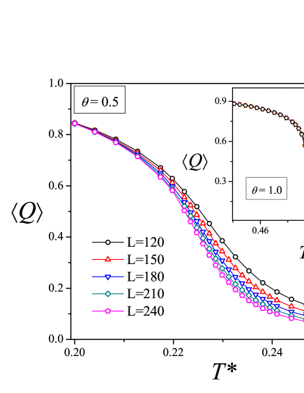
Figure 1: Size dependence of the order parameter as a function of temperature for $\theta=0.5$ and $\theta=1$ (inset).

III.2.1 Behavior of the Binder cumulant

The critical behavior of the SAARs model has been investigated by means of the computational scheme described in the previous section for the canonical ensemble and FSS analysis BINDER ; PRIVMAN . In order to illustrate the behavior of the Binder cumulant in the critical regime, we show here the results for the triangular lattice case at intermediate and full coverage. In addition, these results will be useful when we address the question of whether or not the universality class can change as a result of the constant density constraint applied in the canonical ensemble (Sec. V).

Figure 1 (inset of Fig. 1) shows the behavior of the order parameter versus the reduced temperature $T^{*}=k_{B}T/w$ for several lattice sizes and $\theta=0.5$ foot1 ($\theta=1$). As it can be observed, $\langle Q\rangle$ appears as a proper order parameter to elucidate the phase transition. When the system is disordered ($T^{*}>T^{*}_{c}$, being $T^{*}_{c}$ the critical temperature), all orientations are equivalent and $\langle Q\rangle$ is zero. In the critical regime ($T^{*}<T^{*}_{c}$), the particles align along one direction and $\langle Q\rangle$ is different from zero.

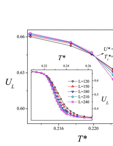
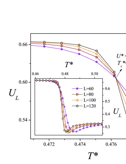
(a) (b)

Figure 2: Curves of $U_{L}$ vs $T^{*}$ for $\theta=0.5$ (a) and $\theta=1$ (b). From their intersections one obtained $T^{*}_{c}$. In the insets, the data are plotted over a wider range of temperatures.

Hereafter we discuss the behavior of the critical temperature as a function of coverage. The standard theory of FSS allows for various efficient routes to estimate $T^{*}_{c}$ from MC data BINDER ; PRIVMAN . One of these methods, which will be used in this case, is from the temperature dependence of $U_{L}(T^{*})$, which is independent of the system size at $T^{*}=T^{*}_{c}$. In other words, $T^{*}_{c}$ can be found from the intersection of the curve $U_{L}(T^{*})$ for different values of $L$, since $U^{*}\equiv U_{L}(T^{*}_{c})=$const. As an example, Fig. 2 shows the reduced four-order cumulants $U_{L}$ plotted versus $T^{*}$ for the cases studied in Fig. 1. The values obtained for the critical temperature were $T^{*}_{c}=0.220(2)$ (corresponding to $\theta=0.5$) and $T^{*}_{c}=0.476(3)$ (corresponding to $\theta=1$).

The behavior of the reduced fourth-order cumulant as a function of temperature also allows to make a preliminary identification of the order and universality class of the phase transition occurring in the system BINDER . Thus, the curves in Fig. 2 exhibit the typical behavior of the cumulants in the presence of a continuous phase transition. Namely, the order parameter cumulant shows a smooth drop from $2/3$ to $0$, instead of a characteristic deep (negative) minimum, as in a first-order phase transition BINDER .

The value of the intersection point $U^{*}$ shows two different behaviors, which can be visualized from Fig. 2. On one hand, the value obtained for $U^{*}$ at $\theta=0.5$ ($U^{*}=0.643(4)$) is consistent with the $q=1$ Potts universality class WU observed in Ref. [Lopez2, ], where the system was studied at a fixed temperature ($T^{*}\approx 0.222$). On the other hand, at $\theta=1$, the fixed value of the cumulants, $U^{*}=0.605(6)$, is more consistent with previous estimates for the three-state Potts model (see for instance Ref. [TOME, ], where $U^{*}\cong 0.613$ foot2 ). However, even though the value of $U^{*}$ may be taken as a first indication of universality, a detailed calculation of critical exponents is required for an accurate determination of the universality class. In Sec. V, the distinction between the two universality classes above is considered based on the determination of the critical exponent of the correlation length.

III.2.2 Phase diagrams of SAARs on square, triangular and honeycomb lattices

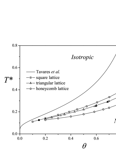
Figure 3: Temperature-coverage diagrams for the SARRs model on different lattices. For comparative purposes, the critical curve reported by Tavares et al. Tavares is shown as a solid line. The open and solid squares are from Refs. [Lopez3, ] and [Almarza1, ], respectively. The open triangles and hexagons represent the results obtained in this work for the triangular and honeycomb lattices, respectively. Solid triangles are from Almarza et al. Almarza2 (in black) and from Ref. [Lopez5, ] (in grey).

The isotropic-nematic phase transition in a model of self-assembled rigid rods with restricted orientations was considered for the first time by Tavares et al. Tavares . The temperature-coverage phase diagram in Ref. [Tavares, ], obtained using an approach in the spirit of the Zwanzig model Zwanzig , is qualitative only, and the theory overestimates the critical temperature in all ranges of coverage (especially at high coverages) foot3 . However, for small values of $\theta$, small differences appear between simulation and theoretical results (Fig. 3). As seen in Fig. 3, the critical lines separate regions of isotropic and nematic stability, and show that the nematic phase is stable at low temperatures and high densities. In addition, the phase diagrams show a marked increase of the density difference from dilute isotropic to dense nematic phases upon increasing the attraction between monomer units (i.e., decreasing the temperature).

The critical line for SARRs on the square lattice, was obtained by means of numerical simulations in Refs. [Lopez3, ] and [Almarza1, ]. Fig. 3 shows the critical line reported in Lopez3 and only one point (the lowest coverage obtained) of the critical line reported in Almarza1 . As explained in Ref. [Almarza1, ], the line of critical points continues beyond the lowest density showed in Fig. 3, however, the rapid increase of the average length of the rods at low densities and temperatures prevents an efficient simulation of the system.

For the case of the triangular lattice, some critical points were obtained, at high coverages in Ref. [Almarza2, ] and at intermediate coverages in Ref. [Lopez5, ] (see Fig. 3). In the latter case, the points were obtained from the singularities in the adsorption isotherms. To corroborate these previous results and complete the phase diagram construction, the procedure used in III.B.1 (to obtain the critical temperature) was repeated for $\theta$ ranging between $0.2$ and $1$. The same procedure was done for the case of the honeycomb lattice, this way the complete phase diagram of honeycomb lattice is reported here for the first time. All results are collected in Fig. 3. Together, the phase diagrams show that the critical properties coincide in the very low-temperature (coverage) regime.

III.2.3 Critical average rod lengths

Using a generalization of the theory of associating fluids, Tavares et al. Tavares obtained an analytic expression for the equilibrium average rod length in the SARRs model, with orientation $\alpha$ along the $x_{1},x_{2}$ directions in two dimensions (2D). In Fig. 4 (inset), we present a comparison between theoretical Tavares and numerical results for the equilibrium average rod length on the transition line. In the numerical case, the points were obtained by using the Eqs. (10) and (11) and square lattices. By comparing these curves it can be seen a qualitative agreement up to $\theta\approx 0.8$. However, at higher coverages, MC simulations show a gradual increase of the critical average rod length, to a value of $\overline{\ell}\approx 7$ (at $\theta=1$). This value is interesting because it coincides with the minimum value of $k$ ($k_{min}=7$), which allows the formation of a nematic phase in long straight rigid rods of length $k$ ($k$-mers and monodisperse case), on a square or triangular lattice GHOSH ; Matoz ; Matoz1 .

The average rod length on the critical line was also obtained for triangular and honeycomb lattices, see Fig. 4. Two observations can be made from Fig. 4: (i) At intermediate coverage ($\theta\approx 0.5$, dashed line), the critical average rod lengths for the square and triangular lattices are similar and near to $7$ (the minimum value of $k$ which allows the formation of a nematic phase in monodisperse rigid rods, on a square or triangular lattice GHOSH ; Matoz ; Matoz1 ). On the other hand, the critical average rod length (at $\theta\approx 0.5$) for the honeycomb lattice, is near to $11$, which coincides with the minimum value of $k$ for the existence of a nematic phase in the case of monodisperse rigid rods on the honeycomb lattice Matoz2 . (ii) Although the trend is more clear for the square and triangular lattices, all lines tend to converge as the coverage decreases towards zero; revealing a one-dimensional behavior in the very low-temperature (coverage) regime. As was shown in Ref. [Almarza2, ], at zero density limit, where the average rod length diverges, an equilibrium polymerization transition occurs.

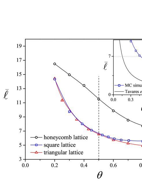
Figure 4: Critical average rod lengths. See description in the text.

IV ANALYTICAL APPROXIMATIONS

In this section we calculate the phase diagram within the Bethe-Peierls (BP) or quasichemical approximation. To do that we use the Cluster Variation Method (CVM) [Tanaka, ]. In the CVM the BP approximation is obtained minimizing a variational free energy expressed in terms of reduced probability densities, namely

$$F = {\rm Tr}\rho H+k_{B}T\left\{(1-q_{c})\sum_{i}{\rm Tr}_{i}\rho_{i}^{(1)}\log\rho_{i}^{(1)}+\right.$$ (12)

$$\left.+\sum_{<i,j>}{\rm Tr}_{i,j}\rho_{i,j}^{(2)}\log\rho_{i,j}^{(2)}\right\},$$

where $q_{c}$ is the coordination number of the lattice, $\rho_{i}^{(1)}$ and $\rho_{i,j}^{(2)}$ are one and two sites reduced densities respectively and it is assumed that $\rho=\prod_{<i,j>}\rho_{i,j}^{(2)}$. $\rho_{i}^{(1)}$ and $\rho_{i,j}^{(2)}$ can be expressed in terms of local one and two site averages, which are used as variational parameters and are related through the reducibility conditions:

$${\rm Tr}_{i}\rho_{i,j}^{(2)} = \rho_{j}^{(1)},$$

$${\rm Tr}_{j}\rho_{i,j}^{(2)} = \rho_{i}^{(1)},$$ (13)

and ${\rm Tr}_{i}\rho_{i}^{(1)}=1$. For details on the method see, e.g. Ref. [Tanaka, ]. In the next subsections we apply the formalism for the models (3) and (4).

IV.1 BP approximation for the square lattice case

Within the representation of the model given by Hamiltonian (3) the orientational order parameter $\langle Q\rangle$ is basically given by the average ”magnetization”

$$m=\frac{1}{M}\left\langle\sum_{i}S_{i}\right\rangle,$$ (14)

while the coverage is given by

$$\theta=\frac{1}{M}\sum_{i}\left<S_{i}^{2}\right>.$$ (15)

Then, the one site probability densities can be expressed as (see Supplementary Material):

$$\rho_{i}^{(1)}(S_{i})=(1-\theta)+\frac{1}{2}\,mS_{i}+(\frac{3}{2}\,\theta-1)S_{i}^{2},$$ (16)

where we have assumed translational invariance. Defining the two-site correlations

$$x_{ij} \equiv \left<S_{i}S_{j}\right>={\rm Tr}_{i,j}S_{i}S_{j}\rho_{i,j}^{(2)},$$ (17)

$$y_{ij} \equiv \left<S_{i}^{2}S_{j}^{2}\right>={\rm Tr}_{i,j}S_{i}^{2}S_{j}^{2}\rho_{i,j}^{(2)},$$ (18)

$$z_{ij} \equiv \left<S_{i}S_{j}^{2}\right>={\rm Tr}_{i,j}S_{i}S_{j}^{2}\rho_{i,j}^{(2)},$$ (19)

$$t_{ij} \equiv \left<S_{j}S_{i}^{2}\right>={\rm Tr}_{i,j}S_{j}S_{i}^{2}\rho_{i,j}^{(2)},$$ (20)

and imposing the reducibility conditions (13), the two site density functions $\rho_{i,j}^{(2)}$ can be obtained in terms of the variational parameters $m$, $\theta$, $x_{ij}$, $y_{ij}$, $z_{ij}$ and $t_{ij}$ (see Supplementary Material). Replacing into Eq.(12) we obtain an expression for the variational free energy, whose derivatives can be handled by means of symbolic manipulation programs. Although solving of the corresponding saddle point equations is cumbersome (even numerically), they greatly simplify in the high temperature case, i.e., when we consider the disordered solution $m=t_{ij}=z_{ij}=0$ which is isotropic: $x_{ij}=x$ and $y_{ij}=y$. In that case we obtain (see Supplementary Material):

$$\log(1+y-2\theta)=2\log(\theta-y)-\log(y-x),$$ (21)

$$x=y\,{\rm tanh}\left(\frac{\beta w}{4}\right),$$ (22)

$$\beta\mu = -\log(2)-2\log(1+y-2\theta)+$$ (23)

$$+3\log\left(\frac{1-\theta}{\theta}\right)+2\,\log(y-x),$$

Working out Eqs.(21)-(23) shows that there is only one physically meaningful solution. The equilibrium coverage $\theta^{*}$ is then given by the solution of the implicit equation

$$e^{-\beta\mu}=F_{-}(\theta^{*},a),$$ (24)

where

$$F_{-}(\theta,a)=2\left[\frac{1+y_{-}(\theta,a)-2\theta}{y_{-}(\theta,a)\,(1-a)}\right]^{2}\,\left(\frac{\theta}{1-\theta}\right)^{3},$$ (25)

with $a\equiv{\rm tanh}(\beta w/4)$ and

$$y_{-}(\theta,a)=\frac{1}{2a}\left[1-a+2a\theta-\sqrt{(1-a+2a\theta)^{2}-4a\theta^{2}}\right],$$ (26)

while the equilibrium values of the correlations are given by $y^{*}=y_{-}(\theta^{*},a)$ and $x^{*}=a\,y^{*}$.

To compute the high temperature nematic susceptibility we add to the Hamiltonian (3) a small external field $B$ conjugated to $m$. Then, at temperatures above the critical one we can still assume isotropy in the solution (namely, the solution of the saddle point equations that converge to the previous one in the limit $B\to 0$), so that $t_{ij}=z_{ij}=z$ and $m\ll 1$, $z\ll 1$. This leads to saddle point equations which expanded to the lowest order in $B^{\prime}\equiv\beta B$ give (see Supplementary Material)

$$3\,\frac{m}{\theta^{*}}=4\,\frac{m-z}{\theta^{*}-y^{*}}-B^{\prime}+{\cal O}(m^{2},z^{2},mz),$$ (27)

$$\frac{z}{x^{*}+y^{*}}=\frac{m-z}{\theta^{*}-y^{*}}+{\cal O}(m^{2},z^{2},mz).$$ (28)

Then, in the linear response regime $m=\chi B^{\prime}$ and $z=\omega B^{\prime}$. In the limit $B^{\prime}\to 0$, $\chi$ is proportional to the nematic susceptibility. From the above equations we obtain

$$\chi = \frac{\theta^{*}(\theta^{*}+x^{*})}{3x^{*}-\theta^{*}},$$ (29)

$$\omega = \frac{\theta^{*}(x^{*}+y^{*})}{3x^{*}-\theta^{*}}.$$ (30)

The disordered solution becomes unstable whenever $3x^{*}=\theta^{*}$. Replacing this condition into Eqs.(21)-(23) we obtain the critical line:

$$e^{-\beta\mu_{c}}=\frac{27}{4}\;\frac{3a-1}{1-a}$$ (31)

and

$$\theta_{c}=3\frac{1-a}{1+3a},$$ (32)

or equivalently:

$$T^{*}_{c}=\frac{1}{4\,{\rm arctanh}\left(\frac{1}{3}\,\frac{3-\theta}{1+\theta}\right)}.$$ (33)

In Fig. 5 we compare the Bethe-Peierls critical line with those obtained by other techniques. From Eq.(33) we obtain the following asymptotic behavior when $\theta\ll 1$:

$$T^{*}_{c}\sim-\frac{1}{2\,\ln\left(\theta\right)},$$ (34)

which agrees qualitatively with the asymptotic behavior of Tavares et al. calculation $T^{*}_{c}\sim-1/3\ln(\theta)$

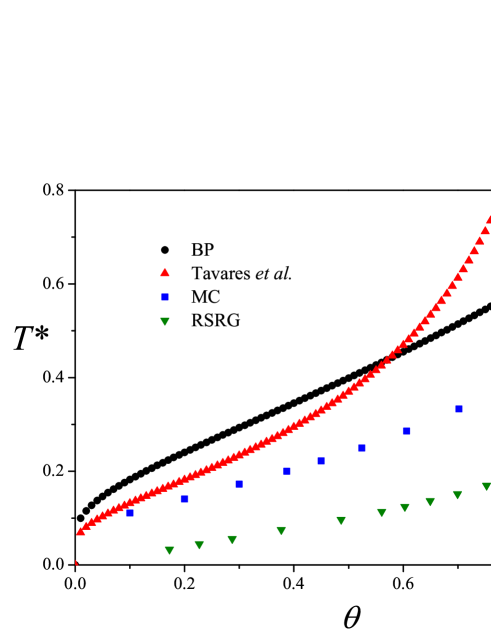
Figure 5: Comparison between the square lattice phase diagram obtained within the Bethe-Peierls (BP) approximation and those obtained by other methods: Real Space Renormalization Group (RSRG) from Ref. [Lopez3, ], Tavares et al. approximation from Ref. [Tavares, ] and MC simulations.

IV.2 BP approximation for the triangular lattice case

The magnetization (orientational order parameter) in this case is given by

$$m = \frac{1}{M}\sum_{i=1}^{M}\left<\left\{\frac{1}{q-1}\left[q\,\delta(\sigma_{i},1)+\delta(\sigma_{i},0)-1\right]\right\}\right>$$ (35)

$$= \frac{1}{2}\left[3\,\left<\delta(\sigma_{i},1)\right>-\theta\right],$$

where the broken symmetry direction $\sigma=1$ is taken arbitrarily among the different $q$ oriented states ($q=3$ in our case). This is a generalization of usual definition for the $q$-state Potts model. In a disordered state we have $\left<\delta(\sigma_{i},1)\right>=\theta/q$, so $m=0$, while in an ordered state along the $\sigma=1$ direction we will have $\left<\delta(\sigma_{i},1)\right>=\theta$ so $m=\theta$. A conjugated external field to the order parameter (35) can be considered by adding to the Hamiltonian (4) a term of the form

$$-\frac{B}{2}\sum_{i}\left[3\,\delta(\sigma_{i},1)+\delta(\sigma_{i},0)-1\right].$$ (36)

The coverage is given by

$$\theta=\frac{1}{M}\sum_{i=1}^{M}\left[1-\left<\delta(\sigma_{i},0)\right>\right]=1-\left<\delta(\sigma_{i},0)\right>.$$ (37)

As in the square lattice case, we will consider hereafter only isotropic solutions (valid above the transition temperature in the $B\ll 1$ limit). We then define the correlations

$$x \equiv \left<\delta(\sigma_{i},0)\,\delta(\sigma_{j},0)\right>,$$ (38)

$$y \equiv \left<\delta(\sigma_{i},1)\,\delta(\sigma_{j},1)\right>,$$ (39)

$$z \equiv \left<\delta(\sigma_{i},2)\,\delta(\sigma_{j},2)\right>=\left<\delta(\sigma_{i},3)\,\delta(\sigma_{j},3)\right>,$$ (40)

$$t \equiv \left<\delta(\sigma_{i},0)\,\delta(\sigma_{j},1)\right>.$$ (41)

The one and two sites reduced densities for the spin variables $\sigma_{i}=0,1,2,3$ can be expressed as

$$\rho_{i}^{(1)}(\sigma_{i})=\sum_{\sigma=0}^{q}P_{\sigma}\delta(\sigma_{i},\sigma)$$ (42)

$$\rho_{i,j}^{(2)}(\sigma_{i},\sigma_{j})=\sum_{\sigma,\sigma^{\prime}}P_{\sigma,\sigma^{\prime}}\delta(\sigma_{i},\sigma)\,\delta(\sigma_{j},\sigma^{\prime}).$$ (43)

Applying the normalization and reducibility conditions the coefficients $P_{\sigma}$ and $P_{\sigma,\sigma^{\prime}}$ can be expressed in terms of the parameters $m,\theta,x,y,z$ and $t$ (see Supplementary Material for details on the calculation).

First of all we checked the mean-field approximation for this model. Inside the CVM formalism, the mean field free energy can be obtained by assuming that the probability density function is given by $\rho=\prod_{i}\rho_{i}^{(1)}$ and keeping up to the first order term in the cummulant expansion of the entropy Tanaka . With a simple analysis (not shown) we found that the mean field approximation predicts a first order transition for any value of $\mu$, in complete disagreement with the numerical simulations.

Replacing the reduced densities into Eq.(12) we obtain the BP free energy in terms of the variational parameters $(m,\theta,x,y,z,t)$ and the corresponding saddle point equations (see Supplementary Material).

At zero field and high enough temperature we have a disordered phase, where all ordered states ($\sigma=1,2,3$) become equally probable and therefore $m=0$ ($\left<\delta(\sigma_{i},1)\right>=\theta/q$). Also from the definitions (39)-(40) we have that $y=z$. With some algebra (see Supplementary Material) the saddle point equations for the disordered solution reduce to

$$\frac{(1-\theta-x)^{6}(1-\theta)^{5}}{x^{6}\theta^{5}}=3e^{\beta\mu},$$ (44)

$$\frac{9zx}{(1-\theta-x)^{2}}=e^{\beta w/3},$$ (45)

$$(1-\theta-x)^{2}=\frac{3}{2}x\,(2\theta+x-1-3z),$$ (46)

$$t=(1-\theta-x)/3.$$ (47)

The physically meaningful solutions of Eqs.(44)-(50) can be obtained in terms of the implicit equation

$$\theta^{*}=G_{-}(\theta^{*}),$$ (48)

where

$$G_{-}(\theta) = \frac{1}{a}\left\{a+x(\theta)(3-a)-\right.$$ (49)

$$\left.-\sqrt{3[ax(\theta)[1-x(\theta)]+3x^{2}(\theta)]}\right\},$$

with $a\equiv 2+e^{\beta w/3}$ and

$$x(\theta)=\frac{(1-\theta)^{11/6}}{3^{1/6}\,e^{\beta\mu/6}\,\theta^{5/6}+(1-\theta)^{5/6}}.$$ (50)

The equilibrium values for the remaining parameters are given by $x^{*}=x(\theta^{*})$, $t^{*}=(1-\theta^{*}-x^{*})/3$ and

$$z^{*}=\frac{e^{\beta w/3}}{9x^{*}}(1-\theta^{*}-x^{*})^{2}.$$ (51)

Equation (48) has always at least two solutions for any value of $\beta$ and $\mu$: $\theta^{*}=1$ ($x^{*}=0$) and $\theta^{*}=0$ ($x^{*}=1$). The first one is the meaningful solution in the limit $\mu\to\infty$. For large but finite values of $\mu$ a third solution with $\theta^{*}<1$ and $1-\theta^{*}\ll 1$ emerges, which decreases with $\mu$. In the $\mu\ll 1$ we obtain the asymptotic behavior (see Supplementary Material)

$$1-\theta^{*}\sim\frac{e^{-\beta\mu}\,3^{5}}{(2+e^{\beta w/3})^{6}},$$ (52)

$$x^{*}\sim\frac{e^{-2\beta\mu}\,3^{9}}{(2+e^{\beta w/3})^{11}},$$ (53)

$$z^{*}\sim\frac{1}{3}\,\frac{e^{\beta w/3}}{2+e^{\beta w/3}}.$$ (54)

Notice that in the $T\to\infty$ ($\beta\to 0$), the correlation $z^{*}\to 1/9$, as expected.

At non zero magnetic field $B\ll 1$ we proceeded as in the square lattice case, by expanding the saddle point equations and keeping the lowest order in $B$. This leads to the following expression for the nematic susceptibility (see Supplementary Material):

$$\chi=\frac{1}{2}\;\frac{\theta^{*}(9z^{*}-x^{*}+1)}{12\theta^{*}-5(9z^{*}-x^{*}+1)},$$ (55)

which diverges when

$$12\theta^{*}-5(9z^{*}-x^{*}+1)=0.$$ (56)

For a given value of the chemical potential $\mu/w$, Eqs.(49) and (58) must be solved together in order to obtain the critical line $T^{*}_{c}$ vs. coverage $\theta$. In Fig.6 we compare a the critical line obtained by numerically solving Eqs.(49) and (58) with the MC results. In particular, in the limit $\mu\to\infty$, when $\theta\to 1$ and $x\to 0$, we obtain from Eqs.(52)-(54) that

$$\chi=\frac{1}{4}\;\frac{3+4\,e^{\beta w/3}}{7-4\,e^{\beta w/3}}.$$ (57)

We see that $\chi>0$ for all temperatures $T>T_{c}$, with

$$T^{*}_{c}=\frac{1}{3\log(7/4)}\approx 0.595647.$$ (58)

and diverges at that temperature, in a clear signature of a second order phase transition. Comparing with the square lattice result from the previous subsection, we see that the critical temperature at $\theta=1$ decreases in the triangular lattice in a factor $\approx 0.826$, which compares well with the MC reduction factor $\approx 0.841$.

For finite, but relatively large values of $\mu/w$, Eqs.(49) and (58) present only one nontrivial solution, that converges to the value given by Eq.(58) in the $\mu\to\infty$ limit. However, for $\mu<\mu_{0}$, with $\mu_{0}\approx-0.65$ (which corresponds to $\theta\approx 0.73$), two new non trivial solutions emerge, one with $\theta\ll 1$ and the other with $1-\theta\ll 1$. As $\mu$ further decreases, the low coverage solution approaches the critical one (i.e., that shown in Fig. 6). Finally, both solutions collapse at $\mu_{c}\approx-0.83$ (corresponding to $\theta\approx 0.24$) and disappear for $\mu<\mu_{c}$. Such behavior could be indicative of the presence of a first order transition at low values of $\mu$, so that the observed secondary instabilities in the susceptibility would correspond to spinodal lines. In that case, a tricritical point somewhere along the calculated transition line should be expected. Indeed, a similar behavior has been observed within the mean field approximation for the square lattice Lopez3 , which disappears in the improved BP approximation as we have shown in the previous subsection. However, to check whether there is a change in the transition order for the triangular lattice case or the observed behavior is just spurious, requires a complete minimization analysis of the BP free energy in a multidimensional space (taking anisotropic ordered solutions into account) which is beyond the scope of the present work. Whatever the case, the calculation presented in Fig. 6 should be regarded as a high coverage approximation.

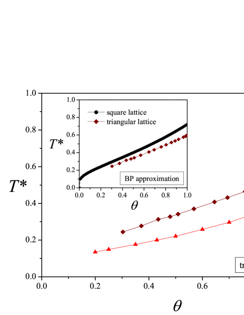
Figure 6: Comparison between the phase diagram obtained within the Bethe-Peierls (BP) approximation and MC simulations for the triangular lattice. Inset: comparison between the BP critical lines for the square and triangular lattices.

V REVISITING THE UNIVERSALITY CLASS

The purpose of this final section is to revisit a number of the issues that have emerged during the course of the discussion about the universality class of the SARRs model, Refs. [Lopez1, ; Almarza1, ; Almarza2, ; Lopez4, ; Almarza3, ]. For the square lattice case foot4 , at intermediate coverages, it was shown that the system under study represents an interesting case where the use of different statistical ensembles (canonical or grand canonical) leads to different and well-established universality classes ($q=1$ Potts type or $q=2$ Potts type, respectively) Lopez4 . In Ref. [Almarza3, ], Almarza et al. concluded that the dependence of the universality class of the SARRs model on the statistical ensemble, is very likely the result of inadequate use of normal scaling to investigate the critical properties of the constrained (constant density) system. However, to date, no completely satisfactory explanation has been given on the consistency of the FSS behavior, in the canonical ensemble, with the critical exponents of the ordinary percolation (i.e. 2D Potts $q=1$ universality class).

As in III.B.1, we will address here only the triangular lattice case. We expect the same universality class for chains on honeycomb lattices (with three allowed orientations), given that the excluded volume term exhibits the same symmetry. The critical behavior of the SAARs model on a triangular lattice was recently reinvestigated by Almarza et al. Almarza2 . The authors found that the isotropic-nematic phase transition occurring in the system is in the 2D Potts $q=3$ universality class. This conclusion contrasts with that of a previous study in the canonical ensemble Lopez2 which indicates that the transition in triangular (and honeycomb) lattices, at intermediate density, belongs to the q = 1 Potts universality class. In Ref. [Almarza2, ], Almarza et al. attributed the discrepancy to the use of the density as the scaling variable in Ref. [Lopez2, ]. In addition, Almarza et al. have cited a paper Fisher in which Fisher showed that fixing the density in some models corresponds to introducing a constraint that renormalizes the critical exponents. More precisely, Almarza et al. have noted that, for the Potts $q=3$ universality class, the renormalized correlation length exponent $\nu^{\prime}$ is $\nu^{\prime}=\nu/(1-\alpha)=5/4$, which is close to the value of $\nu$ for the $q=1$ universality class, $\nu_{q=1}=4/3$, reported in Ref. [Lopez2, ].

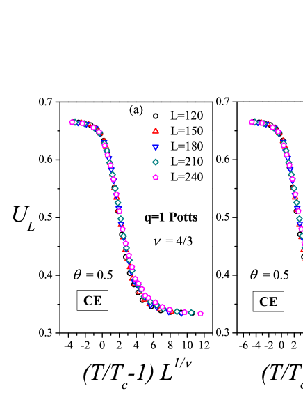
Figure 7: Data collapsing of the Binder cumulant, $U_{L}$ vs $\epsilon L^{1/\nu}$, with the correlation length exponent of the ordinary percolation (a), and with the renormalized exponent (b). CE means canonical ensemble.

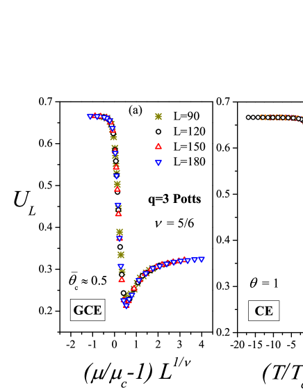
Figure 8: Data collapsing of the Binder cumulant, $U_{L}$ vs $\epsilon L^{1/\nu}$, with the correlation length exponent of the 2D Potts $q=3$ universality class, for: grand canonical ensemble (GCE) simulations at intermediate coverage (a), and canonical ensemble (CE) simulations at full-coverage (b).

In order to test the argument given by Almarza et al., a series of MC simulations have been conducted. As in Refs. [Almarza1, ; Lopez4, ], the distinction between the two universality classes is based on the determination of the value of $\nu$, which is clearly different for the two universality classes under discussion. Then, the scaling behavior can be tested by plotting $U_{L}$ vs $\epsilon L^{1/\nu}$ and looking for data collapse. As shown in Fig. 7(a), the collapse of the curves corresponding to the Fig. 2(a), where the control parameter is the temperature, provides convincing evidence that the scaling obtained using $\nu_{q=1}=4/3$ is not due to the use of the density as the control parameter, as claimed by Almarza et al. However, as would be expected due to the proximity of the values considered here ($\nu_{q=1}$ and $\nu^{\prime}$), a good data collapse with the renormalized correlation length exponent $\nu^{\prime}$ can also be obtained [Fig. 7(b)]. Hence, unlike what happens in the square lattice case, Fisher renormalization arguments appear to be sufficient in the triangular (honeycomb) lattice case.

Moreover, to check the data presented by Almarza et al. Almarza2 , MC simulations in the grand canonical ensemble were carried out using an adsorption-desorption algorithm. It is important to note that the algorithm used here is different from that used by Almarza et al. In the grand canonical ensemble, the critical behavior was studied at the same point of the phase diagram ($\overline{\theta}_{c}\approx 0.5$), fixing the inverse of the reduced temperature to $1/T^{*}=4.5$, and varying the chemical potential $\mu$. Very good collapse was obtained with $\nu=5/6$ in the scaling plot of $U_{L}$ [Fig. 8(a)], thus corroborating the data of Almarza et al. In addition, only in the full-lattice limit ($\theta=1$), canonical MC simulations are able to produce results consistent with the 2D Potts $q=3$ universality class. [see Fig. 8(b), which shows the collapse of the cumulant curves corresponding to the Fig. 2(b)].

Finally, we wish to clarify that: (i) We do not hold that the universality class of the SARRs model depends on the polydispersity of the rods, as was stated by Almarza et al. Almarza3 in reference to our work Lopez4 . (ii) We agree with Almarza et al. that the universality class of the SARRs model, in the square lattice, is that of the 2D Ising model, whereas that in the triangular and honeycomb lattices, is the same as that of the 2D Potts model with $q=3$. (iii) The strong consistency of the results obtained in the canonical ensemble with the critical exponents of the ordinary percolation (at intermediate coverage, in the three lattices considered), warrants an explanation that has not yet been given.

VI CONCLUSIONS

In this paper, the main critical properties of self-assembled rigid rods on square, triangular and honeycomb lattices have been addressed. The results were obtained by using Monte Carlo simulations in the canonical and grand canonical ensembles, finite-size scaling techniques and theoretical analysis in the framework of the Bethe-Peierls approximation.

Several conclusions can be drawn from the present work. On the one hand, the equilibrium average rod length as a function of concentration was calculated by MC simulations. In the case of square lattices, computational data were compared with theoretical results from Tavares et al. Tavares . A good qualitative agreement was observed in the range of coverage from 0 to 0.8. However, the disagreement turns out to be significantly large for $\theta>0.8$. In the case of triangular and honeycomb lattices, the dependence of the equilibrium average rod length on coverage was reported here for the first time.

The obtained results for $\overline{\ell}(\theta)$ reveal two interesting observations: (i) at intermediate coverage ($\theta\approx 0.5$), the value of the average rod length coincides with the minimum value of $k$ ($k_{min}$), which allows the formation of a nematic phase for a system of monodisperse straight rigid $k$-mers adsorbed on two-dimensional lattices (square lattice, $k_{min}=7$ GHOSH ; Matoz ; Matoz1 ; triangular lattice, $k_{min}=7$ Matoz ; Matoz1 and honeycomb lattice, $k_{min}=11$ Matoz2 ); and (ii) at low coverage, the three curves show the same tendency, independently of the lattice geometry (given the range of concentrations studied here, this behavior is more evident for square and triangular lattices). This finding reinforces the idea that the adsorption process behaves as a one-dimensional problem in the low-coverage (temperature) regime: particles adsorb forming chains and an equilibrium polymerization transition occurs in the system Lopez5 .

On the other hand, and regarding the phase diagram of the SARRs, the complete $T$-$\theta$ critical curves corresponding to triangular and honeycomb lattices have been obtained by using MC simulation and FSS analysis. In the case of triangular lattices, the present study allowed us to corroborate previous results obtained from the behavior of the adsorption isotherms Lopez5 and, in the case of honeycomb lattices, the phase diagram has been reported here for the first time.

The simulation phase diagrams were compared with analytical data from the BP approximation. BP results confirm the whole scenario that emerges from the MC simulations, in a clear improvement respect to the mean-field approximation, namely: a) a continuous nature of the phase transition for any value of $\theta$ (although in the triangular lattice case the BP fails in that feature at low coverage, the general trend suggests to be an spurious effect of the approximation); b) a consistent reduction in the critical temperatures for any value $\theta$ when the triangular and square lattice models are compared; c) an independence on $\theta$ of the critical curves for different lattices at very low values of $\theta$ (see inset of Fig.6) and d) a logarithmic decrease with $\theta$ of the critical curve when $\theta\to 0$, in agreement with other analytical approach Tavares .

In an earlier study Lopez3 , in which the critical behavior of SARRs on the square lattice was addressed, it was shown that in the full coverage case ($\theta=1.0$), the Hamiltonian of the SAARs model maps exactly onto the Ising model one ($q=2$ Potts model) with coupling constant $w_{Ising}=w_{SARRs}/4$. In contrast, the 2D SARRs model on the triangular lattice cannot be mapped on $q=3$ Potts model, as can be easily seen from Eq. (4). It is interesting to note, that through a simple extension of the present calculations the critical temperature $T^{*}_{c}$ within the BP approximation for the isotropic $q=3$ Potts model results $3$ times that of the SARRs on the triangular lattice. The corresponding comparison between the critical temperatures extracted from MC simulations predicts a factor $3,3299\approx 10/3$, in close agreement with the BP result.

Finally, the problem of the universality class of the SAARs model was revisited. Since the case corresponding to square lattices has been widely discussed in Refs. [Lopez1, ; Almarza1, ; Lopez4, ; Almarza3, ], we focused in the case of triangular lattices (the same universality class is expected to hold also for honeycomb lattices with three allowed orientations). Based on the calculation of the correlation length exponent $\nu$ in the canonical and grand canonical ensembles, and using the Fisher renormalization scheme, we confirmed previous results by Almarza et al. Almarza2 . Namely, the universality class of the SARRs model for triangular and honeycomb lattices is that of the 2D Potts model with $q=3$. However, the strong consistency of the results obtained in the canonical ensemble with the critical exponents of the ordinary percolation (at intermediate coverage, in the three lattices considered), warrants an explanation that has not yet been given.

- (1) K. Van Workum and J. F. Douglas, Phys. Rev. E 73, 031502 (2006), and references therein.
- (2) Z. Zhang and S. C. Glotzer, Nano Lett. 4, 1407 (2004).
- (3) C-A. Palma, M. Cecchini, and P. Samorì, Chem. Soc. Rev. 41, 3713 (2012).
- (4) X. Lü and J. T. Kindt, J. Chem. Phys. 120, 10328 (2004).
- (5) F. Sciortino, E. Bianchi, J. F. Douglas, and P. Tartaglia, J. Chem. Phys. 126, 194903 (2007).
- (6) W.-Z. Ouyang and R. Hentschke, Phys. Rev. E 79, 031503 (2009).
- (7) J. M. Tavares, L. Rovigatti, and F. Sciortino, J. Chem. Phys. 137, 4901 (2012).
- (8) C. De Michele, T. Bellini, and F. Sciortino, Macromolecules 45, 1090 (2012).
- (9) J. M. Tavares, B. Holder, and M. M. Telo da Gama, Phys. Rev. E 79, 021505 (2009).
- (10) R. Zwanzig, J. Chem. Phys. 39, 1714 (1963).
- (11) A. Ghosh and D. Dhar, EPL 78, 20003 (2007).
- (12) D. A. Matoz-Fernandez, D. H. Linares, and A. J. Ramirez-Pastor, EPL 82, 50007 (2008).
- (13) D. A. Matoz-Fernandez, D. H. Linares, and A. J. Ramirez-Pastor, J. Chem. Phys. 128, 214902 (2008).
- (14) D. A. Matoz-Fernandez, D. H. Linares, and A. J. Ramirez-Pastor, Physica A 387, 6513 (2008).
- (15) L. G. López, D. H. Linares, and A. J. Ramirez-Pastor, Phys. Rev. E 80, 040105(R) (2009).
- (16) N.G. Almarza, J. M. Tavares, and M. M. Telo da Gama, Phys. Rev. E 82, 061117 (2010).
- (17) L.G. López, D.H. Linares, and A.J. Ramirez-Pastor, Phys. Rev. E 85, 053101 (2012).
- (18) N.G. Almarza, J.M. Tavares, and M.M. Telo da Gama, Phys. Rev. E 85, 053102 (2012).
- (19) L.G. López, D.H. Linares, and A.J. Ramirez-Pastor, J. Chem. Phys. 133, 134702 (2010).
- (20) L.G. López, D.H. Linares, and A.J. Ramirez-Pastor, J. Chem. Phys. 134, 079901 (2011).
- (21) N.G. Almarza, J.M. Tavares, and M.M. Telo da Gama, J. Chem. Phys. 134, 071101 (2011).
- (22) L.G. López, D.H. Linares, A.J. Ramirez-Pastor, and S. A. Cannas, J. Chem. Phys. 133, 134706 (2010).
- (23) L.G. López, and A.J. Ramirez-Pastor, Langmuir 28, 14917 (2012).
- (24) If the operation is not used in (1), there will be three possible values of energy between each pair of nearest-neighbor monomers on the triangular (honeycomb) lattice: if they are aligned in the direction of the intermolecular vector ; if one is aligned in the direction of and the other not; and if they are oriented in one direction but different to .
- (25) K. Binder, Applications of the Monte Carlo Method in Statistical Physics. Topics in current Physics, (Springer, Berlin, 1984), Vol. 36.
- (26) V. Privman, Finite Size Scaling and Numerical Simulation of Statistical Systems (World Scientific, Singapore, 1990).
- (27) N. Metropolis, A.W. Rosenbluth, M.N. Rosenbluth, A.H. Teller, and E. Teller, J. Chem. Phys. 21, 1087 (1953).
- (28) In Ref. Lopez2 , we study the critical behavior of the SAARs model on the triangular lattice at and . There, we set the inverse of the reduced temperature to and performed a FSS analysis in terms of density, obtaining . But those results have been recently questioned by Almarza et al. Almarza2 , due to the use of the density as the control parameter. In the present paper, in order to corroborate the previous results, we repeat the scaling treatment, this time maintaining constant the surface coverage (at ) and varying the temperature of the system (the natural control parameter in the canonical ensemble).
- (29) F. Y. Wu, Rev. Mod. Phys. 54, 235 (1982).
- (30) T. Tomé, and A. Petri, J. Phys. A 35, 5379 (2002).
- (31) We have calculated the value of for the standard Potts model in the triangular lattice (with periodic boundary conditions), via MC simulation. The value obtained was , in excellent agreement with those reported in Ref. [TOME, ].
- (32) In Ref. Lopez3 , we have addressed the temperature-coverage phase diagram of self-assembled rigid rods on square lattices by using real space renormalization group (RSRG) approach. The RSRG approach reproduces qualitatively the shape of the critical line, but systematically underestimates the critical temperature.
- (33) T. Tanaka, Methods in Statistical Physics, Cambridge University Press (2002).
- (34) It must be pointed out that the RSRG approach, developed in Ref. Lopez3 for the square lattice, predicts that the whole critical line is in the universality class of the ferromagnetic Ising model, in concordance with the results reported in Ref. Almarza1 .
- (35) M. E. Fisher, Phys. Rev. 176, 257 (1968).