Anderson Impurity in the Bulk of Topological Insulators

Abstract

When an Anderson impurity is immersed in the bulk of a topological insulator that has an ”inverted-Mexican-hat” band-dispersion, a Kondo resonant peak appears simultaneously with an in-gap bound-state. The latter generates another spin state thereby screening the Kondo effect. Using weak-coupling RG scheme, it is shown system exhibits complex crossover behavior between different symmetry configurations and may evolve into a self-screened Kondo or an $SO(n),(n=3,4)$ low energy fixed points. Experimental consequences of these scenarios are pointed out.

I Introduction

The significance of topological insulators (TI) as a new state of matter has been stressed in numerous publications.1 ; 2 ; 3 ; 4 ; 5 ; 6 ; 7 So far, the main attention has been focused on the surface states.8 ; 9 ; 10 ; 11 ; 12 ; 13 ; 14 ; 15 ; 16 ; 17 ; 18 ; 19 ; 20 ; 21 ; 22 ; 22a ; 22b It was pointed out recently that impurity scattering may have non-trivial effects in the bulk of TI due to its peculiar band structure.23 ; 24 ; top-ins-3D-10 ; 3D-TI-QD-12 More concretely, in topological insulators with ”inverted-Mexican-hat” band dispersion around the $\Gamma$-point, in-gap bound states occur due to impurities from which band electrons are scattered (even with arbitrary weak scattering rate).23 In the case of magnetic (Anderson) impurities (forming localized moments) the associated Kondo physics in bulk TI is profoundly distinct from its metallic analog. Using a slave-boson mean-field theory,24 it was shown that an antiferromagnetic exchange interaction $\sim{J}_{df}{\bf{S}}_{d}\cdot{\bf{S}}_{f}$ (with $J_{df}>0$) between the spins of the Anderson impurity $d$ and the induced mid-gap bound-state $f$, leads to a self-screened Kondo effect (KE).24 In fact, the physics described above is not limited to TI but is a general consequence of insulators (and semi-conductors) with a large electronic density of states at the band edge such that in-gap bound states are easily induced by an Anderson impurity.

The goal of this work is to perform a detailed analysis of the interplay between the Anderson impurity and its induced in-gap bound state in bulk TI, and, in particular, elucidate the observable quantities (such as conductivity and magnetic susceptibility) related to the underlying Kondo physics. Employing a weak-coupling renormalization group (RG) analysis, we show that the system exhibits complex crossover behavior between different symmetry sectors and that the exchange interaction $J_{df}$ between the $d$- and $f$-spins may be renormalized dynamically to a negative value at suitable parameters regime. In this case the KE is not screened and the low energy physics of the system is described by an SU(2), SO(4) or SO(3) Kondo fix point. The temperature dependence of the impurity induced resistance and magnetic susceptibility are studied at various regimes.

The article is organized as follows. In Section II, we introduce the model considered starting from a bare Anderson type Hamiltonian. It is shown that the presence of an Anderson impurity $d$ leads to potential scattering of the conduction band electrons, that, in turn, brings about the formation of an in-gap localized quantum state $f$. We introduce the singlet and triplet states of the composite $(d+f)$ impurity. At the end of Section II we arrive at an effective Anderson Hamiltonian that will be analyzed further in the next sections. The local density of states (DOS) is calculated in Section III for the TI with the potential scattering term. Renormalization group analysis is carried out in Section IV. Depending on various energy domains, the RG analysis ends up with various Kondo Hamiltonians that posses different (dynamical) symmetries, SU(2), SO(3) or SO(4). Section V is devoted to the calculations of electric resistivity and magnetic susceptibility in the relevant energy domains. One of the central results of our work is the occurrence of temperature driven crossovers of KE between different symmetry classes. The results are then summarized in Section VI. Some details of the calculation technique are presented in the appendices. These include physical origin of the potential scattering induced by an Anderson impurity (appendix A), discussion of local density of states (appendix B), the SO(4) Kondo Hamiltonian (appendix C), and finally, calculations of electric resistivity (Appendix D) and magnetic susceptibility (Appendix E) for different temperature intervals.

II Model Hamiltonian

Our aim in this section is to derive an effective Hamiltonian that, in addition to the Anderson impurity $d$, contains also the mid-gap state $f$ as discussed in Ref [24, ]. Starting from an Hamiltonian describing an Anderson impurity $d$ in the bulk of a TI, a few manipulations are required to transform it into its workable form, Eq. (18a) below. The bare Hamiltonian is,

$$H=H_{0}+H_{d}+H_{t}^{(0)}+V.$$ (1)

Here the first term, $H_{0}$, describes electrons in the bulk of the TI,

$$H_{0}=\sum_{\bf{k}}\Psi^{\dagger}_{\bf{k}}~{}h_{0}({\bf{k}})~{}\Psi_{\bf{k}},$$

$$h_{0}({\bf k})=\hbar v_{F}\big{(}{\bf{k}}\cdot\bm{\alpha}\big{)}+\beta M_{k},$$ (2)

$$\Psi^{\dagger}_{\bf k}=\Big{(}a^{\dagger}_{{\bf k}\uparrow},a^{\dagger}_{{\bf k}\downarrow},b^{\dagger}_{{\bf k}\uparrow},b^{\dagger}_{{\bf k}\downarrow}\Big{)}.$$

where $M_{k}=mv_{F}^{2}-B\hbar^{2}k^{2}$, $a^{\dagger}_{{\bf k}\sigma}$, $b^{\dagger}_{{\bf k}\sigma}$ are creation operators for electron of momentum ${\bf k}$ and spin projection $\sigma$. $h_{0}({\bf k})$ is written in particle-hole $\otimes$ spin space, with $\bm{\alpha}=t_{x}\otimes{\bf{s}}$ and $\beta=t_{z}\otimes{s_{0}}$, where ${\bf{t}}=(t_{x},t_{y},t_{z})$ or ${\bf{s}}=(s_{x},s_{y},s_{z})$ are vectors of the Pauli matrices acting in the space of isospins or spins, $s_{0}$ is the $2\times 2$ identity matrix. $H_{d}$ is the Hamiltonian for the Anderson impurity,

$$H_{d}=\epsilon_{d}\sum_{\sigma}n_{d\sigma}+U_{d}n_{d\uparrow}n_{d\downarrow},$$ (3)

where $\epsilon_{d}$ is the impurity energy level and $U_{d}$ is the interaction between electrons on the impurity. $n_{d\sigma}=d_{\sigma}^{{\dagger}}d_{\sigma}$, $d_{\sigma}^{{\dagger}}$ or $d_{\sigma}$ is the creation or annihilation operator of electron on the d-level. The hybridization between the Anderson impurity $d$ and the band electrons is described by

$$H_{t}^{(0)}=V_{d}\sum_{{\bf{k}},\sigma}\left(a_{{\bf{k}}\sigma}^{{\dagger}}d_{\sigma}-ib_{{\bf{k}}\sigma}^{{\dagger}}d_{\sigma}+{\text{H.c.}}\right).$$ (4)

The last term appearing in the Hamiltonian (1) is an effective potential scattering between band-electrons induced by the impurity,

$$V=V_{0}\sum_{{\bf{k}},\bf{k}^{\prime}\sigma}\Big{(}a_{{\bf{k}}\sigma}^{{\dagger}}-ib_{{\bf{k}}\sigma}^{{\dagger}}\Big{)}\Big{(}a_{{\bf{k}}^{\prime}\sigma}+ib_{{\bf{k}}^{\prime}\sigma}\Big{)}.$$ (5)

A few words on the origin of the potential scattering term $V$ are in order. When an Anderson impurity is immersed in a metal it leads to an $s-d$ Hamiltonian and to a potential scattering. In the standard analysis of the Anderson impurity, the induced potential scattering term is neglected because it is irrelevant as far as Kondo physics is concerned. The situation is different when the impurity is immersed in an insulator. Here, as we shall see in the following, the potential scattering leads to a mid gap bound-states that profoundly affects the underlying physics. The detailed discussions about the physical origin of the strength $V_{0}$ and the derivation of the localized in-gap $f$-level are given in Appendix A.

Diagonalization of $H_{0}$
The eigenstates of $H_{0}$ alone is given by

$$H_{0} = \sum_{\nu\sigma{\bf{k}}}\nu\varepsilon_{k}\gamma_{\nu{\bf{k}}\sigma}^{{\dagger}}\gamma_{\nu{\bf{k}}\sigma},$$ (6a)

where $$\nu=\pm 1 c/v$$ or denotes the conduction and valence band.

$$\varepsilon_{k}=\sqrt{M_{k}^{2}+(\hbar v_{F}k)^{2}},\ \ \ M_{k}=mv_{F}^{2}-B\hbar^{2}k^{2},$$ (6b)

is the band dispersion. $$\gamma_{\nu{\bf{k}}\sigma}^{{\dagger}} \gamma_{\nu{\bf{k}}\sigma}$$ and are creation and annihilation operators of quasi-particle defined through the transformation,

$$\tilde{\Psi}_{\bf{k}}={\cal{S}}_{k}{\cal{U}}_{k}\Psi_{\bf{k}},\ \ \ \ \ \tilde{\Psi}_{\bf{k}}^{{\dagger}}=\Big{(}\gamma_{c{\bf{k}}\uparrow},\gamma_{c{\bf{k}}\downarrow},\gamma_{v{\bf{k}}\uparrow},\gamma_{v{\bf{k}}\downarrow}\Big{)},$$

$${\cal{U}}_{k}=\cos\frac{\alpha_{k}}{2}+i\sin\frac{\alpha_{k}}{2}~{}t_{y}\otimes({\bf{s}}\cdot{\bf{e}}_{k}),$$ (6c)

where $${\bf{e}}_{k}={\bf{k}}/k$$,

$$\tan\Big{(}\frac{\alpha_{k}}{2}\Big{)}=\sqrt{\frac{\varepsilon_{k}-M_{k}}{\varepsilon_{k}+M_{k}}}.$$

$${\cal{S}}_{k} h_{0}({\bf{k}}) {\cal{U}}_{k}$$ is a unitary matrix which commute with and .

$\varepsilon_{k}$ is gapped and the insulator is topological for $Bm>0$. For $Bm>1/2$ (assumed hereafter), the band dispersion has an ”inverted-Mexican-hat” form (see Figure 1) with dispersion minimum at a surface of nonzero wave-vector $\mathbf{q}$’s, with

$$\varepsilon_{q}=\frac{v_{F}^{2}}{2B}~{}\sqrt{4Bm-1},\ \ \ \ \ q=\frac{v_{F}}{\hbar B}~{}\sqrt{Bm-\frac{1}{2}},$$ (7)

where $q=|\mathbf{q}|$.

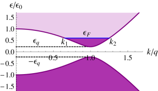
Figure 1: Energy dispersion (6b) for $Bm=20$. The dark (bright) regions denote the energy levels below (above) the Fermi energy $\epsilon_{F}$. The band-edges occur at momentum $q$ at energies $\pm\varepsilon_{q}$. (Here it is assumed that $\varepsilon_{q}<\epsilon_{F}<mv_{F}^{2}$). $k_{1}$ and $k_{2}$ are two solutions of the equation $\varepsilon_{k}=\epsilon_{F}$.

Transformation of $H_{t}^{(0)}$ and $V$
Here we express the terms $H_{t}^{(0)}$ and $V$ defined in equations (4) and (5) in terms of the quasiparticle operators. Applying the unitary transformation (6c) to the tunnel Hamiltonian (4), we get

$$H_{t} = \sum_{\bf{k}}\Bigg{\{}\tilde{\Psi}_{\bf{k}}^{{\dagger}}{\cal{S}}_{k}\bigg{(}\begin{array}[]{c}{\cal{V}}_{k}\\ -i{\cal{V}}_{k}\end{array}\bigg{)}\bigg{(}\begin{array}[]{c}d_{\uparrow}\\ d_{\downarrow}\end{array}\bigg{)}+{\rm{H.c.}}\Bigg{\}},$$

where ${\cal{V}}_{k}$ is a $2\times 2$ unitary matrix,

$${\cal{V}}_{k} = \cos\alpha_{k}-i\sin\alpha_{k}({\bf{s}}\cdot{\bf{e}}_{k}),\ \ \ \ \ {\cal{V}}_{k}^{{\dagger}}{\cal{V}}_{k}=1.$$

Choosing ${\cal{S}}_{k}$ as,

$${\cal{S}}_{k} = \left(\begin{array}[]{cc}{\cal{V}}_{k}^{{\dagger}}&0\\ 0&i{\cal{V}}_{k}^{{\dagger}}\end{array}\right),$$ (11)

we get,

$$H_{t}=V_{d}\sum_{{\bf{k}},\nu,\sigma}\left(\gamma_{\nu{\bf{k}}\sigma}^{{\dagger}}d_{\sigma}+d^{{\dagger}}_{\sigma}\gamma_{\nu{\bf{k}}\sigma}\right).$$ (12)

Applying transformations (6c) and (11) to the potential scattering Hamiltonian (5), we get,

$$V = V_{0}\sum_{\nu\nu^{\prime}{\bf{kk}}^{\prime}\sigma}\gamma_{\nu{\bf{k}}\sigma}^{{\dagger}}\gamma_{\nu^{\prime}{\bf{k}}^{\prime}\sigma}.$$

Diagonalization of $H_{0}+V$: Mid-gap state.
The next step is crucial, as it demonstrates the formation of a mid-gap state $f$ due to the potential scattering term $V$. Because the potential $V$ emerges due to the Anderson impurity, we say that the mid-gap state is induced by the impurity. In order to find the eigenstates of $H_{0}+V$, we solve the Heisenberg equation of motion

$$i\hbar\dot{\gamma}_{\nu{\bf{k}}\sigma}=\big{[}H_{0}+V,\gamma_{\nu{\bf{k}}\sigma}\big{]}.$$

Taking $\gamma_{\nu{\bf{k}}\sigma}(t)=\gamma_{\nu{\bf{k}}\sigma}e^{-i\epsilon t/\hbar}$, we get

$$\epsilon\gamma_{\nu{\bf{k}}\sigma} = \nu\varepsilon_{k}\gamma_{\nu{\bf{k}}\sigma}+V_{0}\sum_{\nu^{\prime}{\bf{k}}^{\prime}}\gamma_{\nu^{\prime}{\bf{k}}^{\prime}\sigma}.$$ (13)

Equation (13) has nontrivial solution when $\epsilon$ satisfies the secular equation,

$$\sum_{\nu{\bf{k}}}\frac{V_{0}}{\epsilon-\nu\varepsilon_{k}} = 1.$$ (14)

The solutions for $|\epsilon|\geq\varepsilon_{q}$ describe the band electrons, whereas the solution for $|\epsilon|<\varepsilon_{q}$ corresponds to the localized $f$-level.

It is seen that when $|\epsilon|<\varepsilon_{q}$, the expression in the left hand side of the secular equation (14) is positive when $\epsilon$ is negative and negative when $\epsilon$ is positive [$V_{0}$ is assumed to be positive here]. When $|\epsilon|\to\varepsilon_{q}$, the sum diverges as $\big{(}\varepsilon_{q}^{2}-\epsilon^{2}\big{)}^{-1/2}~{}{\rm{sign}}(-\epsilon)$ for energy bands with the “inverted Mexican hat” structure.24 As a result, the secular equation gives us a mid-gap energy level $\epsilon_{f}$ which lies within the interval $-\varepsilon_{q}<\epsilon_{f}<0$. When $\epsilon_{f}+\varepsilon_{q}\ll\varepsilon_{q}$, we can write

$$\epsilon_{f}\approx-\varepsilon_{q}~{}\sqrt{1-\Big{(}\frac{V_{0}q}{2\pi\hbar^{2}B}\Big{)}^{2}}.$$ (15)

This procedure leads to a minor modification of the annihilation and creation operators for the band electrons. Strictly speaking they are respectively expressed as linear combination of $\gamma_{\nu{\bf{k}}\sigma}$ and $\gamma_{\nu{\bf{k}}\sigma}^{{\dagger}}$ using perturbation theory with $V_{0}$ as a small parameter. However, since the potential pulls only one level (out of many) from the band into the gap, the other levels are virtually unaffected. In what follows, we assume that the operators for the modified levels inside the band just slightly differs from the $\gamma_{\nu{\bf{k}}\sigma}$ and $\gamma_{\nu{\bf{k}}\sigma}^{{\dagger}}$ . Thus, the main outcome of the potential scattering is the creation of a midgap level $f$. The annihilation operator $f_{\sigma}$ for this localized level is given by,

$$f_{\sigma}=\sum_{\nu{\bf{k}}}\frac{AV_{0}}{\epsilon_{f}-\nu\varepsilon_{k}}~{}\gamma_{\nu{\bf{k}}\sigma},$$ (16)

$$A=\Bigg{(}\sum_{\nu{\bf{k}}}\frac{V_{0}^{2}}{\big{(}\epsilon_{f}-\nu\varepsilon_{q}\big{)}^{2}}\Bigg{)}^{-\frac{1}{2}}.$$

Hybridization term $H_{df}$
The last ingredient in our quest for constructing an effective tunneling Hamiltonian with $d$ and $f$ impurities is to identify a hopping term $H_{df}$ between the Anderson impurity and the mid-gap state. The hybridization term $H_{t}^{(0)}$ between the bulk TI electrons and the $d$-impurity level leads to an effective tunneling term $H_{df}$ between the $d$ impurity and the $f$ in-gap bound state, and an effective tunneling term $H_{t}$ between the $d$ impurity and the band states. We assume that $H_{t}$ is still given by equation (12), whereas $H_{df}$ is

$$H_{df} = V_{df}\sum_{\sigma}\left(f^{{\dagger}}_{\sigma}d_{\sigma}+d^{{\dagger}}_{\sigma}f_{\sigma}\right),$$ (17)

where ${V}_{df}\sim{V}_{d}$.

The effective Hamiltonian
Finally, to arrive at the desired effective tunneling Hamiltonian we collect all pieces into a sum of three parts structured as “band+composite impurity+hybridization” Hamiltonians,

$$H = H_{l}+H_{C}+H_{t}.$$ (18a)

Here $$H_{l}=H_{0}+V$$ is the Hamiltonian of the two band electrons that include also the potential scattering term, and

$$H_{C} = H_{d}+H_{f}+H_{df},$$ (18b)

is the Hamiltonian of the composite impurity, including the $$d f H_{d} H_{df}$$- and -levels. is given by equation (3), is given by equation (17), and

$$H_{f} = \epsilon_{f}\sum_{\sigma}n_{f\sigma}+U_{f}n_{f\uparrow}n_{f\downarrow},$$ (18c)

where $$\epsilon_{f} f U_{f} f n_{f\sigma}=f_{\sigma}^{{\dagger}}f_{\sigma} H_{t}$$ is the single-electron energy (15) of the localized -level, is the interaction between electrons on the -level, and . The hybridization term is given by equation (12).

Energy scales
Few words about energy scales are in order: Unless otherwise specified, we shall assume $U_{d}\rightarrow\infty$ and

$$\epsilon_{F}-D_{0}<\epsilon_{d}\ll\epsilon_{f}<\epsilon_{F}<\epsilon_{f}+U_{f}\ll\epsilon_{F}+D_{0},$$ (19)

where $D_{0}$ (the initial bandwidth) is the highest energy cutoff, and $\epsilon_{F}$ is the Fermi energy (see Figure 1). We use $\epsilon_{F}=2\varepsilon_{q}$, $\epsilon_{f}\approx-\varepsilon_{q}$, $U_{f}=5\varepsilon_{q}$ and $\epsilon_{d}=-80\varepsilon_{q}$ in the following calculations.

The eigenstates of $H_{C}$
Equation (18b) are specified by the configuration numbers $(N_{d},N_{f})$ representing the number of electrons on the levels $d$ and $f$. With energy scales specified by (19) the ground state has $N_{d}=N_{f}=1$ and there are four possible states, a spin-singlet state $|S\rangle$ and three spin-triplet states $|T_{m}\rangle$ ($m=0,\pm 1)$. The singlet energy is modified when $V_{df}\neq 0$ while the triplet energy is unaffected. Explicitly,

$$|S\rangle=\left\{\frac{\alpha_{S}}{\sqrt{2}}\Big{(}d_{\uparrow}^{{\dagger}}f_{\downarrow}^{{\dagger}}-d_{\downarrow}^{{\dagger}}f_{\uparrow}^{{\dagger}}\Big{)}-\beta_{f}f_{\uparrow}^{{\dagger}}f_{\downarrow}^{{\dagger}}\right\}|0\rangle,$$ (20a)

$$\begin{array}[]{l}\displaystyle|T_{1}\rangle=d_{\uparrow}^{{\dagger}}f_{\uparrow}^{{\dagger}}|0\rangle,\ \ \ \ \ |T_{-1}\rangle=d_{\downarrow}^{{\dagger}}f_{\downarrow}^{{\dagger}}|0\rangle,\\ \\ \displaystyle|T_{0}\rangle=\frac{1}{\sqrt{2}}\Big{\{}d_{\uparrow}^{{\dagger}}f_{\downarrow}^{{\dagger}}+d_{\downarrow}^{{\dagger}}f_{\uparrow}^{{\dagger}}\Big{\}}|0\rangle,\end{array}$$ (20e)

where

$$\varepsilon_{S}=\epsilon_{d}+\epsilon_{f}-\frac{2V_{df}^{2}}{\Delta_{f}},\ \ \ \ \ \varepsilon_{T}=\epsilon_{d}+\epsilon_{f},$$

$$\alpha_{S}=\sqrt{1-\beta_{f}^{2}},\ \ \ \ \ \beta_{f}={\sqrt{2}V_{df}\over\Delta_{f}},$$

$$\Delta_{f}=\epsilon_{f}-\epsilon_{d}+U_{f}.$$

In the absence of hybridization of d-electron with the band electrons (i.e., when $V_{d}=0$), $\varepsilon_{S}<\varepsilon_{T}$, and the spin singlet state has lower energy.

III Local density of states

Because of the potential scattering, the local density of states (DOS) depends on the energy $\varepsilon$ of an electron and on the distance $r$ from the impurity,

$$\rho(\varepsilon,r)=-\frac{1}{\pi}~{}{\rm{Im}}\sum_{\nu\nu^{\prime}{\bf{k}}{\bf{k^{\prime}}}}G_{\nu{\bf{k}},\nu^{\prime}{\bf{k}}^{\prime}}(\varepsilon)e^{i({\bf{k}}-{\bf{k}}^{\prime}){\bf{r}}},$$ (21)

$$G_{\nu{\bf{k}},\nu^{\prime}{\bf{k}}^{\prime}}(\varepsilon)=\int\tilde{G}_{\nu{\bf{k}},\nu^{\prime}{\bf{k}}^{\prime}}(t)e^{\frac{(i\varepsilon-\eta)t}{\hbar}}dt.$$ (22)

Here $\eta$ is a positive infinitesimal parameter, $\tilde{G}_{\nu{\bf{k}},\nu^{\prime}{\bf{k}}^{\prime}}(t)$ is a retarded Green’s function,

$$\tilde{G}_{\nu{\bf{k}},\nu^{\prime}{\bf{k}}^{\prime}}(t)=-\frac{i}{\hbar}~{}\Theta(t)~{}\Big{\langle}\Big{\{}\gamma_{\nu{\bf{k}}\sigma}(t),\gamma_{\nu^{\prime}{\bf{k}}^{\prime}\sigma}^{{\dagger}}\Big{\}}\Big{\rangle},$$ (23)

where $\langle\cdots\rangle$ denotes the thermal average with respect to the Hamiltonian $H_{0}+V$.

Applying the Heisenberg equation of motion (13), we get the following expression for the local DOS,

$$\rho(\varepsilon,r) = \rho_{0}(\varepsilon)~{}\frac{1+\pi^{2}V_{0}^{2}~{}\big{[}\rho_{0}^{2}(\varepsilon)-\rho_{0}^{2}(\varepsilon,r)\big{]}}{1+\pi^{2}V_{0}^{2}~{}\rho_{0}^{2}(\varepsilon)},$$ (24)

where

$$\rho_{0}(\varepsilon,r)=\Theta(|\varepsilon|-\varepsilon_{q})~{}\frac{\rho_{c}~{}|\varepsilon|}{2\sqrt{\varepsilon^{2}-\varepsilon_{q}^{2}}}~{}\Bigg{\{}\Theta(\varepsilon_{0}-|\varepsilon|)~{}\frac{\sin\big{(}qrg_{1}(\varepsilon)\big{)}}{qr}+\frac{\sin\big{(}qrg_{2}(\varepsilon)\big{)}}{qr}\Bigg{\}},\ \ \ \ \ \rho_{0}(\varepsilon)=\rho_{0}(\varepsilon,0).$$ (25)

Detailed derivation of the local DOS is given in Appendix B.

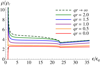
Figure 2: Local DOS (24) for $\varepsilon_{0}=24\varepsilon_{q}$, $V_{0}\rho_{c}=0.06$ and different values of $qr$.

The local DOS (24) is shown in Figure 2 for different values of $qr$. It is seen that $\rho(\epsilon,0)$ vanishes as $\big{(}\epsilon^{2}-\epsilon_{q}^{2}\big{)}^{\frac{1}{2}}$ when $|\epsilon|\to\epsilon_{q}$. When $qr>2$, $\rho(\epsilon,r)$ approaches $\rho_{0}(\epsilon)$, the bare DOS.

IV Renormalization-Group (RG) Analysis

Within RG analysis, high energy charge fluctuations are integrated out and one reaches a low energy spin ($s-d$) Hamiltonian. The latter is written in terms of the spin operator ${\bf s}$ of the band electrons and a collection of vector operators of the composite impurity. These vector operators generate a dynamical symmetry group that characterize the pertinent Kondo physics.28 If the ground state of $H_{C}$ contains a single electron the symmetry group is SU(2), while if the ground state of $H_{C}$ contains two electrons the symmetry group can be SO(3) [see equation (40)] or SO(4) [see equation (35)]. Technically, the high energy degrees of freedom are successively integrated out such that $D_{0}\rightarrow D<D_{0}$ is reduced and energies are renormalized. For the Kondo effect in metals, where the DOS is virtually constant, this is a standard procedure. The fact that $\rho(\varepsilon)\neq$const. requires some modifications. We introduce the following definitions,

$$\bar{\rho}(D)=\frac{1}{2}~{}\Big{[}\rho(\epsilon_{F}+D)+\rho(\epsilon_{F}-D)\Big{]},$$ (26)

$${\cal L}(D_{1},D_{2})=\int\limits_{D_{1}}^{D_{2}}\frac{2~{}\bar{\rho}(D)~{}dD}{\rho_{c}~{}D}.$$ (27)

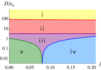
Figure 3: Parametric diagram $j-D$ for $\epsilon_{d}=-80\varepsilon_{q}$, $\varepsilon_{0}=24\varepsilon_{q}$ and $\epsilon_{F}=2\varepsilon_{q}$. The curves separate the different temperature intervals: the red curve is $D_{i}=\epsilon_{F}-\varepsilon_{d}$ separating the regimes (i) [mixed valence regime] and (ii) [SU(2) Kondo regime], the purple line is $D_{ii}$ separating the regimes (ii) [SU(2) Kondo regime] and iii [SO(4) Kondo regime], the blue curve is $D_{iii}=|J_{df}|$ [$J_{df}<0$] separating the regimes (iii) [SO(4) Kondo regime] and (iv) [SO(3) Kondo regime], whereas the green curve is $D_{iii}=|J_{df}|$ [$J_{df}>0$] separating the regimes (iv) [SO(4) Kondo regime] and (v) [self screened Kondo regime].

The RG flow is divided into the following regimes (see Figure 3):

• $\epsilon_{d}>\epsilon_{F}-D>\epsilon_{F}-D_{0}$, in which charge fluctuations in both $d$ and $f$ states exist and there is no KE;

• $\epsilon_{F}-D>\epsilon_{d}$ but $\epsilon_{f}(\sim-\varepsilon_{q})>\epsilon_{F}-D$ or $\epsilon_{F}+D>2\epsilon_{f}+U_{f}$, where charge fluctuations on the $d$ orbital is quenched but still exist on the $f$ orbital. The system is in the single impurity ($SU(2)$) Kondo impurity regime;

• $\epsilon_{F}-D>\epsilon_{f}$ and $\epsilon_{F}+D<2\epsilon_{f}+U_{f}$, but $D>|J_{df}|$ where charge fluctuations in both $d$ and $f$ orbitals are quenched, but the singlet-triplet energy splitting can be neglected. The singlet and triplet states can be considered as degenerate and the system demonstrate the SO(4) Kondo regime.

• The system is at the $SO(3)$ Kondo regime [if $J_{df}<0$, interval (iv)] or the self-screened Kondo regime [if $J_{df}>0$, interval (v)]. These regimes exist only if $U_{f}>\epsilon_{F}-2\epsilon_{f}\sim$ a few $\varepsilon_{q}$.

The RG analysis for the various regimes now follows:

Regime (i): Charge fluctuations on the $d$-orbital are integrated out as in Ref. [Haldane-78, ], but here the spin-singlet and spin-triplet energies are, generically, renormalized distinctly. Renormalization of other quantities such as $V$, $\epsilon_{f}$ and $V_{df}$ are weak and can be ignored. The scaling procedure of $\varepsilon_{S(T)}$ then yields,Hewson-book ; Kikoin-Avishai-02

$$\frac{d\varepsilon_{S(T)}}{d\ln{D}}=V_{S(T)}^{2}~{}\rho(\varepsilon_{F}+D),$$ (28)

where $V_{S}^{2}=\alpha_{S}^{2}V_{d}^{2}$ and $V_{T}^{2}=V_{d}^{2}$. The difference between $V_{S}^{2}$ and $V_{T}^{2}$ originates from the appearance of the normalization factor $\alpha_{S}$ in the singlet state [see (20a)]. Notice that $V_{S}^{2}<V_{T}^{2}$ and the triplet energy level renormalizes faster than the singlet level. This opens the possibility that, as RG stops, the ground state of the system may become a triplet if the single-triplet level crossing occurs before quenching of charge fluctuations in the $d$- and $f$-levels. Solving equation (28), we find that the singlet-triplet energy spacing $J_{df}^{(i)}(D)=\varepsilon_{T}(D)-\varepsilon_{S}(D)$ is given by

$$J_{df}^{(i)}(D)\sim\beta_{f}^{2}\Delta_{f}\left(1-\frac{2V_{d}^{2}\rho_{0}}{\Delta_{f}}~{}\frac{\sqrt{D_{0}}-\sqrt{D}}{\sqrt{\varepsilon_{0}}}\right).$$ (29)

where $D=D_{i}\sim\epsilon_{F}-\epsilon_{d}$ at the end of scaling.

Regime (ii): Charge fluctuations of the $d$-level are quenched at $D_{i}\sim\epsilon_{F}-\epsilon_{d}$. A Schrieffer-Wolf transformation for the d-level, yields an effective Hamiltonian

$$H^{(ii)}_{I}=H_{0}+H_{f}+H_{df}+H_{K}^{(ii)},$$

where

$$H_{K}^{(ii)}={1\over 2}\sum_{\alpha_{\sigma},\beta_{\sigma}=\gamma_{\sigma},f_{\sigma}}J_{\alpha\beta}\left(\alpha^{\dagger}_{\sigma}{{\mathbf{s}}_{\sigma\sigma^{\prime}}}\beta_{\sigma^{\prime}}\right)\cdot\mathbf{S}_{d},$$ (30)

where

$$\gamma_{\sigma}=\sum_{\nu,\mathbf{k}}\gamma_{\nu\mathbf{k}\sigma},$$

${\mathbf{s}}$ is the vector of Pauli matrices, $\mathbf{S}_{d}$ is the localized spin of the $d$-level and

$$J_{\gamma\gamma}=\frac{2V_{d}^{2}}{\epsilon_{F}-\epsilon_{d}},\ \ \ \ \ J_{ff}=\frac{2V_{df}^{2}}{\epsilon_{f}-\epsilon_{d}},$$

$$J_{\gamma f}=J_{f\gamma}=\frac{V_{d}V_{f}}{\epsilon_{f}-\epsilon_{d}}+\frac{V_{d}V_{f}}{\epsilon_{F}-\epsilon_{d}}.$$

The Hamiltonian $H_{K}^{(ii)}$ describes coupling of the $d$-spin to $\gamma$ and $f$ electrons. Notice that charge fluctuations in the $f$-orbital is allowed in $H_{K}^{(ii)}$ through the mixed spin operators

$$\mathbf{S}_{m}=\frac{1}{2}~{}\left(\gamma^{{\dagger}}_{\sigma}{\mathbf{s}_{\sigma\sigma^{\prime}}}f_{\sigma^{\prime}}\right)$$

and $\mathbf{S}_{m}^{{\dagger}}$. Figure 4 clarifies the physics of the various interactions encoded in $H_{K}^{(ii)}$.

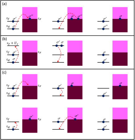
Figure 4: Transitions induced by $H_{K}^{(ii)}$, equation (30) leading from an initial state on the left and ending at a final state on the right. The various processes are associated with exchange constants (a): $J_{\gamma\gamma}$, (b): $J_{ff}$ and (c): $J_{\gamma f}$ and $J_{f\gamma}$

.

Using poor-man scaling,Anderson-70 charge fluctuations in the $f$-orbital can now be integrated out. The dimensionless exchange coupling constants $j_{\alpha\beta}\equiv\rho_{0}J_{\alpha\beta}$ are renormalized as,

$$\frac{dj_{\alpha\beta}}{d\ln{D}}=-j_{\alpha\gamma}j_{\gamma\beta}~{}\frac{\bar{\rho}}{\rho_{0}},$$ (31)

with the solution (see equation (26) for ${\cal L}(D,D_{i})$),

$$j_{\alpha\beta}(D)=j_{\alpha\beta}(D_{i})+\frac{j_{\alpha\gamma}(D_{i})j_{\gamma\beta}(D_{i}){\cal{L}}(D,D_{i})}{\displaystyle 1-j_{\gamma\gamma}(D_{i}){\cal{L}}(D,D_{i})}.$$ (32)

The scaling invariant, that is, the Kondo temperature $T_{K}^{(ii)}$, is got by solving the equation

$$j_{\gamma\gamma}(D_{i}){\cal{L}}(T_{K}^{(ii)},D_{i})=1,$$ (33)

and scaling stops if

$$T_{K}^{(ii)}>D_{ii}=\min\big{\{}\epsilon_{F}-\epsilon_{f},U_{f}-\epsilon_{F}+\epsilon_{f}\big{\}},$$

at which the $d$-spin is quenched by the KE. This happens if $j_{\gamma\gamma}(D_{i})$ is large enough. We note that ${\cal{L}}(D_{ii},D_{i})$ remains finite as long as $D_{ii}>T_{K}^{(ii)}$. For $T_{K}^{(ii)}<D_{ii}$, scaling stops at $D=D_{ii}$ and the $d$-spin is not quenched. The effective coupling between $f$- and $d$-spins is a sum of contributions from $H_{df}$ and $H_{K}^{(ii)}$, i.e. $J_{df}=J_{df}^{(i)}(D_{i})+J_{ff}(D_{ii})$. It is ferromagnetic if $J_{df}<0$. Assuming that $1-j_{\gamma\gamma}(D_{i}){\cal{L}}(D_{ii},D_{i})$ is of order $O(1)$, $\epsilon_{F}\sim\varepsilon_{q}<\varepsilon_{0}\ll|\epsilon_{d}|$ and $U_{f}$ is a few $\varepsilon_{q}$ [$\varepsilon_{q}\ll|\epsilon_{d}|$], we find that $J_{ff}(D_{ii})$ is of the same order as $\beta_{f}^{2}\Delta_{f}$ and $J_{df}<0$ if

$$|V_{d}|^{2}\geq\varepsilon_{0}^{3\over 2}~{}\sqrt{|\epsilon_{d}|}.$$

Regimes (iii) and (iv): The scaling stops at regime (ii) with $D_{ii}\sim\epsilon_{F}+\varepsilon_{q}$ if the chemical potential is located inside the band-gap which is the usual case for insulators. A more interesting scenario occurs if the chemical potential $\epsilon_{F}$ is located above the band-gap which may happen if the insulator is doped by impurities. Scaling continues in this case where charge fluctuations in $f$-level is also quenched. In this case the mixed spin term $\mathbf{S}_{m}$ becomes ineffective and we are left with an effective Hamiltonian $H^{(2)}=H_{0}+H_{K}^{(iii)}$, where

$$H_{K}^{(iii)}=J_{K}\mathbf{S}_{\gamma}\cdot\mathbf{S}_{d}+J_{df}\mathbf{S}_{f}\cdot\mathbf{S}_{d},$$ (34)

where

$$\mathbf{S}_{\gamma}={1\over 2}\sum_{\mathbf{k}\sigma,\mathbf{k}^{\prime}\sigma^{\prime},\nu}\left(\gamma^{{\dagger}}_{\nu\mathbf{k}\sigma}{\mathbf{s}}_{\sigma\sigma^{\prime}}\gamma_{\nu\mathbf{k}^{\prime}\sigma^{\prime}}\right),$$

and

$$J_{K}=J_{\gamma\gamma}(D_{ii})=\frac{J_{\gamma\gamma}(D_{i})}{1-j_{\gamma\gamma}(D_{i}){\cal{L}}(D_{ii},D_{i})}.$$

Notice that $|J_{df}|$ is in general smaller than $J_{K}$.24

$SO(3)$ and $SO(4)$ fixed points: For $D_{ii}\gg|J_{df}|$, there exists a regime $D\gg|J_{df}|$ where the system is governed by a critical point between the $SO(3)$- and the quenched-Kondo regimes which has $SO(4)$ symmetry.27 In this regime the behavior of the system is governed by the $SO(4)$ critical point. The system crossovers to the low temperature $SO(3)$- or self-screened-Kondo regime at $D<|J_{df}|$. We first consider the $SO(4)$ regime $D\gg|J_{df}|$.

SO(4) Kondo fixed point: In this case we may set $J_{df}=0$ and apply the Schrieffer-Wolf transformation directly to the spin-singlet and triplet states to get,

$$H_{K}^{SO(4)} = J_{T}\big{(}{\bf{S}}\cdot{\bf{S}_{\gamma}}\big{)}+J_{ST}\big{(}{\bf{R}}\cdot{\bf{S}_{\gamma}}\big{)},$$ (35)

where ${\bf{S}}$ and ${\bf{R}}$ are the ($S=1)$ spin and the Runge-Lenz operators, respectively that are expressible in terms of Hubbard operators for the composed impurity, and satisfy the $so(4)$ algebra.28 The exchange constants $J_{T}=J_{K}/2$ and $J_{ST}=\alpha_{S}J_{T}$ scale as,

$$\frac{dj_{T}}{d\ln{D}} = -\big{(}j_{T}^{2}+j_{ST}^{2}\big{)}~{}\frac{{\bar{\rho}}}{\rho_{0}},$$ (36a)

$$\frac{dj_{ST}}{d\ln{D}} = -2j_{T}j_{ST}~{}\frac{{\bar{\rho}}}{\rho_{0}}.$$ (36b)

The combinations $j_{n}=j_{T}-(-1)^{n}j_{ST}$ [$n=1,2$] satisfy,

$$j_{n}(D) = \frac{j_{n}(D_{ii})}{\displaystyle 1-j_{n}(D_{ii})~{}{\cal{L}}(D,D_{ii})},$$ (37)

whence

$$j_{T}(D)~{}=~{}\frac{1}{2}~{}\Big{[}j_{1}(D)+j_{2}(D)\Big{]},$$ (38a)

$$j_{ST}(D)=~{}\frac{1}{2}~{}\Big{[}j_{1}(D)-j_{2}(D)\Big{]}.$$ (38b)

The corresponding Kondo temperature $T_{K_{4}}$ is determined from the equation,

$$\Big{\{}j_{T}(\bar{D}_{ii})+j_{ST}(\bar{D}_{ii})\Big{\}}~{}{\cal{L}}(T_{K_{4}},\bar{D}_{ii}) = 1$$ (39)

provided $T_{K_{4}}\gg|J_{df}|$. For $0<T_{K_{4}}<J_{df}$ the two spins form a spin-singlet (self-screened KE) at $D\sim J_{df}$.

SO(3) Kondo fixed point: For $J_{df}<0$ and $T_{K_{4}}<|J_{df}|$, renormalization of $j_{ST}$ stops at $D=D_{iii}\sim|J_{df}|$. For $D<D_{iii}$, the Kondo Hamiltonian becomes

$$H_{K}^{SO(3)} = J_{T}{\bf{S}}\cdot{\bf{S}_{\gamma}}.$$ (40)

The scaling equation for $j_{T}=J_{T}\rho_{0}$ and its solution are,

$$\frac{dj_{T}}{d\ln{D}}=-j_{T}^{2}~{}\frac{{\bar{\rho}}}{\rho_{0}},$$ (41a)

$$j_{T}(D)=\frac{j_{T}(D_{iii})}{\displaystyle 1-j_{T}(D_{iii}){\cal{L}}\big{(}D,D_{iii}\big{)}}.$$ (41b)

Scaling stops at $T_{K_{3}}$ determined from the equation,

$$j_{T}\big{(}D_{iii}\big{)}~{}{\cal{L}}\big{(}T_{K_{3}},D_{iii}\big{)} = 1.$$ (42)

V Resistivity and Impurity Magnetic Susceptibility

Having elaborated upon the theory in the weak coupling regime $T\gg T_{K}$’s we are now in a position to carry out perturbation calculations of experimental observables. In 3D, the most accessible ones are the impurity resistivity $R_{\rm{imp}}(T)$ and the impurity magnetic susceptibility $\chi_{\rm{imp}}(T)$. We shall be guided by the quest to find out how the special features of the TI’s are reflected in these observables. These features are the occurrence of gap and the structure of the DOS especially near the band edges $\pm\varepsilon_{q}$. In addition, reducing the temperature results in the crossover between different scaling regimes of the couplings. Explicitly, there are three relevant temperature regimes denoted as (ii),(iii),(iv) in order to match the notation of the corresponding scaling regimes discussed previously. The first regime, denoted as (ii), is defined by [$D_{i}>T>D_{ii}$] as given by equation (31) for the scaling interval (ii). Local moment behavior exists only at the $d$-level in this regime and therefore there is Kondo scattering with SU(2) symmetry. The second regime, denoted as (iii), is defined by equation (36) for scaling interval (iii) [$D_{ii}>T>D_{iii}$]. Here one may neglect the difference in energies between the singlet and triplet states and the system is at the $SO(4)$ Kondo regime. The third regime, denoted as (iv), is defined by equation (41a) for scaling interval (iv) [$D_{iii}>T>T_{K_{3}}$]. Here there is Kondo scattering with $SO(3)$ symmetry (when $J_{df}<0$) or a self-screened KE if $J_{df}>0$. The temperature dependence of the resistivity and magnetic susceptibility in these three different scaling regimes are distinct.

In the calculation of resistivity, we assume $\epsilon_{F}>\varepsilon_{q}$ (the TI is doped) and the system has a Fermi surface. The impurity resistivity as calculated in the framework of the “poor man’s scaling” formalism is given by,

$$R_{\rm{imp}} = \frac{N_{\nu}R_{0}}{{\cal{L}}^{2}(T_{K_{\nu}},T)},$$ (43)

where $\nu=(ii),(iii),(iv)$, denotes the pertinent temperature regime as detailed above. The corresponding Kondo temperatures are $T_{K_{ii}}$, equation (33), $T_{K_{iii}}\equiv{T}_{K_{4}}$, equation (39), or $T_{K_{iv}}\equiv{T}_{K_{3}}$, equation (42). The numerical factors $N_{\nu}$ are, $N_{ii}=N_{iii}=3/4$ and $N_{iv}=2$. Here

$$R_{0}=\frac{3\pi c_{\rm{imp}}}{\hbar e^{2}\rho_{0}^{2}}~{}\frac{1}{v_{1}^{2}+v_{2}^{2}},\ \ \ \ \ v_{i}\approx\frac{1}{\hbar}~{}\bigg{(}\frac{\partial\varepsilon_{k_{i}}}{\partial k_{i}}\bigg{)},$$

and $k_{1},~{}k_{2}$ are two solutions of $\varepsilon_{k}=\epsilon_{F}$ (see Figure 1).

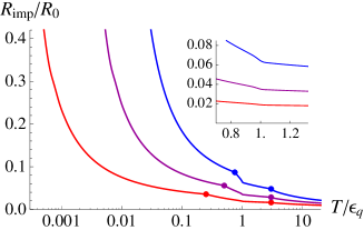
Figure 5: Resistivity (43) as a function of temperature for $\epsilon_{d}=-80\varepsilon_{q}$, $\varepsilon_{0}=24\varepsilon_{q}$, $\epsilon_{F}=2\varepsilon_{q}$ and different values of $j$: $j=0.1$ [bottom red curve], $j=0.12$ [middle purple curve] and $j=0.14$ [top blue curve]. The dots denote $T=D_{ii}$ and $T=D_{iii}$ separating the temperature intervals (ii), (iii) and (iv). Inset: behavior of $R_{\rm{imp}}$ for the temperature $T\sim\varepsilon_{q}$.

The resistivity as a function of the temperature is shown in Fig.5 assuming a low temperature $SO(3)$ fix point. It is seen that $R_{\rm{imp}}$ has different temperature dependence within the temperature intervals (ii), (iii) and (iv), with crossover observed at $T=D_{ii}$ and $T=D_{iii}$ [the points $D_{ii}$ and $D_{iii}$ are denoted by dots]. In addition, crossovers are observed at $T=\varepsilon_{q}$ [interval (iii)]. These crossovers appear since the function ${\cal{L}}(T_{K_{iii}},T)$ changes its behavior at $T=\epsilon_{F}-\varepsilon_{q}=\varepsilon_{q}$ [we take $\epsilon_{F}=2\varepsilon_{q}$ here].

The Kondo scattering manifests itself also in the magnetic susceptibility.Hewson-book The impurity susceptibility calculated in the framework of the “poor man’s scaling” is

$$\chi_{\rm{imp}} = \frac{K_{\nu}\chi_{0}T_{K_{ii}}}{T}~{}\bigg{\{}P_{\nu}-\frac{1}{{\cal{L}}(T_{K_{\nu}},T)}\bigg{\}},$$ (44)

where $\nu=(ii),(iii),(iv)$, the Kondo temperatures are $T_{K_{ii}}$, equation (33), $T_{K_{iii}}\equiv{T}_{K_{4}}$, equation (39), and $T_{K_{iv}}\equiv{T}_{K_{3}}$, equation (42). The numerical factors are $K_{ii}=K_{iii}=1/4$, $K_{iv}=2/3$, $P_{ii}=P_{iv}=1$ and $P_{iii}=2$. The constant $\chi_{0}$ is

$$\chi_{0}=\frac{4c_{\rm{imp}}\mu_{B}^{2}}{T_{K_{ii}}}.$$

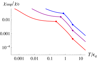
Figure 6: Magnetic susceptibility (44) as a function of temperature for $\epsilon_{d}=-80\varepsilon_{q}$, $\varepsilon_{0}=24\varepsilon_{q}$, $\epsilon_{F}=2\varepsilon_{q}$ and different values of $j$: $j=0.1$ [red curve], $j=0.12$ [purple curve] and $j=0.14$ [blue curve]. The dots denote $T=D_{ii}$ and $T=D_{iii}$ separating the temperature intervals (ii), (iii) and (iv).

The impurity magnetic susceptibility as a function of $T$ is shown in Figure 6. The different temperature dependences of $\chi_{\rm{imp}}$ at different temperature regimes (ii), (iii) and (iv) are obvious, with crossovers observed at $T=D_{ii}$ and $T=D_{iii}$ [the points $D_{ii}$ and $D_{iii}$ are denoted by dots].

VI Conclusions

We have analyzed the interplay between the Anderson impurity and its induced in-gap bound state in a model of 2D topological insulator. Using a weak-coupling RG analysis, it is shown that the exchange interaction $J_{df}$ between the $d$- and the induced in-gap $f$-spins may be renormalized dynamically to either positive or negative values. The parameters required to observe the above phenomena is not too restrictive ($|V_{d}|^{2}\geq\varepsilon_{0}^{3\over 2}\sqrt{|\epsilon_{d}|}$, $\varepsilon_{q}<U_{f}\ll{U}_{d}$) and is realistic. The system exhibits complex crossover behaviors at different parameter regimes as a result which can be observed in the temperature dependence of the impurity induced resistance and magnetic susceptibility. The crossover in the temperature dependence of both the resistivity and the impurity magnetic susceptibility at different regimes is a peculiar feature that can serve as an experimental confirmation of the above analysis. For both screened and under-screened Kondo effect in the weak coupling regime, the effective coupling constant $j$ renormalizes as $1/{\cal{L}}(T_{K},T)$ (or, as $1/\ln(T/T_{K})$, when the DOS is flat, see Ref. [Hewson-book, ]). As a result, the impurity resistivity, $R_{\rm{imp}}$, behaves as $1/{\cal{L}}^{2}(T_{K},T)$ [see equation (43)], whereas the susceptibility, $\chi_{\rm{imp}}$, is given by equation (44).

The physics described above is not limited to TI but is a general consequence of (doped) insulators (and semi-conductors) with a large electronic density of states at the band edge such that in-gap bound states are easily induced by an Anderson impurity. Similar physics may be found in for example, two-layer graphene systems. Our paper is just a first step towards understanding the rich physics associated with impurities in these systems.

Acknowledgements: Discussions with C. M. Varma are highly appreciated. We acknowledge support by HKRGC through grant HKUST03/CRF09. The research of I.K and Y.A is partially supported by grant 400/12 of the Israeli Science Foundation (ISF).

Appendix A Interpretation of $V_{0}$ in equation (5)

Electrons in an lattice move in the periodic potential $w_{l}({\bf{r}})$,

$$w_{l}({\bf{r}}) = \sum_{\bf{n}}w_{a}({\bf{r}}-{\bf{n}}),$$ (45)

where $w_{a}({\bf{r}})$ is the interaction energy of electrons with an lattice atom, ${\bf{n}}=n_{1}{\bf{a}}_{1}+n_{2}{\bf{a}}_{2}+n_{3}{\bf{a}}_{3}$, ${\bf{a}}_{1,2,3}$ are the lattice vectors, $n_{1,2,3}$ are integers. In this case, electrons tunnel from one atom to another and the single-electron atomic levels $\epsilon_{a}$ reduce to the energy band shown in Figure 7.

When the atom of the lattice at the point ${\bf{r}}={\bf{0}}$ is replaced by an impurity atom, the potential energy $w_{i}({\bf{r}})$ of interaction of electrons with the impurity differs from $w_{a}({\bf{r}})$. As a result, the potential energy of electrons in the lattice with the impurity,

$$w({\bf{r}}) = \sum_{{\bf{n}}\neq 0}w_{a}({\bf{r}}-{\bf{n}})+w_{i}({\bf{r}}),$$ (46)

is not periodic anymore (see the purple curve in Figure 7).

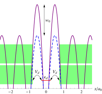
Figure 7: Potential energy of electrons in the lattice with the impurity put at the point ${\bf{r}}={\bf{0}}$. The solid purple curve is the potential energy (46), whereas the dashed blue curve is the potential energy (45) of electrons in the lattice without impurity. The filled areas denote the valence and conduction bands. The red line is the impurity level. It is assumed that $|{\bf{a}}_{1,2,3}|=a_{0}$ and ${V_{d}}\ll{w_{0}}$, where $V_{d}$ is the hybridization rate between $d$-impurity and the band electrons.

Then the potential scattering can be estimated as,

$$V_{0} = \int{d^{3}{\bf{r}}}~{}\Big{\{}w_{i}({\bf{r}})-w_{a}({\bf{r}})\Big{\}}\sim$$ (47)

$$\sim w_{0}~{}a_{0}^{3},\ \ \ \ \ w_{0}=w_{i}^{(0)}-w_{a}^{(0)},$$

where $w_{i}^{(0)}$ or $w_{a}^{(0)}$ is the peak of the potential energy of the impurity or the atom. Here we assume that the electric potential is screened at the inter-atomic distance $a_{0}$.

Appendix B Local Density of States

The potential scattering $V$, equation (5), results in modification of the density of states and formation of an in-gap energy level . In order to derive an explicit expression for the local DOS (21), we calculate the retarded Green’s function (22). Applying the equation of motion (13), we get

$$G_{\nu{\bf{k}},\nu^{\prime}{\bf{k}}^{\prime}}(\varepsilon) = g_{\nu k}(\varepsilon)~{}\delta_{kk^{\prime}}~{}\delta_{\nu\nu^{\prime}}+V_{0}~{}g_{\nu k}(\varepsilon)\sum_{\nu^{\prime\prime}{\bf{k}}^{\prime\prime}}G_{\nu^{\prime\prime}{\bf{k}}^{\prime\prime},\nu^{\prime}{\bf{k}}^{\prime}}(\varepsilon),$$ (48)

where

$$g_{\nu k}(\varepsilon)=\frac{1}{\varepsilon-\nu\varepsilon_{k}+i\eta}.$$

The solution of equation (48) is,

$$G_{\nu{\bf{k}},\nu^{\prime}{\bf{k}}^{\prime}}(\varepsilon) = g_{\nu k}(\varepsilon)~{}\delta_{kk^{\prime}}~{}\delta_{\nu\nu^{\prime}}+$$ (49)

$$+ \frac{V_{0}~{}g_{\nu k}(\varepsilon)~{}g_{\nu^{\prime}k^{\prime}}(\varepsilon)}{\displaystyle 1-V_{0}\sum_{\nu^{\prime\prime}{\bf{k}}^{\prime\prime}}g_{\nu^{\prime\prime}k^{\prime\prime}}(\varepsilon)}.$$

Then the DOS (21) is

$$\rho(\varepsilon,r)=\rho_{0}(\varepsilon)-{\rm{Im}}\frac{\pi V_{0}\big{\{}{\cal{R}}^{2}(\varepsilon,r)+\pi^{2}\rho_{0}^{2}(\varepsilon,r)\big{\}}}{1+\pi V_{0}\big{\{}{\cal{R}}(\varepsilon,0)+i\rho_{0}(\varepsilon,0)\big{\}}},$$ (50)

where ${\cal{R}}(\varepsilon,r)$ and $\rho_{0}(\varepsilon,r)$ are real and imaginary parts of the Green’s function,

$$\tilde{g}(\varepsilon,r)=-\frac{1}{\pi}\sum_{\nu{\bf{k}}}g_{\nu k}(\varepsilon)e^{i{\bf{k}}{\bf{r}}}.$$

Explicitly, $\rho_{0}(\varepsilon,r)$ is given by equation (25) and

$${\cal{R}}(\varepsilon,r) = -\frac{\Theta(\varepsilon_{q}-|\varepsilon|)}{\pi}\sum_{\nu{\bf{k}}}\frac{\sin\big{(}kr\big{)}}{kr~{}\big{(}\varepsilon-\nu\varepsilon_{k}\big{)}}.$$

When $|\varepsilon|>\varepsilon_{q}$, ${\cal{R}}(\varepsilon,r)$ vanishes and equation (50) reduces to equation (24). When $|\varepsilon|<\varepsilon_{q}$, the bare DOS vanishes, but the DOS (50) gets a delta peak due to the localized $f$-level,

$$\rho(\varepsilon,r)=\pi^{2}V_{0}~{}{\cal{R}}^{2}(\epsilon_{f},r)~{}\delta\big{(}1+\pi V_{0}{\cal{R}}(\varepsilon,0)\big{)},$$ (51)

where the condition of vanishing of the argument of the delta-function gives us the secular equation (14) for $\epsilon_{f}$. The amplitude ${\cal{R}}^{2}(\epsilon_{f},r)$ of the delta-peak vanishes when $r\to\infty$, so that $\epsilon_{f}$ is a localized state.

Appendix C The $SO(4)$ Kondo Hamiltonian, equation (35)

The $SO(4)$ Hamiltonian is derived in regime (iii) of the RG analysis when $\epsilon_{F}$ is located above the band-gap. It has the form

$$H_{K}^{SO(4)} = J_{T}\big{(}{\bf{S}}\cdot{\bf{S}_{\gamma}}\big{)}+J_{ST}\big{(}{\bf{R}}\cdot{\bf{S}_{\gamma}}\big{)}$$ (52)

where ${\bf{S}}$ and ${\bf{R}}$ are the ($S=1)$ spin operator and the Runge-Lenz operator, respectively with

$$S^{+}=\sqrt{2}\big{(}X^{10}+X^{0\bar{1}}\big{)},\ \ \ \ \ S^{-}=\sqrt{2}\big{(}X^{01}+X^{\bar{1}0}\big{)},$$

$$S^{z}=X^{11}-X^{\bar{1}\bar{1}},$$ (53)

$$R^{+}=\sqrt{2}\big{(}X^{1S}-X^{S\bar{1}}\big{)},\ \ \ \ \ R^{-}=\sqrt{2}\big{(}X^{S1}-X^{\bar{1}S}\big{)},$$

$$R^{z}=-\big{(}X^{0S}+X^{S0}\big{)}.$$ (54)

Here $X^{\lambda\lambda^{\prime}}=|\lambda\rangle\langle\lambda^{\prime}|$, $|\lambda(\lambda^{\prime})\rangle=|S\rangle,|T_{m}\rangle~{}(m=0,\pm 1)$ are the spin singlet and triplet states. The operators ${\bf S}$ and ${\bf R}$ are the generators of the group $SO(4)$, as they satisfied the following commutation relations, ($i,j,k=x,y,z$, summation convention implied),

$$\big{[}S_{i},S_{j}\big{]} = i\varepsilon_{ijk}S_{k},$$

$$\big{[}R_{i},R_{j}\big{]} = i\varepsilon_{ijk}S_{k},$$ (55)

$$\big{[}R_{i},S_{j}\big{]} = i\varepsilon_{ijk}R_{k}.$$

Appendix D Resistivity

The resistivity for the SU(2) symmetry [regime (ii)] calculated within the third order of the perturbation theory isHewson-book

$$R_{\rm{imp}}^{SU(2)} = \frac{3R_{0}}{4}~{}j_{D}^{2}+\frac{3R_{0}}{2}~{}j_{D}^{3}{\cal{L}}(T,\bar{D}),$$ (56)

where

$$R_{0}=\frac{3\pi c_{\rm{imp}}}{\hbar e^{2}\rho_{0}^{2}}~{}\frac{1}{v_{1}^{2}+v_{2}^{2}},\ \ \ \ \ v_{i}\approx\frac{1}{\hbar}~{}\bigg{(}\frac{\partial\varepsilon_{k_{i}}}{\partial k_{i}}\bigg{)},$$

$k_{1}$ and $k_{2}$ are two solutions of the equation $\varepsilon_{k}=\epsilon_{F}$ (see Fig.1 of the main text). The function ${\cal{L}}(T_{1},T_{2})$ is given by equation (7) of the main text.

Applying the condition of invariance of the resistivity under the “poor man’s scaling”, we get

$$R_{\rm{imp}}^{SU(2)}(T) = \frac{3R_{0}}{4{\cal{L}}^{2}(T_{K_{2}},T)}.$$ (57)

Here the factor $N_{\nu}=3/4$ comes from the factor $S(S+1)$ which is $3/4$ for $S=1/2$.

The resistivity for the SO(4) symmetry [regime (iii)] calculated within the third order of the perturbation theory is

$$R_{\rm{imp}}^{SO(4)} = \frac{3R_{0}}{2}~{}\Big{(}j_{T}^{2}+j_{ST}^{2}\Big{)}+$$

$$+ 3R_{0}\Big{[}j_{T}\big{(}j_{T}^{2}+j_{ST}^{2}\big{)}+2j_{T}j_{ST}^{2}\Big{]}{\cal{L}}(T,\bar{D}).$$

The couplings $j_{T}$ and $j_{ST}$ renormalize in such a way that the difference $j_{T}-j_{ST}$ is finite (and small) even when the temperature $T$ approaches the Kondo temperature ${T}_{K_{4}}$, whereas $j_{T}+j_{ST}\to\infty$ when $T\to{T}_{K_{4}}$ [see equations (16)–(18) in the main text]. As a result, the resistivity for the SO(4) symmetry in the low-temperature regime [$\bar{D}\gg{T}\gg{T}_{K_{4}}$] is described by equation (57).

For the SO(3) symmetry [regime (iv)], the resistivity calculated within the third order of the perturbation theory is

$$R_{\rm{imp}}^{SO(3)} = 2R_{0}j_{T}^{2}+4R_{0}j_{T}^{3}{\cal{L}}(T,\bar{D}).$$ (59)

Applying the condition of invariance of the resistivity under the “poor man’s scaling”, we get

$$R_{\rm{imp}}^{SO(3)}(T) = \frac{2R_{0}}{{\cal{L}}^{2}(T_{K_{3}},T)}.$$ (60)

The factor $N_{\nu}=2$ comes from the factor $S(S+1)$ which is $2$ for $S=1$.

Appendix E Magnetic Susceptibility

The susceptibility for the SU(2) symmetry calculated within the second order of the perturbation theory is Hewson-book

$$\chi_{\rm{imp}}^{SU_{2}}(T) = \frac{\chi_{0}T_{K_{2}}}{4T}\Big{\{}1-2J_{D}\rho_{0}-4J_{D}^{2}\rho_{0}^{2}{\cal{L}}(T,\bar{D})\Big{\}}.$$

Applying the RG transformations, we get

$$\chi_{\rm{imp}}^{SU_{2}}(T) = \frac{\chi_{0}T_{K_{2}}}{4T}\bigg{\{}1-\frac{1}{{\cal{L}}(T_{K_{2}},T)}\bigg{\}},$$ (61)

where the factor $K_{ii}=1/4$ comes from $S(S+1)/3$ which is $1/4$ for $S=1/2$.

For SO(4) symmetry, the impurity susceptibility calculated to the second order in $J$’s is

$$\chi_{\rm{imp}}^{SO_{4}}(T) = \frac{\chi_{0}T_{K_{4}}}{2T}\Big{\{}1-J_{T}\rho_{0}-$$

$$-\big{(}J_{T}^{2}\rho_{0}^{2}+J_{ST}^{2}\rho_{0}^{2}\big{)}{\cal{L}}(T,\bar{D})\Big{\}}.$$

Applying the RG transformations, we get

$$\chi_{\rm{imp}}^{SO_{4}}(T) = \frac{\chi_{0}T_{K_{4}}}{4T}\Big{\{}2-\frac{1}{{\cal{L}}(T_{K_{4}},T)}\Big{\}}.$$ (62)

The factors $P_{iii}=2$ and $K_{iii}=1/4$ have following origin: there are two spins $S=1/2$ [so that $P_{iii}=2$], every spin gives the factor $K_{iii}=S(S+1)/3=1/4$.

For SO(3) symmetry, the impurity susceptibility calculated to the second order in $J$’s is

$$\chi_{\rm{imp}}^{SO_{3}}(T) = \frac{2\chi_{0}T_{K_{3}}}{3T}\Big{\{}1-J_{T}\rho_{0}-J_{T}^{2}\rho_{0}^{2}{\cal{L}}(T,\bar{D})\Big{\}}.$$

Applying the RG transformations, we get

$$\chi_{\rm{imp}}^{SO_{3}}(T) = \frac{2\chi_{0}T_{K_{3}}}{3T}\Big{\{}1-\frac{1}{{\cal{L}}(T_{K_{3}},T)}\Big{\}}.$$ (63)

The factor $K_{iv}=2/3$ comes from $S(S+1)/3$ for $S=1$.

References

(1) M.Z. Hasan and C.L. Kane, Rev. Mod. Phys. 82,
3045 (2010).
(2) X.L. Qi and S. C. Zhang, Rev. Mod. Phys. 83,
1057 (2011).
(3) J.E. Moore, Nature (London) 464, 194 (2010).
(4) H. Zhang, C.X. Liu, X. L. Qi, X. Dai, Z. Fang, and
S.C. Zhang, Nat. Phys. 5, 438 (2009).
(5) Y.L. Chen, J.G. Analytis, J.-H. Chu, Z.K. Liu,
S.-K. Mo, X.L. Qi, H.J. Zhang, D.H. Lu, X. Dai, Z. Fang,
S. C. Zhang, I. R. Fisher, Z. Hussain and Z.-X. Shen,
Science 325, 178 (2009).
(6) Y. Xia, D. Qian, D. Hsieh, L. Wray, A. Pal, H. Lin,
A. Bansil, D. Grauer, Y.S. Hor, R.J. Cava and M.Z. Hasan,
Nat. Phys. 5, 398 (2009).
(7) C. Wu, B.A. Bernevig, and S.C. Zhang, Phys. Rev. Lett.
96, 106401 (2006).
(8) J. Maciejko, C. Liu, Y. Oreg, X.-L. Qi, C. Wu, and
S.-C. Zhang, Phys. Rev. Lett. 102, 256803 (2009).
(9) Q. Liu, C.X. Liu, C. Xu, X.L. Qi, and S.C. Zhang,
Phys.Rev. Lett. 102, 156603 (2009).
(11) P. Roushan, J. Seo, C.V. Parker, Y.S. Hor, D. Hsieh,
D. Qian, A. Richardella, M.Z. Hasan, R.J. Cava, and
A. Yazdani, Nature 460, 1106 (2009).
(12) T. Zhang, P. Cheng, X. Chen, J.F. Jia, X. Ma, K. He,
L. Wang, H. Zhang, X. Dai, Z. Fang, X.C. Xie, and Q.K. Xue,
Phys. Rev. Lett. 103, 266803 (2009).
(13) Z. Alpichshev, J.G. Analytis, J.-H. Chu, I.R. Fisher,
Y.L. Chen, Z. X. Shen, A. Fang, and A. Kapitulnik,
Phys. Rev. Lett. 104, 016401 (2010).
(14) Z. Alpichshev, R.R. Biswas, A.V. Balatsky,
J.G. Analytis, J.H. Chu, I.R. Fisher, and A. Kapitulnik,
Phys. Rev. Lett. 108, 206402 (2012).