Factorization in large-scale many-body calculations

Abstract

One approach for solving interacting many-fermion systems is the configuration-interaction method, also sometimes called the interacting shell model, where one finds eigenvalues of the Hamiltonian in a many-body basis of Slater determinants (antisymmetrized products of single-particle wavefunctions). The resulting Hamiltonian matrix is typically very sparse, but for large systems the nonzero matrix elements can nonetheless require terabytes or more of storage. An alternate algorithm, applicable to a broad class of systems with symmetry, in our case rotational invariance, is to exactly factorize both the basis and the interaction using additive/multiplicative quantum numbers; such an algorithm recreates the many-body matrix elements on the fly and can reduce the storage requirements by an order of magnitude or more. We discuss factorization in general and introduce a novel, generalized factorization method, essentially a ‘double-factorization’ which speeds up basis generation and set-up of required arrays. Although we emphasize techniques, we also place factorization in the context of a specific (unpublished) configuration-interaction code, BIGSTICK, which runs both on serial and parallel machines, and discuss the savings in memory due to factorization.

1 Introduction

The quantum mechanics of many-body systems, specifically when the number of particles is between three and a few hundred, is a theoretical and computational challenge. Often these systems have exact symmetries that can be either a curse or a gift. The quantum numbers associated with each symmetry should be treated exactly, hindering approximations. Conversely, some quantum numbers can aid calculation by excluding trivial matrix elements via selection rules. The algorithmic exploitation of quantum numbers for efficient calculations in many-body systems is the theme of this paper.

Central to the methods described here are abelian symmetries: in practical terms this means the quantum numbers for many-body systems are simply the sum or product of the quantum numbers of the constituent single-particle states. Examples include parity and, most importantly for us, the $z$-component of angular momentum. We focus on systems of fermions with rotationally invariant Hamiltonians: multi-electron atoms, atomic nuclei, and general fermions (e.g., cold atoms) in a spherically symmetric trap. Also key is the presence of two ‘species’ of fermions, e.g. protons and neutrons, spin-up and spin-down electrons, etc. While there is a long menu of methods and approximations to tackle such systems, we consider only configuration-interaction (CI) calculations, finding low-lying eigenvalues of the Hamiltonian matrix computed in a large-dimension basis [1, 2, 3, 4, 5, 6, 7, 8, 9, 10, 11]. CI uses a many-body basis of Slater determinants, antisymmetrized products of single-particle wavefunctions that can be rendered trivially orthonormal and, as we will see, which lend to rapid computation of Hamiltonian matrix elements.

The advantages of CI are (a) it is fully microscopic; (b) allows for arbitrary single-particle basis; (c) allows for arbitrary form of the two-body interaction, i.e., no restriction on locality or momentum dependence, etc.; (d) is equally effective for even or odd numbers of particles and has no difficulty with ‘open shell’ systems and (e) can compute multiple excited states with the same quantum numbers. The main disadvantage of CI is it is not size-extensive and so contains a large number of unlinked diagrams that must be canceled [1], leading to a slow convergence as the dimension of the model space increases. Hence CI bases often have very large dimensions, and one often turns to an effective interaction that partially sums over many single-particle states. Other many-body methods have different sets of advantages and disadvantages, of course.

Configuration-interaction calculations expand the many-body wavefunction in an orthonormal basis,

$$|\Psi\rangle=\sum_{\alpha}c_{\alpha}|\alpha\rangle.$$ (1)

Subsequently the central computational goal of a CI calculation is to find eigenvalues and eigenvectors of a very large matrix $H_{\alpha\beta}=\langle\alpha|\hat{H}|\beta\rangle$, that is, to solve

$$\mathbf{H}\vec{c}_{n}=E_{n}\vec{c}_{n}.$$ (2)

Because one is generally interested only in low-lying states, typically the lowest 5-20 states, one can use Arnoldi methods such as the Lanczos algorithm [12, 13], where one iteratively transforms the Hamiltonian to tridiagonal form:

$$\mathbf{H}|v_{n}\rangle=b_{n-1}|v_{n-1}\rangle+a_{n}|v_{n}\rangle+b_{n}|v_{n+1}\rangle.$$ (3)

This creates a unitary transformation to a new basis. The advantage of Lanczos over other unitary transformations to tridiagonal form such as Householder [12] is that one does not need to complete the transformation. If we truncate after $n-1$ Lanczos iterations, leaving us with the approximate matrix

$$\left(\begin{array}[]{ccccccc}a_{1}&b_{1}&0&0&\ldots&0&0\\ b_{1}&a_{2}&b_{2}&0&\ldots&0&0\\ 0&b_{2}&a_{3}&b_{3}&\ldots&0&0\\ 0&0&b_{3}&a_{4}&\ldots&0&0\\ \vdots&&&&&&\vdots\\ 0&0&\ldots&&&a_{n-1}&b_{n}\\ 0&0&\ldots&&&b_{n}&a_{n}\end{array}\right),$$ (4)

the extremal eigenvalues converge quickly [13], which one can understand through the lens of the classical moments problem [14]. The downside of Lanczos is that, due to numerical round-off error the Lanczos vectors $|v_{n}\rangle$ lose orthogonality and must be forcibly orthonormalized, which is why Householder is often preferred when one must completely transform a matrix to tridiagonal form.

The important point to take away is that matrix-vector multiplication is the fundamental operation. In large cases, in the so-called $M$-scheme (described below), the dimensions can be upwards of $10^{7-10}$; the associated many-body Hamiltonian matrix is very sparse, with only one matrix element out of ten thousand or a million nonzero, if the embedded interaction is two-body in nature. Specific examples for nuclei are given in Table I, demonstrating that storage of just nonzero matrix elements requires hundreds of gigabytes, terabytes, and even petabytes; if one uses 3-body interactions, discussed in Section 3.5 and illustrated in Table 7, the matrices are significantly less sparse and the storage demands even higher. In fact, one can argue that it is not the dimensionality of the CI vector as in Eq. (1) but the number of nonzero matrix elements that governs the computational difficulty of a CI calculation–a completely dense matrix of dimension $10^{6}$ has much higher demand on memory than a matrix of dimension $10^{8}$ but with sparsity $10^{-6}$.

Table 1: Some model spaces for atomic nuclei and their $M$-scheme ($M=0$) dimensions and the sparsity for a two-body Hamiltonian. “Storage” refers to memory requirements in gigabytes for the nonzero matrix elements. The model spaces are described in detail in Appendix B; $N_{\mathrm{shell}}$ includes all configurations, while $N_{\mathrm{max}}$ is a truncation on the non-interacting energy.

Nuclide	space	basis	sparsity	storage
		dim.		(GB)
28Si	$sd$	$9.4\times 10^{4}$	$6\times 10^{-3}$	0.2
52Fe	$pf$	$1.1\times 10^{8}$	$1\times 10^{-5}$	720
56Ni	$pf$	$1.1\times 10^{9}$	$2\times 10^{-6}$	9600
4He	$N_{\mathrm{shell}}=8$	$2.9\times 10^{7}$	$4\times 10^{-4}$	1440
4He	$N_{\mathrm{shell}}=10$	$2.7\times 10^{8}$	$1\times 10^{-4}$	36,000
4He	$N_{\mathrm{max}}=16$	$6.3\times 10^{6}$	$1\times 10^{-3}$	200
4He	$N_{\mathrm{max}}=22$	$8.6\times 10^{7}$	$3\times 10^{-4}$	9600
12C	$N_{\mathrm{shell}}=3$	$8.2\times 10^{7}$	$1\times 10^{-5}$	400
12C	$N_{\mathrm{shell}}=4$	$5.9\times 10^{11}$	$8\times 10^{-9}$	$1\times 10^{7}$
12C	$N_{\mathrm{max}}=8$	$5.9\times 10^{8}$	$4\times 10^{-6}$	5200
13C	$N_{\mathrm{max}}=6$	$3.8\times 10^{7}$	$4\times 10^{-5}$	210

There are two approaches to the problem of a large, sparse matrix. First, one can simply store the nonzero matrix elements. In nuclear physics the CI code of Whitehead et al. [13] and later the OXBASH code [15] and its successor NuShell [16] stored the matrix elements on disk, but for modern computers reading data from disk dramatically slows down the algorithm. Alternately, one can store the matrix elements in RAM, which is much faster but for all but the most modest of problems requires distribution across hundreds or thousands of nodes on a parallel computer, as done with the MFDn code [17].

Not only does storage of the many-body Hamiltonian matrix elements put an enormous drain on memory resources, it is wasteful: the nonzero matrix elements are not unique but have an enormous redundancy, each one reused many times over, as matrix elements between pairs of particles are generally unique, but in a many-body system there are a large number of possible combinations of inert spectators.

An alternate to storage of the many-body matrix elements is to recreate them on the fly, which by reducing redundancy requires one or two orders of magnitude less memory. On-the-fly recalculation can be made surprisingly efficient by factorizing the problem into complementary parts, using quantum numbers. (Quantum numbers, which label irreducible representations of symmetry groups, are generally found as eigenvalues of commuting operators; for a review see A. Note that although we focus on continuous symmetries, that is rotation, factorization will work for any abelian symmetry, for which one can compute the quantum number for a many-body state by simply adding or multiplying the quantum numbers of the single-particle states. Therefore the methods described herein could be carried over to discrete symmetries, not only parity but also point-group symmetries as long as there is an abelian subgroup such as the cyclic group of order $n$, $C_{n}$.) In the next section, we describe how one can, for a broad class of cases, efficiently factorize the many-body basis, and, in the following section, we discuss factorization in applying the Hamiltonian matrix. These factorization methods were used in several major CI codes, ANTOINE [18], NATHAN[19], EICODE [20, 21], NuShellX [16], and our own unpublished codes REDSTICK and BIGSTICK. Methods similar to factorization have been used in quantum chemistry (see Ref. [10, 11] and references therein), which allowed quantum chemists to reach dimensions of over a billion (but again: the computational difficulty is not only the dimensionality of the vectors but also the number of nonzero matrix elements). Factorization has also been used in nuclear structure physics as a gateway to approximation schemes [22, 23, 24, 25].

While the basic ideas are outlined in Ref. [18, 19, 21], in the following two sections we present in detail how factorization work, both for the basis and for the Hamiltonian, and show explicitly how it reduces memory load. In Section 4, we give a new application that further exploits this approach and forms the heart of our latest, but unpublished CI code, BIGSTICK. Note that we are not yet publishing BIGSTICK, although we hope to make it available soon; this paper presents techniques and not a code. Finally, we discuss parallelization of the algorithm and its performance. Most of our examples are taken from atomic nuclei, but in C we also give similar numbers for the electronic structure of atoms.

All our examples in this paper refer to many-fermion systems. Because factorization algorithms rely upon conserved quantum numbers, they could be applied to many-boson systems as well, and we see no particular difficulties in doing so. We do not discuss boson systems, however, in this paper.

A note about conventions. We use lower-case Greek letters, typically $\alpha,\beta$ to label many-body basis states, which as explained below will be Slater determinants. When we restrict a Slater determinant to a single species of particle (e.g., protons or neutrons, or spin-up or spin-down electrons), we typically use $\mu,\nu$ and add a suffix, e.g. $\mu_{p}$ or $\nu_{\downarrow}$; for a generic, unspecified species we use $x$ and $y$. Single-particle states we label with $i,j,k,l$. Quantum numbers associated with single-particle states are denoted by lower-case letters, e.g. $j$, $m$, $\pi$, while for many-body states we use capital letters $J$, $M$, and $\Pi$.

2 Factorization of the basis

The concept of factorization can be seen most easily in an efficient representation of the many-body basis. In order to exploit factorization we must have two (or more) species of fermions, for example, protons and neutrons, or spin-up and spin-down electrons (as done sometimes in quantum chemistry [10, 11]), or two spin-species of cold atoms. For generality we label these species $x$ and $y$. Then any wavefunction can be expanded in a sum of product wavefunctions,

$$|\Psi\rangle=\sum_{\mu\nu}c_{\mu\nu}|\mu_{x}\rangle|\nu_{y}\rangle$$ (5)

where we already see the basis states factorized.

Like good physicists, we build our many-body state $|\mu_{x}\rangle,|\nu_{y}\rangle$ from simple components, and start with a finite set of orthonormal single-particle states $\{\phi_{i}\}$. For our purposes, the single-particle states must have as good quantum numbers total angular momentum, $j$, and $z$-component of angular momentum, $m$. While for the nuclear case these are assumed to take on half-integer values, the algorithm can be trivially generalized to integer values, for example, if one has spin-up and spin-down electrons as separate species, as described in C. One generally also assumes good parity $\pi$.

Thus, one can imagine the single-particle states as eigenstates of a rotationally invariant single-particle Hamiltonian. The Hamiltonian that generates these single-particle states is fictitious and is chosen for convenience; in the limit of an infinite space, the final result will not depend on the single-particle states. For finite spaces, of course, the choice of single-particle states can critically affect convergence, and in nuclear physics one often chooses harmonic oscillator or mean-field single-particle states. The radial dependence of each $\phi_{i}$ only enters into the numerical values of the interaction matrix elements, which are evaluated externally and read in as a file. All we need to know for each state $\phi_{i}$ are the quantum numbers $j_{i},m_{i}$ and optionally $\pi_{i}$. We assume for a given $j_{i}$ all possible $m_{i}$ are allowed.

To illustrate, consider a specific example from the structure of atomic nuclei. The $sd$ valence space contains the $1s_{1/2}$, $0d_{3/2}$ and $0d_{5/2}$ orbits the quantum numbers of which are given in Table 2. Throughout the rest of this paper we will give examples built upon this single particle space. An alternate set of examples from the electronic structure of atoms can be found in C.

Table 2: Ordered list of single-particle states in the $sd$-shell for atomic nuclei.

State	$l$	$j$	$m_{j}$
1	0	1/2	-1/2
2	0	1/2	+1/2
3	2	3/2	-3/2
4	2	3/2	-1/2
5	2	3/2	+1/2
6	2	3/2	+3/2
7	2	5/2	-5/2
8	2	5/2	-3/2
9	2	5/2	-1/2
10	2	5/2	+1/2
11	2	5/2	+3/2
12	2	5/2	+5/2

Now that we have the single-particle states, we construct the many-body states, also known as Slater determinants, using antisymmetrized products of single-particle states. A coordinate-space Slater determinant for $n$ particles is written as

$$\Psi_{\mu}(\vec{r}_{1},\vec{r}_{2},\ldots,\vec{r}_{n})=\frac{1}{\sqrt{n!}}\left|\begin{array}[]{cccc}\phi_{1}(\vec{r}_{1})&\phi_{2}(\vec{r}_{1})&\ldots&\phi_{n}(\vec{r}_{1})\\ \phi_{1}(\vec{r}_{2})&\phi_{2}(\vec{r}_{2})&\ldots&\phi_{n}(\vec{r}_{2})\\ \vdots&&\ddots&\\ \phi_{1}(\vec{r}_{n})&\phi_{2}(\vec{r}_{n})&\ldots&\phi_{n}(\vec{r}_{n})\end{array}\right|$$ (6)

A Slater determinant can, however, be compactly represented using second quantization [2, 26]. Let $\hat{a}_{i}^{\dagger}$ be the creation operator associated with the $i$th state $\phi_{i}(\vec{r})$; then the occupation- or number-space representation of a Slater determinant of $n$ particles is given by

$$|\mu\rangle=\hat{a}^{\dagger}_{1}\hat{a}^{\dagger}_{2}\ldots\hat{a}^{\dagger}_{n}|0\rangle$$ (7)

where $|0\rangle$ is the vacuum state (or an inert/frozen core). Different Slater determinants will have different combinations of $\{\phi_{i}\}$ and thus use different combinations of creation operator $\{\hat{a}_{i}\}$. So, for example, drawing up the single-particle states in Table 2, some possible five-particle states might be $\hat{a}^{\dagger}_{1}\hat{a}^{\dagger}_{2}\hat{a}^{\dagger}_{3}\hat{a}^{\dagger}_{4}\hat{a}^{\dagger}_{5}|0\rangle$, $\hat{a}^{\dagger}_{1}\hat{a}^{\dagger}_{2}\hat{a}^{\dagger}_{3}\hat{a}^{\dagger}_{4}\hat{a}^{\dagger}_{6}|0\rangle$, $\hat{a}^{\dagger}_{2}\hat{a}^{\dagger}_{3}\hat{a}^{\dagger}_{10}\hat{a}^{\dagger}_{11}\hat{a}^{\dagger}_{12}|0\rangle$, and so on. The ordering is important but only insofar as a different ordering can lead to a phase due to antisymmetry: $\hat{a}_{1}^{\dagger}\hat{a}_{2}^{\dagger}=-\hat{a}_{2}^{\dagger}\hat{a}_{1}^{\dagger}$, etc.; while we will not emphasize the phase, getting the phase right is critical.

The Pauli exclusion principle means each single-particle state can be occupied by at most one particle. This is particularly convenient for computers, as a bit-representation of the occupation of single-particle states is natural [13]. Thus our example Slater determinants become, respectively, 111110000000, 111101000000, and 011000000111. Again, the ordering is arbitrary but must be fixed consistently in order to determine the phase (often one starts from the right rather than from the left as we have–the only important thing is consistency keeping track of the ordering). The sets of bits can be simply stored as integers, and manipulation of the individual bits is straightforward if somewhat tedious [13]. An additional convenience is that if the $\{\phi_{i}\}$ form an orthonormal set, the resulting Slater determinants will also be orthonormal. For 5 protons in the $sd$ valence space (Table 2), there are a total of $\left(\begin{array}[]{c}12\\ 5\end{array}\right)=792$ possible Slater determinants.

Not every combination is needed, however, as explained in the next two sections.

2.1 The $M$-scheme basis

We invoke the critical assumption that the many-body Hamiltonian is rotationally invariant, so that both total $\hat{J}^{2}$ and total $\hat{J}_{z}$ commute with the Hamiltonian and the eigenstates of the Hamiltonian have both $J$ and $M$ as good quantum numbers, respectively. This in turn means that the Hamiltonian will not connect many-body states with different $M$. Therefore we choose an M-scheme basis, that is the many-body basis states all have the same $M$. The original Whitehead code [13], ANTOINE [18], and MFDn [17] are all $M$-scheme codes. This is convenient because $m$ is an additive quantum number: to determine the $M$ for a Slater determinant, one just has to add the $m_{i}$ of the occupied single-particle states.

One can create a J-scheme basis, where the basis states also have fixed $J$; the many-body Hamiltonian is block-diagonal in $J$. In atomic physics, these are called configuration-state functions (CSFs). But this is less straightforward, as each basis state must be represented as a linear combination of $M$-scheme basis states. The $J$-scheme basis has both advantages and disadvantages, which we will not discuss here. Examples of $J$-scheme codes in nuclear physics include OXBASH [15] and its successors NuShell and NuShellX [16], NATHAN [19], and EICODE [20, 21]; OXBASH and NuShell store the many-body Hamiltonian matrix elements on disk, while the latter three utilize factorization, but a discussion of factorization with a J-scheme basis is not the intent of this paper.

Using the single-particle states in Table 2, the state $\hat{a}^{\dagger}_{1}\hat{a}^{\dagger}_{2}\hat{a}^{\dagger}_{3}\hat{a}^{\dagger}_{4}\hat{a}^{\dagger}_{5}|0\rangle$ has $M=-3/2$, the state $\hat{a}^{\dagger}_{1}\hat{a}^{\dagger}_{2}\hat{a}^{\dagger}_{3}\hat{a}^{\dagger}_{4}\hat{a}^{\dagger}_{6}|0\rangle$ has $M=-1/2$, and the state $\hat{a}^{\dagger}_{2}\hat{a}^{\dagger}_{3}\hat{a}^{\dagger}_{10}\hat{a}^{\dagger}_{11}\hat{a}^{\dagger}_{12}|0\rangle$ has $M=+7/2$. While the total number of five-particle states in this valence space is 792, there are 119 states with $M=1/2$, 104 with $M=3/2$, 80 with $M=5/2$, and 51 with $M=7/2$, 28 with $M=9/2$, 11 with $M=11/2$, and 3 with $M=13/2$ ( the same number apply for $M=-1/2,-3/2$, etc.) For 6 neutrons in the $sd$ valence space, there are a total of $\left(\begin{array}[]{c}12\\ 6\end{array}\right)=924$ possible many-body states, but if we restrict ourselves to $M=0$ there are only 142 states.

As we assume rotational invariance, eigenstates should have good $J$ and $M$, and the eigenvalue can only depend upon $J$ and not $M$. The $M$-scheme eliminates the rotational degeneracy and reduces the size of the basis.

These simple examples are for a single species of particles. With two species of particles, the many-body basis becomes more complex, but factorization allows a compact representation, as we discuss next.

2.2 Factorization of the $M$-scheme basis and basis ‘sectors’

In the expansion defined by Eq. (5), both the $x$-species state $|\mu_{x}\rangle$ and the $y$-state $|\nu_{y}\rangle$ are represented by Slater determinants. Now we can begin to see the usefulness of factorization. One could represent each final basis state by a single Slater determinant, by simply combining bit-strings, but this is inefficient, because in general any given $x$-species state $|\mu_{x}\rangle$ can be combined with more than one $y$-state $|\nu_{y}\rangle$ in constructing the basis. This means one can construct the many-body basis from a small number of components. We will give more detailed examples below, but let us consider the case of the ²⁷Al nucleus, using the $sd$ valence space. This assumes five valence protons and six valence neutrons above a frozen ¹⁶O core. The total dimension of the many-body space is 80,115, but this is constructed using only 792 five-proton states and 923 six-neutron states.

The reader will note that $792\times 923=731016\gg 80115$. Indeed, not every five-proton state can be combined with every six-neutron state. The restriction is due to conserving certain additive quantum numbers, and this restriction turns out to limit usefully the nonzero matrix elements of the many-body Hamiltonian, which we will discuss more in the next section.

For our example, we chose total $M=+1/2$ (though we could have chosen a different half-integer value). This basis requires that $M_{p}+M_{n}=M$; and for some given $M_{p}$, every proton Slater determinant with that $M_{p}$ combines with every neutron Slater determinant with $M_{n}=M-M_{p}$. This is illustrated in Table 3, which shows how the many-body basis is constructed from 792 proton Slater determinants and 923 neutron Slater determinants. Note we are “missing” a neutron Slater determinant; the lone $M_{n}=-7$ state has no matching (or ‘conjugate’) proton Slater determinants.

As a point of terminology, we divide up the basis (and thus any wavefunction vectors) into sectors, each of which is labeled by $M_{p}$, and any additional quantum numbers such as parity $\Pi_{p}$; that is, all the basis states constructed with the same $M_{p}$ ($\Pi_{p}$, etc.) belong to the same basis ‘sector’ and have contiguous indices. Basis sectors are also useful for grouping operations of the Hamiltonian, as described below, and can be the basis for distributing vectors across many processors, although because sectors are of different sizes this creates nontrivial issues for load balancing.

This factorization is further illustrated in Fig. 1; we can think of the many-body basis being formed by rectangles, the sides of which are sectors of the proton and neutron Slater determinants, organized by $M_{p}$ and $M_{n}$. Again, one can generalize this to other additive/multiplicative quantum numbers such as parity: in multi-shell calculations the total parity is fixed with $\Pi=\Pi_{p}\times\Pi_{n}$.

Table 3: Decomposition of the $M$-scheme basis for 5 protons and 6 neutrons in the $sd$ valence space (²⁷Al), with total $M=M_{p}+M_{n}+1/2$. Here “pSD” = proton Slater determinant and “nSD” = neutron Slater determinant, while “combined” refers to the combined proton+neutron many-body basis states. The subset of the basis labeled by fixed $M_{p}$ (and thus fixed $M_{n}$) we label a ’sector’ of the basis.

$M_{p}$	# pSDs	$M_{n}$	# nSDs	# combined
+13/2	3	-6	9	27
+11/2	11	-5	21	231
+9/2	28	-4	47	1316
+7/2	51	-3	76	3876
+5/2	80	-2	109	8720
+3/2	104	-1	128	13,312
+1/2	119	0	142	16,898
-1/2	119	+1	128	15,232
-3/2	104	+2	109	11,336
-5/2	80	+3	76	6080
-7/2	51	+4	47	2444
-9/2	28	+5	21	588
-11/2	11	+6	9	99
-13/2	3	+7	1	3
Total	792		923	80,115

The factorization leads to an impressive compactification of the basis. We could explicitly write down each of the 80,115 basis states in terms of their component proton and neutron Slater determinants, that is,

$$|\alpha\rangle=|\mu_{p}\rangle|\nu_{n}\rangle.$$ (8)

Here we index the $M$-scheme basis by $\alpha=1,\ldots,80115$, while the proton Slater determinants are indexed by $\mu_{p}=1,\ldots,792$ and the neutron Slater determinants by $\nu_{n}=1,\ldots,923$. It is straightforward to construct index functions $f_{p},f_{n}$ such that [18, 19]

$$\alpha=f_{p}(\mu_{p})+f_{n}(\nu_{n})$$ (9)

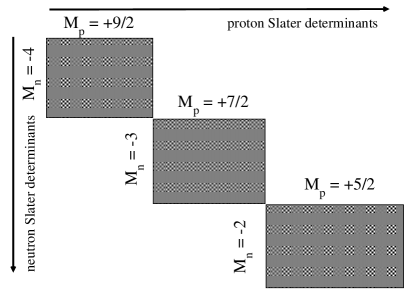
Figure 1: Illustration of factorization of the $M$-scheme many-body basis. Along the $x$-axis we have proton Slater determinants ordered by $M_{p}$, while along the $y$-axis we have neutron Slater determinants also ordered by $M_{n}$ (but in reverse order). Any proton Slater determinant with given $M_{p}$ will combine with any and all neutron Slater determinants with conjugate $M_{n}=M-M_{p}$. Each block therefore represents a sector of the basis in our terminology. This example is for $M=1/2$, taken from the text.

This is an example of factorization. Instead of storing explicitly each and every basis state, one only needs the much smaller set of proton and neutron Slater determinants, and the indexing functions to map to the combined many-body basis. Table 4 gives the number of component proton and neutron Slater determinants for a number of representative cases.

One can also introduce some useful truncations of the many-body basis, also based upon additive weights that act like quantum numbers. In order not to muddy the waters, we give a description of a specific scheme in D.

Table 4: Factorization of the $M$-scheme basis ($M=0$ for even $A$, or $1/2$ for odd $A$) for selected atomic nuclei in terms of the number of proton and neutron Slater determinants needed. The model spaces are described in Appendix B.

Nuclide	space	basis	proton	neutron	$\#$ basis
		dim.	SDs	SDs	sectors
28Si	$sd$	$9.4\times 10^{4}$	924	924	15
56Fe	$pf$	$5.0\times 10^{8}$	38760	184,722	27
56Ni	$pf$	$1.1\times 10^{9}$	$1.2\times 10^{5}$	$1.2\times 10^{5}$	29
6He	$N_{\mathrm{shell}}=6$	$1.4\times 10^{9}$	6216	$6\times 10^{6}$	42
4He	$N_{\mathrm{shell}}=10$	$2.7\times 10^{8}$	96,580	96,580	74
9Li	$N_{\mathrm{max}}=10$	$3.5\times 10^{8}$	$1.5\times 10^{5}$	$1.4\times 10^{7}$	126
9Be	$N_{\mathrm{max}}=10$	$5.7\times 10^{8}$	$1.1\times 10^{6}$	$5.1\times 10^{6}$	136
4He	$N_{\mathrm{max}}=22$	$8.6\times 10^{7}$	$3\times 10^{5}$	$3\times 10^{5}$	307
14C	$N_{\mathrm{shell}}=3$	$2.6\times 10^{8}$	$4\times 10^{4}$	$1\times 10^{5}$	34
12C	$N_{\mathrm{shell}}=4$	$5.9\times 10^{11}$	$4\times 10^{6}$	$4\times 10^{6}$	58
12C	$N_{\mathrm{max}}=8$	$5.9\times 10^{8}$	$5\times 10^{6}$	$5\times 10^{6}$	105

Now that we have introduced the concept of factorization for the basis, we turn to its usage for the interaction.

3 The Hamiltonian and its factorization

In second quantization, a Hamiltonian takes the form

$$\hat{H}=\sum_{ij}T_{ij}\hat{a}^{\dagger}_{i}\hat{a}_{j}+\frac{1}{4}\sum_{ijkl}V_{ijkl}\hat{a}^{\dagger}_{i}\hat{a}^{\dagger}_{j}\hat{a}_{l}\hat{a}_{k}$$ (10)

where $T_{ij}$ are the one-body Hamiltonian matrix elements, which may include kinetic energy and some external or mean-field potential, and $V_{ijkl}$, the two-body matrix elements; as the latter is the primary computational challenge, we ignore the one-body part. One can also add three-body terms, etc., but the underlying principals are unchanged.

The matrix elements are not uncorrelated, due to hermiticity, fermion antisymmetry, and, most germane to this discussion, rotational invariance. The details can be found in standard monographs, e.g. [2]. For our purposes, we only care about selection rules which arise from additive or multiplicative quantum numbers. What this means is, for example, the requirement that, unless

$$m_{i}+m_{j}-m_{k}-m_{l}=0$$

then $V_{ijkl}=0$. This is an example of a conservation law/selection rule. A similar selection rule exists for parity. Below we discuss how we can exploit this for two-species systems, but first, we discuss why the $M$-scheme Hamiltonian matrix is so sparse, and, furthermore, why the nonzero matrix elements have enormous redundancy.

3.1 Sparsity and redundancy of the matrix elements

Table I illustrated the sparsity of $M$-scheme Hamiltonian matrices. This can be understood as arising because we restrict ourselves to a two-body Hamiltonian. We expand upon this idea here.

As explained above, one can represent the basis Slater determinants as binary numbers, with a ‘1’ representing an occupied state and a ‘0’ an occupied state. The action of a destruction operator $\hat{a}_{i}$ is to replace a ‘1’ in the $i$th position with a ‘0’, while a creation operator $\hat{a}^{\dagger}_{i}$ does the opposite:

$$\hat{a}_{4}|01011100\rangle=-|01001100\rangle;$$ (11)

$$\hat{a}^{\dagger}_{4}|01001100\rangle=-|01011100\rangle;$$ (12)

$$\hat{a}_{4}|01001100\rangle=0;\hat{a}^{\dagger}_{4}|01011100\rangle=0.$$ (13)

(The phases arise because of fermion anticommutation relations: every time an annihilation operator anticommutes past a creation operator, we pick up a minus sign.) Trying to create a particle where there already is one gives a zero amplitude; this is the Pauli exclusion principle for fermions. Conversely, trying to destroy a particle where none exists also gives a zero amplitude.

Thus, the action of the operator $\hat{a}^{\dagger}_{i}\hat{a}^{\dagger}_{j}\hat{a}_{l}\hat{a}_{k}$ is to destroy particles in states $k$ and $l$ and put particles in states $i$ and $j$. To simplify, let us assume $i,j,k$, and $l$ are all distinct. Then the amplitude of this operator between two Slater determinants $\mu$ and $\mu^{\prime}$, $\langle\mu^{\prime}|\hat{a}^{\dagger}_{i}\hat{a}^{\dagger}_{j}\hat{a}_{l}\hat{a}_{k}|\mu\rangle$ is zero unless:

$\bullet$ The states $k$, $l$ are occupied in $|\mu\rangle$ and unoccupied in $|\mu^{\prime}\rangle$ ;

$\bullet$ The states $i$, $j$ are occupied in $|\mu^{\prime}\rangle$ and unoccupied in $|\mu\rangle$; and

$\bullet$ all other particles in $|\mu\rangle$ and $|\mu^{\prime}\rangle$ occupy identical states; these are spectators and do not change as one goes from $\mu$ to $\mu^{\prime}$.

As one might imagine, these stringent conditions are difficult to meet; hence, the sparsity found in Table I.

Now the story is not done. Not only is the Hamiltonian matrix sparse, the nonzero matrix elements are furthermore highly redundant. In the action of the Hamiltonian, the operator $\hat{a}^{\dagger}_{i}\hat{a}^{\dagger}_{j}\hat{a}_{l}\hat{a}_{k}$ has a numerical amplitude $V_{ijkl}$. Now this operator will be able to connect many dozens of different pairs of Slater determinants, leading to many dozens of different many-body Hamiltonian matrix elements. But only the spectators differ, while the value of the matrix element $V_{ijkl}$, up to some phase, remains the same.

This leads to large redundancies, as illustrated in Table 5, from factors spanning from 20 to $10^{6}$. In a two-species system, one can devise a factorization algorithm to take partial advantage of this redundancy to reduce the memory load, as described in the following subsections.

Table 5: Some model spaces for atomic nuclei and their $M$-scheme ($M=0$) dimensions and the average redundancy of the Hamiltonian matrix elements (m.e.s), defined as the ratio of the number of nonzero matrix elements (excluding Hermitian conjugates) to the number of unique matrix elements. The model spaces are described in Appendix B.

Nuclide	space	basis	$\#$ nonzero	$\#$ unique	average
		dim	m.e.s	m.e.s	redundancy
28Si	$sd$	$9.4\times 10^{4}$	$2.6\times 10^{7}$	2800	9300
52Fe	$pf$	$1.1\times 10^{8}$	$8.9\times 10^{10}$	$2.2\times 10^{4}$	$4\times 10^{6}$
56Ni	$pf$	$1.1\times 10^{9}$	$1.2\times 10^{12}$	$2.2\times 10^{4}$	$5\times 10^{7}$
4He	$N_{\mathrm{shell}}=8$	$2.9\times 10^{7}$	$1.8\times 10^{11}$	$1.4\times 10^{8}$	1300
4He	$N_{\mathrm{max}}=16$	$6\times 10^{6}$	$2.5\times 10^{10}$	$1.5\times 10^{9}$	18
12C	$N_{\mathrm{shell}}=3$	$8.2\times 10^{7}$	$5.2\times 10^{10}$	$1.6\times 10^{4}$	$3\times 10^{6}$
12C	$N_{\mathrm{max}}=8$	$6\times 10^{8}$	$6.4\times 10^{11}$	$5\times 10^{7}$	$1\times 10^{4}$

3.2 The Hamiltonian with two species

With two species, the Hamiltonian can be written as a sum of different parts

$$\hat{H}=\hat{H}_{x}+\hat{H}_{y}+\hat{H}_{xx}+\hat{H}_{yy}+\hat{H}_{xy}.$$ (14)

Here $\hat{H}_{x}$ is a one-body operator, i.e., kinetic energy plus external potential, that acts only on species x, $\hat{H}_{xx}$ is a two-body operator which denotes the interaction between two particles of species x, and $\hat{H}_{xy}$ is a two-body operator that denotes the interaction between one particle of species x and one particle of species y; the generalizations to species $y$, $\hat{H}_{y}$ and $\hat{H}_{yy}$, are analogous. The one-body terms are easy to work with, so, henceforth, we focus exclusively on the two-body interactions.

We write

$$\hat{H}_{xx}=\frac{1}{4}\sum_{ijkl}V^{(xx)}_{ijkl}\hat{a}^{\dagger}_{i}(x)\hat{a}^{\dagger}_{j}(x)\hat{a}_{l}(x)\hat{a}_{k}(x).$$ (15)

The analogous operator for species $y$, $\hat{H}_{yy}$ has a similar form. The cross-species interaction, that is interaction between a particle of species $x$ and a particle of species $y$, is

$$\hat{H}_{xy}=\sum_{ijkl}V^{(xy)}_{ijkl}\hat{a}^{\dagger}_{i}(x)\hat{a}^{\dagger}_{j}(y)\hat{a}_{l}(y)\hat{a}_{k}(x),$$ (16)

which more broadly can be expanded in a factorized fashion:

$$\hat{H}_{xy}=\sum_{ijkl}V^{(xy)}_{ijkl}\hat{\cal O}^{(x)}_{ik}\hat{\cal O}^{(y)}_{jl}$$ (17)

where, for example,

$$\hat{\cal O}^{(x)}_{ij}=\hat{a}^{\dagger}_{i}(x)\hat{a}_{j}(x).$$ (18)

Because the model space is finite all such expansions are also finite.

Now, we can sketch out the Hamiltonian matrix element (again, considering only the two-body interactions)

$$\langle\nu^{\prime}_{y}|\langle\mu^{\prime}_{x}|\hat{H}|\mu_{x}\rangle|\nu_{y}\rangle=\langle\mu^{\prime}_{x}|\hat{H}_{xx}|\mu_{x}\rangle\delta_{\nu^{\prime}\nu}+\langle\nu^{\prime}_{y}|\hat{H}_{yy}|\nu_{y}\rangle\delta_{\mu^{\prime}\mu}+$$ (19)

$$\sum_{ab}V_{ab}\langle\mu^{\prime}_{x}|\hat{\cal O}^{(x)}_{a}|\mu_{x}\rangle\langle\nu^{\prime}_{y}|\hat{\cal O}^{(y)}_{b}|\nu_{y}\rangle$$

This allows us to begin to see the route to factorization and its efficiency. To begin with, the component matrix elements, $\langle\mu^{\prime}_{x}|\hat{H}_{xx}|\mu_{x}\rangle,\langle\mu^{\prime}_{x}|\hat{\cal O}^{(x)}_{a}|\mu_{x}\rangle$, etc., are much smaller in number than the full matrix elements, as conservation laws/selection rules dramatically restrict the number and coupling of these components.

We assume the Hamiltonian to be rotationally invariant, which means that the Hamiltonian is an angular momentum scalar. (Notice that we also assume the number of particles of each species is conserved, a condition that could be relaxed although it would lead to additional complications.) Because the Hamiltonian commutes not only with $\hat{J}^{2}$ but also $\hat{J}_{z}$, this means that the eigenvalue of $\hat{J}_{z}$, or $M$, is conserved. Earlier, we discussed how this allowed us to invoke a fixed-$M$ basis, which is easy to construct using Slater determinants. But now we go further: because the interaction cannot change $M$, in Eqs. (15) and (16) we have

$$m_{i}+m_{j}-m_{k}-m_{l}=0.$$ (20)

Similarly for parity,

$$\pi_{i}\times\pi_{j}\times\pi_{k}\times\pi_{l}=+1.$$ (21)

The conservation of these quantum numbers dramatically restricts the number and the coupling of the matrix elements, as we will now lay out.

3.3 Two-body jumps

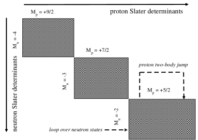
Figure 2: Illustration of factorization of $H_{pp}$ for the example in the text. Because the conjugate neutron Slater determinant does not change, the ‘two-body jump’ cannot change either $M_{n}$ or $M_{p}$. Instead we loop over all (proton) two-body jumps and also loop over all conjugate (neutron) Slater determinants.

Consider $\hat{H}_{xx}$, the interaction between two particles of species $x$; $\hat{H}_{yy}$ works exactly the same. As described above,

$$\langle\nu^{\prime}_{y}|\langle\mu^{\prime}_{x}|\hat{H}_{xx}|\mu_{x}\rangle|\nu_{y}\rangle=\langle\mu^{\prime}_{x}|\hat{H}_{xx}|\mu_{x}\rangle\delta_{\nu^{\prime}\nu}.$$ (22)

What does this mean for computing the matrix element of $\hat{H}_{xx}$? Because $\nu=\nu^{\prime}$ for the $y$-basis component, $\hat{H}_{xx}$ cannot change $M_{y}$ or $\Pi_{y}$, which in turn means that it cannot change $M_{x}$ or $\Pi_{x}$. Figure 2 gives a schematic version.

Thus, although we need the $\langle\mu^{\prime}_{x}|\hat{H}_{xx}|\mu_{x}\rangle$, we only need them diagonal in quantum numbers such as $M_{x}$, which enormously reduces the amount of information. The $\langle\mu^{\prime}_{x}|\hat{H}_{xx}|\mu_{x}\rangle$ are called ‘two-body jumps.’ Each two-body jump consists of the following information:

$\bullet$ the initial $x$-state label $\mu$;

$\bullet$ the final $x$-state label $\mu^{\prime}$;

$\bullet$ and the value of the matrix element $\langle\mu^{\prime}_{x}|\hat{H}_{xx}|\mu_{x}\rangle$ (which includes a phase $\pm 1$ from fermion anticommutation).

These ‘jumps’ can be stored as simple arrays, along with indexing information that tells us the start and stop points for two-body jumps for a given $M_{x}$ etc. Because the jumps are at the heart of the factorization algorithm, they are best kept as simple arrays; storing within derived types in modern Fortran, for example, can increase run time by a factor of two.

The application of $\hat{H}_{xx}$ is given below in pseudocode. It is helpful to remind ourselves of what we learned about the factorization of the basis in Section 2.2: any $x$-basis state $|\mu_{x}\rangle$ has quantum numbers $M_{x}$, $\Pi_{x}$ (and optionally the ‘weighting’ $W_{x}$, used for many-body truncations, as discussed in D); the subset of $x$-states $|\mu_{x}\rangle$ with the same quantum numbers is called a sector, which in the pseudocode we label by $\Gamma_{x}$. A $y$-sector $\Gamma_{y}$ is ‘conjugate’ to $\Gamma_{x}$ if $M_{x}+M_{y}=M$, the fixed total $J_{z}$ for the calculation, and $\Pi_{x}\times\Pi_{y}=\Pi$ and $W_{x}+W_{y}\leq W_{\mathrm{max}}$. Furthermore, as in Eqn. 9 there exist index function $f_{x}(\mu_{x})$ and $f_{y}(\nu_{y})$ whose sum gives us the index $\alpha$ of the combined basis state.

Then the pseudocode is:

FOR all $x$-sectors $\Gamma_{x}$

FOR all the $x$-species two-body jumps $\in\Gamma_{x}$

Fetch $\mu_{x}$, $\mu_{x}^{\prime}\in\Gamma_{x}$ and

Fetch matrix element $\langle\mu^{\prime}_{x}|\hat{H}_{xx}|\mu_{x}\rangle$ from the jumps arrays

FOR all $\Gamma_{y}$ conjugate to $\Gamma_{x}$

FOR all $\nu_{y}\in\Gamma_{y}$

$\alpha_{i}=f_{x}(\mu_{x})+f_{y}(\nu_{y})$

$\beta_{f}=f_{x}(\mu^{\prime}_{x})+f_{y}(\nu_{y})$

$v_{f}(\beta_{f})=v_{f}(\beta_{f})+v_{i}(\alpha_{i})\times\langle\mu^{\prime}_{x}|\hat{H}_{xx}|\mu_{x}\rangle$

$v_{f}(\alpha_{i})=v_{f}(\alpha_{i})+v_{i}(\beta_{f})\times\langle\mu^{\prime}_{x}|\hat{H}_{xx}|\mu_{x}\rangle^{*}$ (hermiticity)

END FOR

END FOR

END FOR

END FOR

In a purely serial code lookup of the jump information is time consuming, and so looping over the spectator $y$-states is best as the innermost loop, but for example when using OpenMP or other shared-memory parallel schemes, we use the loop over the spectator $y$-states the outer loop in order to avoid data collisions.

To illustrate this algorithm, we return to the example given in Section 2.2, and in particular in Table 3. The proton-proton or $xx$ part of the Hamiltonian cannot change $M_{n}$ and so also cannot change $M_{p}$. Now let’s consider the specific case of the sector of the basis with $M_{p}=+5/2$ and $M_{n}=-2$. There are a total of 8720 basis states in this sector, so there are possibly $8720^{2}=68\times 10^{6}$ matrix elements. However, $\hat{H}_{pp}$ cannot change the neutron Slater determinant, so that, as in Eq. (22), $\nu=\nu^{\prime}$.

Now in this sector, there are 80 proton Slater determinants $|\mu_{p}\rangle$ with $M_{p}=5/2$, so that in principle there could be $80^{2}=6400$ matrix elements $\langle\mu^{\prime}_{p}|\hat{H}_{pp}|\mu_{p}\rangle$ (or half that if we take into account hermiticity). But we have a two-body interaction and five particles, so that for each nonzero matrix element there are always three static spectators. This reduces the number of nonzero matrix elements of $\langle\mu^{\prime}_{p}|\hat{H}_{pp}|\mu_{p}\rangle$ to 2677.

With the two-body jumps in hand, we can easily reconstruct the full matrix element, Eq. (22), for this sector of the basis. We loop over all 2677 two-proton jumps, which takes us from one proton Slater determinant $|\mu_{p}\rangle$ to another $|\mu^{\prime}_{p}\rangle$, including the value of the matrix element. We also have a fast, inner loop over the 109 neutron Slater determinants $|\nu_{y}\rangle$ which do not change. (Note: if we parallelize our code with memory sharing, e.g. with OpenMP, it is useful to either make the loop over $\nu_{y}$ the outer loop or to order the jumps based on the index of the final state and sort on thread boundaries in order to avoid data collisions.) We invoke the straightforward indexing of the basis, Eq. (9), to obtain the indices of the initial and final basis states. End result: out of a possible 68 million matrix elements in this sector, we use just 2677 two-proton jumps to find the $2677\times 109=291793$ nonzero matrix elements (a sparsity of $0.4\%$). (Furthermore, there are only 350 unique values of the matrix elements.) This illustrates how factorization can compress, without approximation, an already very sparse matrix into a relatively small amount of memory.

Table 6: Number of one- and two-body ‘jumps’ and storage requirements for representative atomic nuclei in different model spaces (described in Appendix B). For storage of nonzero matrix elements (penultimate column) we assume each many-body matrix element is stored by a 4-byte real number and its location encoded by a single 4-byte integer. Storage of a single jump (initial and final Slater determinants for a species, and matrix element and phase) requires 13 bytes. All storage (final two columns) are in gigabytes (GB).

Nuclide	space	basis	$\#$ 1-body	$\#$ 2-body	Store	Store
		dim	jumps	jumps	m.e.s	jumps
28Si	$sd$	$9.4\times 10^{4}$	$4.8\times 10^{4}$	$7.6\times 10^{3}$	0.2	0.002
52Fe	$pf$	$1.1\times 10^{8}$	$4.0\times 10^{6}$	$8.5\times 10^{6}$	700	0.16
56Ni	$pf$	$1.1\times 10^{9}$	$1.5\times 10^{7}$	$4.0\times 10^{7}$	9800	0.6
4He	$N_{\mathrm{shell}}=8$	$2.9\times 10^{7}$	$1.4\times 10^{7}$	$2.9\times 10^{7}$	1500	0.6
4He	$N_{\mathrm{max}}=22$	$9\times 10^{7}$	$5.3\times 10^{8}$	$4.7\times 10^{9}$	9300	69
12C	$N_{\mathrm{shell}}=3$	$8.2\times 10^{7}$	$4\times 10^{6}$	$7\times 10^{6}$	400	0.14
12C	$N_{\mathrm{shell}}=4$	$6\times 10^{11}$	$8\times 10^{8}$	$2.4\times 10^{9}$	$10^{7}$	43
12C	$N_{\mathrm{max}}=8$	$6\times 10^{8}$	$6\times 10^{8}$	$3\times 10^{9}$	5200	45
13C	$N_{\mathrm{max}}=6$	$3.8\times 10^{7}$	$7\times 10^{7}$	$3\times 10^{8}$	210	4.3

Comparison between storage scheme and factorization is given in Table 6 and discussed below in Subsection 3.6.

3.4 One-body jumps

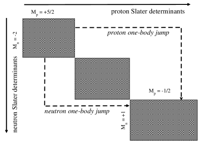
Figure 3: Illustration of factorization of $H_{pn}$ using one-body jumps, for the example in the text. The change in $M_{p}$ must be matched by the change in $M_{n}$.

The action of $\hat{H}_{xy}$ is more complicated: it moves one particle of species $x$ and one particle of species $y$. Nonetheless, factorization is still viable, and, in fact, it greatly reduces the memory storage requirements.

Using Eq. (17), the matrix element of $\hat{H}_{xy}$ is

$$\langle\nu^{\prime}_{y}|\langle\mu^{\prime}_{x}|\hat{H}_{xy}|\mu_{x}\rangle|\nu_{y}\rangle=\sum_{ab}V_{ab}\langle\mu^{\prime}_{x}|\hat{\cal O}^{(x)}_{a}|\mu_{x}\rangle\langle\nu^{\prime}_{y}|\hat{\cal O}^{(y)}_{b}|\nu_{y}\rangle$$ (23)

We call $\langle\mu^{\prime}_{x}|\hat{\cal O}^{(x)}_{a}|\mu_{x}\rangle$ and $\langle\nu^{\prime}_{y}|\hat{\cal O}^{(y)}_{b}|\nu_{y}\rangle$ one-body jumps for species $x$ and $y$, respectively. Like two-body jumps, for each one-body jump we must store the labels of the initial and final Slater determinants plus the label $a$ of the one-body operator $\hat{\cal O}_{a}$.

Because neither the $x$ nor the $y$ Slater determinants are spectators, individual quantum numbers such as $M_{x}$ and $M_{y}$ are no longer constant. On the other hand, because the total $M=M_{x}+M_{y}$ is constant, we know that $M_{y}$ must change in an equal and opposite manner to the change in $M_{x}$.

So, going back to our example from the previous subsection (Table 3), if we start in the sector $M_{p}=+5/2$, $M_{n}=-2$, if the proton one-body jump takes us to $M_{p}=-1/2$ then we must have a conjugate neutron one-body jump that takes us to $M_{n}=+1$. Figure 3 gives a schematic version.

For $H_{xx}$, we looped over the 2-body jumps of species $x$ and then had a simple loop over the allowed conjugate states of species $y$ dictated by quantum numbers. For $H_{xy}$, we must first identify the initial and final $M$-scheme sectors, and loop over all the associated one-body $x$-jumps and all the conjugate one-body $y$-jumps. The pseudocode is:

FOR all initial $\Gamma^{i}_{x}$, all final $\Gamma^{f}_{x}$

FOR all $\Gamma^{i}_{y}$ conjugate to $\Gamma^{i}_{x}$, $\Gamma^{f}_{y}$ conjugate to $\Gamma^{f}_{x}$

FOR all $x$-jumps $\in\Gamma^{i}_{x}\rightarrow\Gamma^{f}_{x}$, all $y$-jumps $\in\Gamma^{i}_{y}\rightarrow\Gamma^{f}_{y}$,

Fetch $\mu_{x}\in\Gamma^{i}_{x},\mu_{x}^{\prime}\in\Gamma^{f}_{x}$

Fetch $\nu_{y}\in\Gamma^{i}_{y},\nu_{y}^{\prime}\in\Gamma^{f}_{y}$

Fetch $\langle\mu_{x}^{\prime},\nu_{y}^{\prime}|H|\mu_{x},\nu_{y}\rangle$

$\alpha_{i}=f_{x}(\mu)+f_{y}(\nu)$;

$\beta_{f}=f_{x}(\mu^{\prime})+f_{y}(\nu^{\prime})$

$v_{f}(\beta_{f})=v_{f}(\beta_{f})+v_{i}(\alpha_{i})\langle\mu_{x}^{\prime},\nu_{y}^{\prime}|H|\mu_{x}\nu_{y}\rangle$

$v_{f}(\alpha_{i})=v_{f}(\alpha_{i})+v_{i}(\beta_{f})\langle\mu_{x}^{\prime},\nu_{y}^{\prime}|H|\mu_{x}\nu_{y}\rangle^{*}$ (hermiticity)

END FOR

END FOR

END FOR

(Again: an $x$-sector, labeled $\Gamma_{x}$, is a subset of $x$-species Slater determinants with fixed quantum numbers $M_{x}$, $\Pi_{x}$, while $\mu_{x},\nu_{y}$ label $x$-species and $y$-species Slater determinants, respective, and $\alpha_{i}$ is the index of the many-body basis state constructed by the product of those two Slater determinants.)

Going from the subspace (or sector) $M_{p}=5/2,M_{n}=-2$ (dimension 8720) to the sector $M_{p}=-1/2$, $M_{n}=1$ (dimension 15,232) the number of possible matrix elements is $8720\times 15,232=1.3\times 10^{8}$; but there are 337 proton jumps and 419 neutron jumps and a total of $337\times 419=132,823$ nonzero matrix elements, with a sparsity of $0.1\%$.

Again, comparison between storage scheme and factorization is given in Table 6 and discussed below in Subsection 3.6.

3.5 Three-body forces

One can generalize in a straightforward manner the previous algorithm to three-body forces. Here, one now has $H_{xxx}$, $H_{xxy}$, $H_{xyy}$, and $H_{yyy}$. The first and the last require ‘three-body jumps,’ while $H_{xxy}$ and $H_{xyy}$ require combining one- and two-body jumps. In Table 7, we compare, for three-body forces, the sparsity as well as the memory requirements to store the nonzero matrix elements and to store the jumps; these can be compared to data in Tables 1 and 6. The matrices are, as expected, significantly less sparse, while we retain the significant memory efficiency by storing jumps rather than storing the nonzero matrix elements.

Table 7: Storage requirements for three-body interactions for representative atomic nuclei in different model spaces (described in Appendix B). The corresponding data for two-body interactions can be found in Tables 1 and 6. All storage (final two columns) are in gigabytes (GB).

Nuclide	space	basis	Sparsity	Store	Store
		dim		m.e.s	jumps
28Si	$sd$	$9\times 10^{4}$	0.06	2.1	0.01
52Fe	$pf$	$1\times 10^{8}$	$3\times 10^{-4}$	$1.5\times 10^{4}$	1.6
4He	$N_{\mathrm{shell}}=8$	$3\times 10^{7}$	0.03	$1.2\times 10^{5}$	11
4He	$N_{\mathrm{max}}=14$	$2\times 10^{6}$	0.10	2000	16
12C	$N_{\mathrm{shell}}=3$	$8\times 10^{7}$	$3\times 10^{-4}$	8800	1.4
13C	$N_{\mathrm{max}}=6$	$4\times 10^{7}$	$1\times 10^{-3}$	6200	80
12C	$N_{\mathrm{max}}=8$	$6\times 10^{8}$	$1.5\times 10^{-4}$	$2\times 10^{5}$	1100

3.6 Comparison of memory requirements

Using ‘jumps’ to store the information about the many-body Hamiltonian matrix elements is significantly more efficient than storing the matrix elements, as illustrated for two-body interactions in Table 6: the memory requirements are 50 to 100 times less for factorization, an enormous savings. Furthermore, reconstruction of the matrix elements is very fast; in timing tests it is no more than a factor of two slower than simply fetching the matrix element from memory, and that is for $H_{xy}$; for $H_{xx/yy}$ the timing between factorization and storage is similar. Table 7 makes the comparison for three-body forces, where the ratio is even larger.

There are other advantages. Setup of the arrays is very fast, especially if one takes the method further as we describe in the next section. Because we can ‘forecast’ the number of operations without actually creating or directly counting the nonzero matrix elements, we can quickly obtain that information and distribute the work for parallel processing, as we describe in Section 5.

The take-away lesson is: while the $M$-scheme Hamiltonian matrix is very sparse, one can dramatically reduce the storage requirements further by one or two orders of magnitude using factorization; in the case of three-body forces, the reduction can be as high as three orders of magnitude. With factorization one can run efficiently on a desktop machine problems that would otherwise require storing the many-body Hamiltonian on disk, with slow I/O, or distributing the matrix elements across many compute nodes on a distributed memory parallel machine. Alternately, on the same parallel machine one could tackle a much larger problem–50 or 100 times larger, even more in the case of three-body forces as discussed in Subsection 3.5 – than with a matrix storage scheme. Thus, despite the higher intrinsic complexity of the algorithm (and we note that leadership class codes using matrix storage are by no means ‘simple’), factorization can, using the same computational resources, push the limits of calculations further.

4 Factorization: the next step

Inspired by ANTOINE [18], our first attempt at on-the-fly CI code was REDSTICK (unpublished), initiated while two of us (CWJ and WEO) were at Louisiana State University in Baton Rouge, La. When we began to plan our next generation code, BIGSTICK, we first looked at the computational bottlenecks in REDSTICK. They were, in decreasing order of importance:

$\bullet$ Inefficient application of the jumps when making truncations on the many-body space (briefly: use of the $W$ weighting index to truncate the many-body space, as described in D, further restricts application of the jumps, but this was not handled in an efficient manner);

$\bullet$ Inefficient distribution of the matvec (matrix-vector multiply) operations across parallel computational nodes;

$\bullet$ Inefficient generation of the basis, especially for large relative truncation based on weighting $W$; and

$\bullet$ Inefficient generation of the one- and two- (and, for three-body interactions, three-) body jumps. Note that no other on-the-fly CI code has 3-body capabilities; this was our major motivation for writing REDSTICK and BIGSTICK.

The first bottleneck, inefficient application of the jumps, was addressed by organizing both the basis and the jumps by sectors, that is, labeling by $M,\Pi$ and $W$. The second bottleneck, inefficient parallelization, we address below in Section 5. The final two bottlenecks we addressed by introducing a new level of factorization.

As described above, the basis is factorized into a product of $x$- and $y$-species Slater determinants (e.g. proton and neutron Slater determinants, or up- and down-spin electron Slater determinants) which have conjugate quantum numbers. We have taken this strategy to the next level. Each Slater determinant for given species is itself written as a product of two ‘half-Slaters,’ one constructed from single-particle states with $m<0$, and the other from single-particle states with $m\geq 0$.

$$|\mu_{x}\rangle=|\omega^{(L)}_{x}\rangle|\omega^{(R)}_{x}\rangle.$$ (24)

Here ‘L’ denotes a ‘left’ half-Slater determinant (hSD) , constructed with single-particle states with $m<0$, ‘R’ denotes a ‘right’ hSD constructed with single-particle states with $m\geq 0$, and $\omega^{(L),(R)}$ denotes the quantum numbers associated with each hSD, notably $M^{(L),(R)}$, $\Pi^{(L),(R)}$, $W^{(L),(R)}$, and, crucially, the number of particles $n^{(L),(R)}$. As usual, $M_{x}=M^{(L)}+M^{(R)}$, etc, while $n_{x}=n^{(L)}+n^{(R)}$. Any full basis state is now the product of four half-Slater determinants, e.g. $|\alpha\rangle=|\omega^{(L)}_{x}\rangle|\omega^{(R)}_{x}\rangle|\omega^{(L)}_{y}\rangle|\omega^{(R)}_{y}\rangle$. However this combining is only done implicitly and never explicitly.

Crucially, and unlike the Slater determinants of species $x$ and $y$, these half-Slater determinants do not have fixed particle number, which now acts as a new quantum number. While this adds a layer of complexity, it also offers several advantages. In the same way one constructs a very large total basis from much smaller lists of $x$- and $y$- Slater determinants, the number of required hSDs is much smaller still. For any given set of quantum numbers $n$, $M$, $\Pi$ (and $W$), the list of half-Slaters is small. Examples are given in Table 8; one gets bigger savings for more particles and for full-configuration bases.

Table 8: Factorization of the $M$-scheme basis ($M=0$) for selected atomic nuclei in terms of the number of ’half-Slater determinants’.

Nuclide	space	basis	proton	proton
		dim.	SDs	hSDs
28Si	$sd$	$9.4\times 10^{4}$	924	128
52Fe	$pf$	$1.1\times 10^{8}$	38760	1696
56Ni	$pf$	$1.1\times 10^{9}$	$1.2\times 10^{5}$	2026
4He	$N_{\mathrm{shell}}=8$	$2.9\times 10^{7}$	28,680	1522
4He	$N_{\mathrm{max}}=22$	$8.6\times 10^{9}$	$3.3\times 10^{5}$	$2.8\times 10^{5}$
12C	$N_{\mathrm{shell}}=4$	$5.9\times 10^{11}$	$4\times 10^{6}$	$1\times 10^{5}$
12C	$N_{\mathrm{max}}=8$	$5.9\times 10^{8}$	$3\times 10^{6}$	$6\times 10^{5}$

Furthermore, the fact that the half-Slaters do not have fixed particle number becomes an advantage. We do not always need all possible Slater determinants of a given species, but merely all Slater determinants of a fixed set of quantum numbers.

For example, consider severe many-body truncations based upon the $W$-weighting described in D, where one forces the sum of weights associated with single-particle states to be less than some value. In this case, generating the required Slater determinants, is a nontrivial task. Generating all possible Slater determinants and eliminating those unneeded turns out to be horribly inefficient. For example, consider a $W=2$ cut on ¹⁶O. There are only 1245 proton Slater determinants needed to construct the basis, but if one naively generated all Slater determinants in the single-particle space there would be 76 million Slater determinants.

The answer, of course, is instead of generating millions or billions of candidate Slater determinants and throwing away the bulk of them, one creates them recursively: start by creating one-particle states, then two-particle states, and so on, and by constraining the additive quantum numbers one can arrive at the required basis. This was done, for example, in our first generation code, REDSTICK. But even so, this is somewhat wasteful, as one throws away the intermediate basis sets.

The half-Slaters answer this: not only do we construct the half-Slaters recursively (from the vacuum state we generate all the needed one-particle half-Slaters, and from the one-particles half-Slaters we generate all the two-particle half-Slaters, and so on), we actually need all or most of these hSDs in order to create the Slater determinants. Furthermore, this gives us a route to creating the ‘jumps.’

Let us explain in more detail. First, we break the single-particle space, for example that found in Table 2. The single-particle states 1, 3, 5, 7, 8, and 9, which all have $m_{j}<0$, are grouped together (as ‘left’ or L states), while the remaining single particle states with $m_{j}>0$ are group as ’right’ or R states. Let’s focus first on the left states. We start with the vacuum: 000000. From the vacuum state we create six one-particle hSDs: 100000, 010000, 001000, etc. From each of the one-particle hSDs we create two-particle hSDs; one can do this without duplication by only adding a particle to the right of all filled states, that is,

$$001000\rightarrow 001100,001010,001001$$

and so on, recursively. If one is making a cut on the many-body basis using the $W$ weighting, one simply does not create hSDs that would violate the maximum $W$ allowed.

Almost for free we have the action of creation operators on a half-Slater, that is, the matrix element

$$\langle\omega^{\prime}|\hat{a}^{\dagger}_{i}|\omega\rangle,$$ (25)

where $n_{\omega^{\prime}}=n_{\omega}+1$. We call such a matrix element a ‘hop’ and it comes out automatically when generating all the half-Slaters with $n_{\omega}+1$ particles from the half-Slaters with $n_{\omega}$ particles. In practice, we sort the hSDs, already grouped by the number of particles $n_{\omega}$, by $M_{\omega},\Pi_{\omega},W_{\omega}$; because the lists are small, the sorting is quick. Then when computing the ‘hop’ we know the initial and final quantum numbers and the search through the list of possible final states is also very quick. It is this kind of sorting and searching that is most time-consuming in occupation-space CI codes, and by breaking down the basis into half-Slaters, and thus making all lists to be sorted and searched much smaller, we speed up the process considerably.

There are typically a small number of these ‘hops’ and they are, again, organized efficiently by quantum numbers; in fact, given the quantum numbers associated with $\omega$ and $\omega^{\prime}$ the quantum number of the single-particle state $i$ is fixed. Some illustrative data on hops is found in Table 9.

Table 9: Construction of the many-body matrix elements (for two-body interactions) via creation-operator ‘hops.’ For three-body interactions, the number of jumps and many-body matrix elements will increase, but the number of hops is fixed.

Nuclide	space	# nonzero	#	#
		many-body m.e.s	jumps	hops
28Si	$sd$	$2.6\times 10^{6}$	$1.2\times 10^{5}$	768
52Fe	$pf$	$8.9\times 10^{10}$	$1.2\times 10^{7}$	15280
56Ni	$pf$	$1.2\times 10^{12}$	$5.6\times 10^{7}$	20080
4He	$N_{\mathrm{shell}}=8$	$1.8\times 10^{11}$	$4.3\times 10^{7}$	$6\times 10^{4}$
4He	$N_{\mathrm{max}}=22$	$1.1\times 10^{12}$	$5.3\times 10^{9}$	$1.5\times 10^{6}$
12C	$N_{\mathrm{shell}}=3$	$5\times 10^{10}$	$1\times 10^{7}$	$1.5\times 10^{4}$
12C	$N_{\mathrm{shell}}=4$	$1.5\times 10^{15}$	$3.3\times 10^{9}$	$1.3\times 10^{6}$
12C	$N_{\mathrm{max}}=8$	$6.4\times 10^{11}$	$3.4\times 10^{9}$	$4.2\times 10^{6}$

From the hops one can then build one- and two-body jumps needed for the action of the Hamiltonian. The algorithm for doing so is slightly involved, but it is quick, because one has dramatically reduced searches. For example, to generate all the jumps needed for ⁵²Fe in the $pf$ shell, it takes less than 30 seconds on a standard desktop machine–and each matrix multiplication takes more than 30 minutes. (For large $W$ cuts, the efficiencies drop; the number of half-Slaters needed relative to the final basis dimension is larger, and the time to generate jumps is also longer.)

In going from REDSTICK, which has a single level of factorization, to BIGSTICK, which by exploiting hSDs has two levels of factorization, basis construction speeds up consistently by a factor of 3-4 times, while construction of jumps speeds up consistently by a factor of 10, independent of dimensionality.

To describe the construction of jumps from hops, we have to introduce a few more concepts. Along the way, we continue to organize everything by quantum numbers $m,\pi,w$. This shortens lists to be searched.

Suppose we want to build $n$-body jumps, which is the action of $n$ annihilation operators followed by $n$ creation operators, e.g. $\hat{a}^{\dagger}\hat{a}^{\dagger}\ldots\hat{a}\hat{a}$. As an intermediate step, we consider $n$-particle hops, which simply chain together $n$ annihilation hops removing $n$ particles. Applying an $n$-body annihilation hop to a sector $\Gamma$ creates a new, intermediate sector, $Q$, with $n$ fewer particles, and so is not part of the basis, but is constructed with half-Slater determinants already created.

The key idea, outlined below in pseudocode, is to construct $n$-particle hops from both initial and final sectors, $\Gamma^{i},\Gamma^{f}$, to the same intermediate sector $Q$. Then, by looping over states $q$ in $Q$, we can work backwards and find the initial and final states in $\Gamma^{i},\Gamma^{f}$ and construct the jumps.

FOR all initial sector $\Gamma^{i}$

Find all allowed $Q$ from subtracting $n$ particles

FOR all $Q$

Find all $n$-body hops $\Gamma^{i}\rightarrow Q$

FOR all final sectors $\Gamma^{f}$

Find all $n$-body hops $\Gamma^{f}\rightarrow Q$

FOR all intermediate states $q\in Q$

Find all initial $\mu\in\Gamma^{i}$, such that $\mu\rightarrow q$

Find all all final $\mu^{\prime}\in\Gamma^{f}$, such that $\mu^{\prime}\rightarrow q$

Create $n$-body jump(s) $\mu\rightarrow\mu^{\prime}$

END FOR

END FOR

END FOR

END FOR

Because the hops carry information about the fermion creation and annihilation operators, that information is automatically inherited by jumps, allowing one to find the appropriate matrix element.

Parceling the basis and the interaction also allows for rather fine control for parallel work, as discussed in detail in the next section.

5 Parallelization and load balancing

All the CI codes described in this paper follow Whitehead’s pioneering use of the Lanczos algorithm to efficiently find low-lying eigenstates[13]. (Another popular algorithm is Davidson-Liu and its variants [27, 28], designed primarily for diagonal-dominant matrices, a context appropriate for atomic physics but not nuclear.) The central operation in the Lanczos algorithm is a matrix-vector multiplication (matvec). Since for an $M$-scheme basis the Hamiltonian many-body matrix is very sparse, the key to efficient parallelization and load balancing of the matvec operation is to distribute as evenly as possible the nonzero matrix elements across the compute nodes.

In our first-generation code, REDSTICK, we distributed the matvec operations by initial basis state. Each basis state, however, has vastly different numbers of operations connection to it. Fig. 4 illustrates this for the case of ⁶Li in an $N_{\mathrm{max}}=6$ space (two-body interactions only); Fig. 5 shows on a log graph the same information but sorted. Thus, naively distributing work by basis state lead to unbalanced workloads. Sorting as in Fig. 5 will not help to balance workloads as “nearby” initial states connect to very different final states.

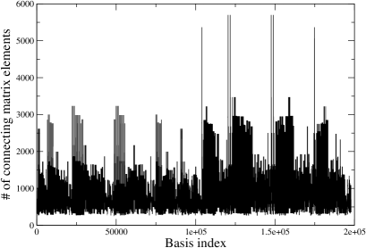
Figure 4: For ⁶Li in $N_{\mathrm{max}}=6$ space (dimension = 197,822), number of matrix elements connecting to each basis state.

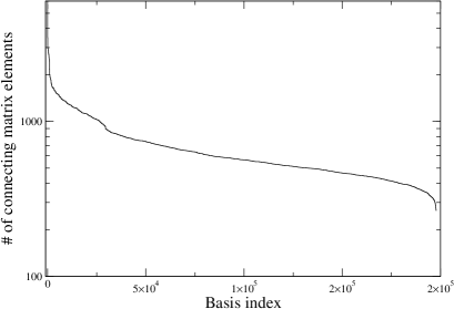
Figure 5: The same as Fig. 4, but sorted on the number of connecting matrix elements..

The partial grouping can be understood as related to organizing the basis into sectors labeled by quantum numbers of the proton Slater determinants. When storing matrix elements on core, one can average this out through a randomizing, ‘round-robin’ algorithm [29]. Such a method will not work when using quantum numbers to factorize the Hamiltonian, however.

While investigating the distribution of the matvec operations, we realized that factorization itself gives us the key to parallelization. As explained in section III, the Hamiltonian is a sum of one- and two-body terms. Since it is easy to work with the one-body terms, here we focus on the parallelization of the application of the two-body terms, i.e., $\hat{H}_{xx}$, $\hat{H}_{yy}$, and $\hat{H}_{xy}$. The action of these operators is organized in one- and two-body jumps. The key to efficient parallelization of BIGSTICK is to distribute the jumps across parallel cores in such a way that each compute core performs (approximately) equal number of operations as described below. (A ‘core’ is either a MPI process, in a pure MPI distributed memory programming model, or a thread, in an OpenMP shared memory programming model, or a hybrid MPI+OpenMP programming model.)

Rather than counting up operations individually to/from each state, we break up the Hamiltonian into blocks based upon quantum numbers, that is, we organize Hamiltonian operations by the initial and final sectors of the basis (where a ‘sector’ of the basis is labeled by the quantum number $M_{x},\Pi_{x},W_{x}$ of the $x$-species). In this way, we can compute the number of operations without actually counting them individually. In the example discussed in Section III.C, we know from 2677 proton two-body jumps and 109 conjugate neutron Slater determinants, that we get $2677\times 109=291,793$ operations. It is these ‘blocks’ of operations, based upon quantum numbers, that we break up and distribute across compute cores, with fairly modest bookkeeping.

For instance, continuing the same example, suppose we find we want approximately 100,000 operations per compute core. For the block of operations in our example, we can have proton two-body jumps number 1 through 917 on the first compute core, jumps 918 through 1834 on the second compute core, and 1835 through 2677 on the third compute core. Each core loops over all 109 conjugate neutron Slater determinants.

We find this distribution of the matrix-vector multiplication scales very well. Fig. 6 demonstrates scaling from 64 to 4096 cores for the case of ⁵⁰Mn in the $pf$ shell (basis dimension of 18 million) with a three-body force; the data was taken on the Jaguar supercomputer at Oak Ridge National Laboratory in September 2012. We have done a number of similar studies; for example, with an earlier version of BIGSTICK we found similar scaling of the matvec operation from 500 to 10000 cores on the Franklin machine at the National Energy Research Computing Center (NERSC) for ⁵²Fe in the $pf$ shell (dimension 110 million) with a two-body interaction.

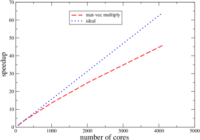
Figure 6: (Color online) Relative speed-up of the matvec operation for ⁵⁰Mn in the $pf$-shell, with an $M$-scheme dimension of $1.8\times 10^{7}$ with three-body interactions. Solid (black) line corresponds to the ideal speed-up and broken (red) line to the actual speed-up. Data from Jaguar at Oak Ridge National Laboratory in September 2012.

At this point the major computation bottlenecks are communication and, if one writes the Lanczos vectors to disk, I/O (alternately, one can store the Lanczos vectors also across many compute nodes[29]). All parallel CI codes face these same barriers.

6 Summary and Conclusion

Configuration-interaction calculations of the many-fermion problem are straightforward: one diagonalizes the Hamiltonian in a many-body basis. If that basis is made of Slater determinants with fixed $J_{z}$, the resulting matrix is very sparse; despite the sparsity, however, the number of nonzero matrix elements quickly becomes overwhelming (cf. Table 1). Investigation of the nonzero matrix elements reveals a high degree of redundancy, that is, the same numerical value of the matrix element, up to a phase, over and over again (cf. Table 5).

Both the sparsity and the redundancy can be understood as the consequence of having a two- or three-body interaction embedded in a many-body space, with a consequence of many spectator particles. Nonetheless, while the sparsity reduces the number of many-body matrix elements, simply determining the nonzero matrix elements–often of the order of just one in a million–is a nontrivial problem.

That very sparsity, however, can be turned to an advantage. In this paper, we discussed how, if one has two species of particles and if there are abelian quantum numbers (which simply means the quantum numbers are additive or multiplicative), one can further compactify the problem via factorization. Factorization yields a memory savings of one to almost three orders of magnitude, as shown in Tables 6,7; furthermore, it can make planning of the parallel distribution of work straightforward, as one can calculate the number of operations without explicitly constructing them. While factorization has been used in nuclear physics codes for well over a decade, recent work taking factorization an additional step leads to additional efficiencies. There is a cost to all this, of course, in more complicated internal bookkeeping. It is worth pursuing, however, as it will allow us to tackle significantly larger problems, than a straight matrix storage scheme, on the same computing platform.

The U.S. Department of Energy supported this investigation through contracts DE-FG02-96ER40985 and DE-FC02-09ER41587, and through subcontract B576152 by Lawrence Livermore National Laboratory under contract DE-AC52-07NA27344. We would like to thank H. Nam, J. Vary, and P. Maris for helpful conversations over the years regarding the development of CI codes.

Appendix A Quantum numbers

In this section, we briefly introduce the concept of quantum numbers for non-physicists (e.g., computer scientists and applied mathematicians).

Quantum numbers label irreducible representations of a group. In quantum mechanics, the labeling is done using eigenvalues of commuting operators [30]; often these eigenvalues in turn correspond to physically conserved quantities, especially if the group is continuous.

In classical mechanics, Noether’s theorem states that if a Hamiltonian is invariant under an operation, there will be a corresponding conserved quantity. Invariance under spatial translation leads to conservation of linear momentum, while invariance under spatial rotation leads to conservation of angular momentum.

In quantum mechanics, any observable quantity that can be measured is represented by a Hermitian, linear operator $\hat{\cal O}$; the allowed values that can be measured are the eigenvalues of the operator,

$$\hat{\cal O}|\Psi\rangle=\lambda|\Psi\rangle.$$ (26)

Invariance in quantum mechanics is given by commutation: if $[\hat{H},\hat{\cal O}]=0$, then one can have simultaneous eigenstates:

$$\hat{H}|E,\lambda\rangle=E|E,\lambda\rangle,\,\,\,\,\hat{\cal O}|E,\lambda\rangle=\lambda|E,\lambda\rangle.$$ (27)

In this case, $\lambda$ corresponds to a conserved quantity: this value does not change under the evolution of the wavefunction through the time-dependent Schödinger equation. For many important conserved quantities, such as total angular momentum

$$\hat{J}^{2}|\Psi\rangle=j(j+1)\hbar^{2}|\Psi\rangle$$ (28)

and the $z$-component of angular momentum

$$\hat{J}_{z}|\Psi\rangle=m\hbar|\Psi\rangle$$ (29)

the eigenvalues can be expressed in simple numbers: here $j,m$ are either integers or half-integers. (The convention in this paper is we use lower case letters $j,m$, etc., for single-particle quantum numbers, and capital letters $J,M$, etc., for quantum numbers of many-body systems.) This is the origin of the term ‘quantum numbers,’ which in physics refers to eigenvalues that are exactly or approximately conserved.

Conserved quantities lead to selection rules, which mean that certain matrix elements must be zero. For example, with a rotationally invariant Hamiltonian, total $M$ is conserved, and hence there can be no matrix elements between basis states of different total $M$. Physically, $M$ is related to orientation, which for a system governed by a rotationally invariant Hamiltonian cannot change spontaneously.

For a composite system, one needs group theory to combine quantum numbers. Important to us is the fact that some quantum numbers can be combined simply: $J_{z}$ is added, and parity is multiplied. (Technically, this is because they are represented by abelian groups.) Other quantum numbers, such as total angular momentum, associated with non-abelian groups require more sophisticated tensor algebra. It is the simplicity of additive and/or multiplicative quantum numbers that we exploit here. It is also why the $M$-scheme basis, constructed from a simply additive (abelian) quantum number is numerically easy, and why the $J$-scheme basis, while more compact, is also more challenging, constructed from non-abelian quantum numbers.

Appendix B Model space for nuclei

For the nonexpert, we describe here several typical model spaces for CI calculations of low-energy nuclear structure. When doing ab initio or no-core shell-model calculations, one uses harmonic oscillator single-particle orbits $0s,0p,1s,0d$, and so on, where the first number is $n$, the number of nodes in the radial wavefunction. Because spin-orbit splitting is large in nuclei, one also appends total $j$: $0s_{1/2},0p_{1/2},0p_{3/2}$, etc.. These orbits are grouped together into shells (sometimes called major shells) by the principal quantum number $N=2n+1$. Hence $0s_{1/2}$ has $N=0$, $0p_{1/2},0p_{3/2}$ have $N=1$, $1s_{1/2},0d_{3/2},0d_{5/2}$ have $N=2$ and so on. Below, in D we describe various truncation schemes, the most important for these no-core calculations are either truncating solely on the number of shells, so that $N_{\mathrm{shell}}$ = 3 include the $N=0,1,2$ shells; or, the $N_{\mathrm{max}}$ or $N\hbar\Omega$ truncation scheme.

The latter is described in more detail in D, but briefly: to each many-body state one assigns an energy which is the sum of the non-interacting harmonic oscillator energies, leaving off the zero-point energy of $\frac{3}{2}\hbar\Omega$ per particle. In that case, one includes only states up to a certain cutoff in this energy above the lowest possible energy. For example, consider ⁴He. If all four nucleons are in the $0s_{1/2}$ orbit, the non-interacting energy is $0\hbar\Omega$. (Here $\hbar\Omega$ simply provides the energy scale but the value of $\Omega$ does not affect the truncation.) If one excites 1 particle from the $0s_{1/2}$ orbit to, say, the $2s_{1/2}$ or the $1d_{5/2}$ or the $0g_{9/2}$ orbits (all in the $N=4$ or $2s$-$1d$-$0g$ major shell), then the state has a non-interacting energy of $4\hbar\Omega$. One can achieve the same value by exciting two particles up to the $N=2$ major shell, or all four up to the $N=1$ or $0p$ shell, or 1 particle to $N=1$ and another up to $N=3$. We call the set of all states with non-interacting energy equal to or less than $4\hbar\Omega$ the $N_{\mathrm{max}}=4$ space. It gets more complicated for more particles. For example, for ¹²C the lowest non-interacting energy is in fact $8\hbar\Omega$ (4 particles in the $N=0$ or $0s$ shell and the rest in the $N=1$ or $0p$ shell). An $N_{\mathrm{max}}=4$ excitation includes exciting one particle from the $0s$ up to the $2s$-$1d$-$0g$ shell, or from the $0p$ ($N=1$) up to the $2p$-$1f$-$0h$ ($N=5$), or two particles from the $0p$ up to the $1p$-$0f$, or 4 particles from the $0p$ up to the $1s$-$0d$, etc.

We also use as examples two valence model spaces. The first is the $1s$-$0d$ shell, also known more simply as the $sd$-shell. The valence space we choose to be the $1s_{1/2}$, $0d_{3/2}$ and $0d_{5/2}$ orbits, also known as the $sd$ or $1s0d$ space, the quantum numbers of which are given in Table 2, along with an inert, frozen ¹⁶O core, that is, $(0s_{1/2})^{4}(0p_{1/2})^{4}(0p_{3/2})^{8}$ filled configuration. (Because of the strong spin-orbit force in nuclei, even in the simplest approximations one must consider not only $l$ but also $j$ of each single-particle state.) In addition, we consider the $pf$ shell, which assumes an inert ⁴⁰Ca core and with an active valence space the $1p_{1/2},1p_{3/2},0f_{3/2}$ and $0f_{5/2}$ orbits. Throughout the rest of this paper we will give examples built upon these spaces.

Appendix C Examples from atomic physics

Our examples in the text were primarily taken from low-energy nuclear physics. In order to provide a different context, we present here some examples from atomic physics, electrons around a single atom and cold spin-$1/2$ atoms in a harmonic trap. In both cases we treat “spin-up” and “spin-down” particles as separate species (in place of protons and neutrons); thus the orbits are labeled by $l$ rather than $j$. All fermionic properties are preserved, however.

To begin, we demonstrate how to construct the many-body basis for electrons around an atom, using the small model space in Table 10. We assume a frozen Ne core, that is, frozen $(1S)^{2}(2S)^{2}(2P)^{6}$, and have valence $3S$, $3P$, and $3D$ states. Consider specifically the case of neutral phosphorus, with five valence electrons. We take three ‘up’ electrons and two ’down’ electrons; if the force lacks a spin-orbit component, then both total $\vec{L}$ and total $\vec{S}$ will be good quantum numbers.

Table 10: Ordered list of single-particle states in the $N=3$-shell for atomic electrons.

State	$l$	$m_{l}$
1	0	0
2	1	-1
3	1	0
4	1	1
5	2	-2
6	2	-1
7	2	0
8	2	1
9	2	2

We can construct Slater determinants as we did for nuclear examples. So, using the number from Table 10, the Slater determinant for three spin-up particles $\hat{a}_{2}^{\dagger}\hat{a}_{4}^{\dagger}\hat{a}^{\dagger}_{9}|0\rangle$, which can be represented in bit form as 010100001, has total $M=L_{z}=2$ and parity $+$. Because we assume the same orbits for spin-down, Slater determinants for spin-down electrons are similar.

When we construct all the states with three spin-up, two spin-down, total $L_{z}=0$ and total parity = $+$, as shown in Table 11: there are 252 such states. Note that we use all $\left(\begin{array}[]{c}9\\ 2\end{array}\right)=36$ of the spin-down Slater determinants, but we are missing two of the $\left(\begin{array}[]{c}9\\ 3\end{array}\right)=82$; those are the states with $M_{\uparrow}=\pm 4$.

Table 11: Decomposition of the $M$-scheme basis for 3 spin-up and 2 spin-down electrons, using the valence space of Table 10 and assuming a frozen Ne core (hence phosphorus), with total $L_{z}=M_{\uparrow}+M_{\downarrow}0$ and total parity $\pi=\pi_{\uparrow}\times\pi_{\downarrow}$. Here “$\uparrow$ SD” = Slater determinants composed of spin-up electrons and “$\downarrow$SD” = Slater determinants composed of spin-down electrons, while “combined” refers to the combined many-body basis states.

$M_{\uparrow}^{\pi_{\uparrow}}$	# $\uparrow$SDs	$M_{\downarrow}^{\pi_{\downarrow}}$	# $\downarrow$SDs	# combined
$3^{+}$	3	-3+	1	3
$3^{-}$	3	-3-	1	3
$2^{+}$	4	-2+	2	8
$2^{-}$	6	-2-	2	12
$1^{+}$	8	-1+	4	32
$1^{-}$	8	-1-	4	32
$0^{+}$	8	0+	4	32
$0^{-}$	10	0-	4	40
-$1^{+}$	8	1+	4	32
$-1^{-}$	8	1-	4	32
$-2^{+}$	4	2+	2	8
$-2^{-}$	6	2-	2	12
$-3^{+}$	3	3+	1	3
$-3^{-}$	3	3-	1	3
Total	82		36	252

We also consider the valence space composed of $N=3,4,5$ hydrogen-like orbitals, not shown. The details of the orbitals, i.e. the radial dependence, is not crucial to our point here, which is to illustrate comparative memory requirements.

Again, taking phosphorus with $M^{\pi}=0^{+}$ basis states, in the $N=3$ valence space we can construct 242 basis states from 118 Slater determinants, as illustration in Table 11, which in turn can be constructed from 89 hSDs. For the equivalent basis in the $N=3,4,5$ space, the basis dimension is 1.5 million, constructed from 20,000 Slater determinants and 6800 hSDs.

Looking at the Hamiltonian matrices, for the $N=3$ space the sparsity is about $20\%$ and with a redundancy of 18, that is every unique matrix element is reused on average 18 times in the many-body Hamiltonian matrix. For the $N=3,4,5$ space, the sparsity is $0.2\%$ and the redundancy is 3400.

The Hamiltonian matrix for the $N=3$ space requires 12,500 operations, constructed from 1847 jumps, built from 153 hops; the memory requirement for the nonzero many-body matrix elements is 0.5 Mb, while storage of the jumps requires only 0.02 Mb. The Hamiltonian matrix for the $N=3,4,5$ space, 1.5 billion operations, requires about 6 Gb of memory, while the corresponding 3.6 million jumps require only 47 Mb, which in turn are built from only 19,000 hops.

Appendix D Further truncation of the many-body basis

Often one wants to further truncate the many-body basis, either on the basis of physics or on simple computational efficiency. We will discuss two common truncation schemes, and then introduce a relatively simple and flexible generalization that encompasses these cases. (Nonetheless the following is rather technical and casual readers can skim the following section without loss of comprehension for the rest of the paper.)

In all our considerations we truncate the many-body space based upon the single particle space, that is, upon single-particle quantum numbers. One could truncate based upon many-body quantum numbers, but that is beyond the scope of this paper and of our algorithms.

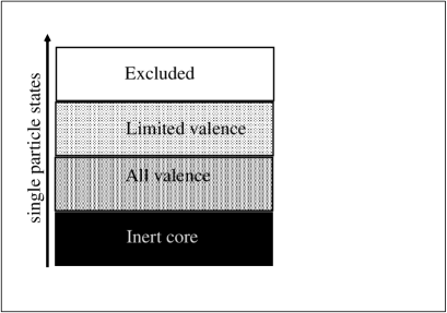
Figure 7: Segregation of single-particle space. ’Inert core’ has all states filled. ‘Excluded’ disallows any occupied states. ‘All valence’ can have states up to the number of valence particles filled, while ‘Limited valence’ can only have fewer states filled (e.g. one, two, three…). See text for discussion.

The first kind of truncation is sometimes called a particle-hole truncation in nuclear physics; in atomic physics (and occasionally in nuclear physics), one uses the notation ‘singles,’ ‘doubles,’ ‘triples,’ etc. To understand this truncation scheme, begin by considering a space of single-particle state, illustrated in Figure 7. The single-particle space can be partitioned into four parts. In the first part, labeled ‘inert core’, the states are all filled and remain filled. In the fourth and final part, labeled ‘excluded,’ no particles are allowed. Both the core and excluded parts of the single-particle space need not be considered explicitly, only implicitly. In some cases there is no core.

More important are the second and third sections, labeled ‘all valence’ and ‘limited valence’, respectively. The total number of particles in these combined sections is fixed at $N_{v}$, and this is the valence or active space.

The difference between the ‘limited valence’ and the ‘all valence’ spaces is that only some maximal number $N_{l}<N_{v}$ of particles are allowed in the ’limited valence’ space. So, for example, suppose we have four valence particles, but only allow at most two particles into the ’limited valence’ space. In this case the ‘all valence’ might contain four, three, or two particles, while the ’limited valence’ space might have zero, one, or two particles. In more standard language, $N_{l}=1$ is called ‘one-particle, one-hole’ or ‘singles’, while $N_{l}=2$ is called ‘two-particle, two-hole’ or ’doubles’, and so on. There are no other restrictions aside from global restrictions on quantum numbers such as parity and $M$.

In nuclear structure physics, where center-of-mass considerations weigh heavily, one sometimes invoke a weighted refinement of this scheme. For all but the lightest systems, one must work in the laboratory frame, that is, the wavefunction is a function of laboratory coordinates, $\Psi=\Psi(r_{1},r_{2},r_{3},\ldots)$. It is only the relative degrees of freedom that are relevant, however, so ideally one would like to be able to factorize this into relative and center-of-mass motion:

$$\Psi(r_{1},r_{2},r_{3},\ldots)=\Psi_{\mathrm{rel}}(\vec{r}_{1}-\vec{r}_{2},\vec{r}_{1}-\vec{r}_{3},\ldots)\times\Psi_{\mathrm{CM}}(\vec{R}_{\mathrm{CM}})$$ (30)

(note that we have only sketched this factorization). In a harmonic oscillator basis and with a translationally invariant interaction, one can achieve this factorization exactly, if the many-body basis is truncated as follows [31, 32, 33]:

$\bullet$ In the non-interacting harmonic oscillator, each single-particle state has an energy $e_{i}=\hbar\Omega(N_{i}+3/2)$. Here $N_{i}$ is the principal quantum number, which is 0 for the $0s$ shell, 1 for the $0p$ shell, 2 for the $1s$-$0d$ shell, and so on. The frequency $\Omega$ of the harmonic oscillator is a parameter but its numerical value plays no role in the basis truncation.

$\bullet$ We can then assign to each many-body state a non-interacting energy $E_{NI}=\sum_{i}e_{i}$, the sum of the individual non-interacting energies of each particle. There will be some minimum $E_{\mathrm{min}}$ and all subsequent non-interacting energies will come in steps of $\hbar\Omega$–in fact for states of the same parity, in steps of $2\hbar\Omega$.

$\bullet$ Now choose some $N_{\mathrm{max}}$, and allow only states with non-interacting energy $E_{NI}\leq E_{\mathrm{min}}+N_{\mathrm{max}}\hbar\Omega$. In practice, restricting states to the same parity means that the ‘normal’ parity will have $E_{NI}=E_{\mathrm{min}}$, $E_{\mathrm{min}}+2\hbar\Omega$, $E_{\mathrm{min}}+4\hbar\Omega,\ldots$, $E_{\mathrm{min}}+N_{\mathrm{max}}\hbar\Omega$, while ‘abnormal’ parity will have $E_{NI}=E_{\mathrm{min}}+\hbar\Omega$, $E_{\mathrm{min}}+3\hbar\Omega,\ldots$, $E_{\mathrm{min}}+N_{\mathrm{max}}\hbar\Omega$.

This is sometimes call the $N\hbar\Omega$ truncation, or simply the energy truncation. It is more complicated than the previous ‘particle-hole’ truncation. We identify with each principal quantum number $N_{i}$ a major shell; for a $4\hbar\Omega$ we can excite four particles each up one shell, one particle up four shells, two particles each up two shells, one particle up one shell and another up three shells, and so on. While complicated, such a truncation allows us to guarantee the center-of-mass wavefunction is a simple Gaussian.

Both truncation schemes can be described by introducing an additional additive quantum number, which we call the weighting $w$ for single-particle states and $W$ for many-body states. Assign to each single-particle state $\phi_{i}$ a non-negative integer $w_{i}$; for example, this might be the principal quantum number for the spherical harmonic oscillator. We assume that states of a given single-particle level (that is, labeled by unique $j_{i},\pi_{i},\alpha_{i}$ but having distinct $m_{i}$) share the same $w_{i}$. The weighting is additive, so that, like $M$, the $W$ for a given many-body state is simply the sum of the $w_{i}$s of the occupied states.

Now, the truncation is simply defined by: allow all states with $W\leq W_{\mathrm{max}}$. (Usually $W_{\mathrm{max}}$ is defined, as in the $N\hbar\Omega$ truncation, relative to some $W_{\mathrm{min}}$.) To regain the simple ‘particle-hole’ truncation, we assign $w=0$ to the ‘all valence’ single-particle states and $w=1$ to the ‘limited valence’ states, and set $W_{\mathrm{max}}=N_{l}$. One can devise, however, more complicated weightings. Because of the inequality and not a strict equality, $W$ is not a ‘good quantum number.’ However we can use nearly the same machinery to implement the inequality as the equality.

This weighted truncation can be and has been implemented into our CI code.

References

- [1] I. Shavitt, Mol. Phys. 94, 3 (1998).
- [2] P.J. Brussard and P.W.M. Glaudemans, Shell-model applications in nuclear spectroscopy (North-Holland Publishing Company, Amsterdam, 1977).
- [3] B. A. Brown and B. H. Wildenthal, Annu. Rev. Nucl. Part. Sci. 38, 29 (1988).
- [4] E. Caurier, G. Martínez-Pinedo, F. Nowacki, A. Poves, and A. P. Zuker, Rev. Mod. Phys. 77, 427 (2005).
- [5] D. B. Cook, Handbook of computational quantum chemistry, (Oxford University Press, Oxford, 1998).
- [6] F. Jensen, Introduction to computational chemistry, 2nd ed. (John Wiley Sons Ltd., West Sussex, 2007).
- [7] P.-O. Löwdin, Phys. Rev. 97, 1474 (1955)
- [8] A. W. Weiss, Phys. Rev. 122, 1826 (1961).
- [9] C.D. Sherrill and H.F. Schaefer III, Adv. Quant. Chem. 34, 143 (1999).
- [10] J. Olsen, B. O. Roos, P. Jørgensen and H. J. A. Jensen, J. Chem. Phys. 89, 2185 (1988).
- [11] J. Olsen, P. Jørgensen, and J. Simons, Chem. Phys. Lett. 169, 463 (1990).
- [12] G. H. Golub and C. F. van Loan, Matrix computations, 3rd ed. (The Johns Hopkins University Press, Baltimore, 1996).
- [13] R. R. Whitehead, A. Watt, B. J. Cole, and I. Morrison, Adv. Nucl. Phys. 9, 123 (1977).
- [14] R R Whitehead and A Watt, J. Phys. G 4 (1978) 835; R. R. Whitehead, in Theory and applications of moment methods in many-fermion systems, edited by B.J. Dalton, S.M. Grimes, J.P. Vary, and S.A. Williams, p. 235. (Plenum Press, New York, 1980).
- [15] B. A. Brown, A. Etchegoyen, and W. D. M. Rae, computer code OXBASH, the Oxford University-Buenos Aires-MSU shell model code, Michigan State University Cyclotron Laboratory Report No. 524, 1985.
- [16] http://www.garsington.eclipse.co.uk/
- [17] J.P. Vary, The Many-Fermion Dynamics Shell-Model Code, Iowa State University (1992) (unpublished); J.P. Vary and D.C. Zheng, ibid., (1994) (unpublished); P. Sternberg, E. Ng, C. Yang, P. Maris, J.P. Vary, M. Sosonkina, H. Viet Le, “Accelerating configuration interaction calculations for nuclear strucure,” in the Proceedings of the 2008 ACM/IEEE Conference on Supercomputing, IEEE Press, Piscataway, NJ, doi.acm.org/10.1145/1413370.1413386.
- [18] E. Caurier and F. Nowacki, Acta Phys. Pol. B 30 (1999) 705.
- [19] E. Caurier et al., Phys. Rev. C 59 (1999) 2033.
- [20] J. Toivanen, computer code EICODE, JYFL, Finland, 2004.
- [21] J. Toivanen, arXiv:nucl-th/0610028.
- [22] F. Andreozzi and A. Porino, J. Phys. G 27 (2001) 845.
- [23] T. Papenbrock and D. J. Dean, Phys. Rev. C 67 (2003) 051303.
- [24] T. Papenbrock, A. Juodagalvis, and D. J. Dean, Phys. Rev. C 69 (2004) 024312.
- [25] T. Papenbrock and D. J. Dean, J. Phys. G 31 (2005) S1377.
- [26] I. Lindgren and J. Morrison, Atomic many-body theory, 2nd. ed. (Springer-Verlag, Berlin, 1985).
- [27] E. R. Davidson, Comput. Phys. 7, 519 (1993).
- [28] M. L. Leininger, C. D. Sherrill, W. D. Allen, and H. F. Schaefer III, J. Comp. Chem. 22, 1574 (2001).
- [29] J. P. Vary and P. Maris, private communication.
- [30] J.-Q. Chen, Group representation theory for physicists (World Scientific, Singapore, 1989).
- [31] F. Palumbo, Nucl. Phys. A 99, 100 (1967).
- [32] F. Palumbo and D. Prosperi, Nucl. Phys. A 115, 296 (1968).
- [33] D. H. Gloeckner and R. D. Lawson, Phys. Lett. B 53, 313 (1974).