A new technique for the determination of the initial mass function in unresolved stellar populations

Abstract

We present a new technique for the determination of the low-mass slope ($\alpha_{1}$; $M_{*}<0.5M_{\odot}$) of the present day stellar mass function (PDMF) using the pixel space fitting of integrated light spectra. It can be used to constrain the initial mass function (IMF) of stellar systems with relaxation timescales exceeding the Hubble time and testing the IMF universality hypothesis. We provide two versions of the technique: (1) a fully unconstrained determination of the age, metallicity, and $\alpha_{1}$ and (2) a constrained fitting by imposing the externally determined mass-to-light ratio of the stellar population. We have tested our approach by Monte-Carlo simulations using mock spectra and conclude that: (a) age, metallicity and $\alpha_{1}$ can be precisely determined by applying the unconstrained version of the code to high signal-to-noise datasets (S/N=100, $R=7000$ yield $\Delta\alpha_{1}\approx 0.1$); (b) the $M/L$ constraint significantly improves the precision and reduces the degeneracies, however its systematic errors will cause biased $\alpha_{1}$ estimates; (c) standard Lick indices cannot constrain the PDMF because they miss most of the mass function sensitive spectral features; (d) the $\alpha_{1}$ determination remains unaffected by the high-mass IMF shape ($\alpha_{3}$; $M_{*}\geq 1M_{\odot}$) variation for stellar systems older than 8 Gyr, while the intermediate-mass IMF slope ($\alpha_{2}$; $0.5\leq M_{*}<1M_{\odot}$) may introduce biases into the best-fitting $\alpha_{1}$ values if it is different from the canonical value $\alpha_{2}=2.3$. We analysed observed intermediate resolution spectra of ultracompact dwarf galaxies with our technique and demonstrated its applicability to real data.

1 Introduction

The stellar IMF is one of the most important intrinsic properties of the star formation process. Its origin still remains unclear. Historically, it was thought to be a unimodal power law function $dN/dM\propto M^{-(\alpha-1)},\alpha=2.35$ (Salpeter, 1955). The current working hypothesis (Kroupa, 2002) of the IMF universality suggests that its shape does not vary among different star forming regions and can be represented as a bimodal power law with different low- and high-mass slopes ($\alpha_{1}=1.3$ for $M<0.5\,M_{\odot}$ and $\alpha_{2}=2.3$ at larger masses). Other possibilities include variations of uni- or multi-modal power laws (e.g. Miller & Scalo, 1979) or a lognormal function (Chabrier, 2003). The IMF shape has a direct impact on galaxy evolution because it defines the number of Wolf–Rayet stars and supernovae and therefore the amount of star formation feedback. The low-mass IMF slope has strong influence on stellar mass-to-light ratios because of high $M/L$ values of dwarf late type stars.

Classical IMF determination techniques (see Kroupa (2002) for a review) use direct star counts in open clusters and Hii associations. However, they are affected by various phenomena such as dynamical evolution of star clusters, variable and often strong dust extinction in star forming regions, as well as by the low number statistics. In this light, compact stellar systems (CSS), that is globular clusters (GC) and ultracompact dwarf galaxies (UCD, Drinkwater et al., 2003) which are orders of magnitude more massive, free of the interstellar medium and populated by old stars present a unique laboratory to study the IMF.

CSSs observed today might have experienced dynamical evolution effects on their stellar mass functions, i.e. the observed PDMF may differ from the IMF. It is known (Spitzer, 1987; Baumgardt & Makino, 2003; Khalisi et al., 2007; Kruijssen & Mieske, 2009) that in globular clusters the dynamical evolution causes mass segregation, i.e. massive stars move towards the centre while low-mass stars migrate to the cluster outskirts, where they are tidally stripped during the passages close to the centre of a host galaxy or through its disc. This creates a deficit of low-mass stars in a cluster, changing the shape of its integrated stellar mass function. The characteristic timescale of this process is related to the dynamical relaxation time, which can be estimated for a CSS (Mieske et al., 2008) as ${t_{\rm rel}}=\frac{0.234}{\log{M_{\rm dyn}}}\sqrt{\frac{M_{\rm dyn}{r_{e}^{3}}}{0.0045}}$ Myr, where ${M_{\rm dyn}}$ is in $M_{\odot}$ and the effective radius ${r_{e}}$ is in pc. Sufficiently massive GCs and UCDs have long relaxation timescales (a few Gyrs to many $t_{\rm Hub}$) and therefore we can neglect the dynamical evolution effects in those systems. Hence, the PDMF there becomes a good approximation of the IMF for low-mass stars which have not yet finished their evolution.

One has to keep in mind that the mass segregation is not the only process which may result in the low-mass stars deficiency in CSSs. It can also be caused by the residual-gas expulsion from initially mass segregated star clusters, as it was shown for galactic GCs (Marks et al., 2008) and UCDs (Dabringhausen et al., 2010). However, the dynamical analysis of Fornax cluster UCDs does not show any signs of the lack of low-mass stars in these relatively massive systems (Mieske et al., 2008; Chilingarian et al., 2011). There is also a strong relationship between the low-mass IMF slope and the concentration in GCs (De Marchi et al., 2007). It turns out to be possible to estimate the phase of the low-mass star loss process from observations and therefore to make a conclusion about the equivalence of PDMF and IMF for every particular CSS.

In this paper we describe a new technique of deriving the low-mass IMF slope by using the pixel fitting of intermediate- and high-resolution spectra of stellar systems integrated along the line of sight. This approach is inspired by the results of Chilingarian et al. (2008, 2011) where the stellar masses derived using the Salpeter (1955) IMF turned to exceed the dynamical mass estimates resulting in unphysical negative dark matter contents.

2 New method: simulations and applications

We present two versions of the technique to derive the low-mass slope of the stellar IMF from integrated light spectra using full spectral fitting developed as an extension of the nbursts package (Chilingarian et al., 2007a, b).

nbursts is an approach to determine the parametrized line-of-sight velocity distribution (LOSVD) and star formation history (SFH) of unresolved stellar populations by means of the full spectral fitting in the pixel space. Previously the nbursts technique was mostly used with simple stellar population (SSP) models characterized by only two parameters, age and metallicity of the instantaneous starburst event computed for a pre-defined IMF shape. In this study, we added an extra dimension to the grid of SSP models by varying the low-mass end slope $\alpha_{1}$ of the Kroupa canonical IMF (Kroupa, 2002) leaving the slope above $0.5M_{\odot}$ fixed ($\alpha_{2}=2.3$). Hence, $\alpha_{1}$ becomes an additional free parameter returned by the modified fitting procedure. We computed stellar population models for “non-standard” $\alpha_{1}$ values using both, high and low resolution stellar atmosphere grids supplied with the pegase.hr evolutionary synthesis code (Le Borgne et al., 2004), the empirical high resolution elodie.3.1 stellar library (Prugniel et al., 2007) and the low resolution BaSeL theoretical atmospheres (Lejeune et al., 1997) used in the original pegase.2 package (Fioc & Rocca-Volmerange, 1997). The full spectral fitting is performed with high-resolution models while the mass-to-light ratios of stellar populations in broad band filters are estimated using the low-resolution grid. We used standard pegase.hr settings for all other parameters: 5 per cent of close binary systems, low and high cut-off stellar masses of 0.1 and 120 $M_{\odot}$ correspondingly.

In the first version of our new approach an observed spectrum is fitted against an optimal template represented by a linear combination of SSPs each of them characterised by the age, metallicity and the low-mass IMF slope $\alpha_{1}$, determined in the same minimization loop, using the 3-dimensional cubic spline interpolation on the pre-computed grid of high-resolution SSP models.

In this paper we deal with observed spectra of CSSs which can be well represented by single component SSP models, however the code provides a possibility of fitting multiple component stellar populations. The model grid has 25 nodes in age (10 Myr to 20 Gyr), 10 nodes in metallicity ([Fe/H] from -2.5 to 1.0 dex) and 10 nodes in the low-mass IMF slope (0.4 to 3.1 with a step of 0.3). During the fitting procedure, the models are broadened using the Gauss-Hermite parametrization (van der Marel & Franx, 1993) of the LOSVD which is penalized toward purely Gaussian solution as proposed by Cappellari & Emsellem (2004). In this paper we consider only purely Gaussian LOSVDs.

The ${{\chi}^{2}}$ value (without penalization) is computed as follows:

$${{\chi}^{2}}=\sum\limits_{{N_{\lambda}}}\frac{\bigl{(}{F_{i}}-{P_{1p}}({T_{i}}(t,Z,\alpha_{1})\otimes\mathcal{L}(v,\sigma,{h_{3}},{h_{4}})+{P_{2q}})\bigr{)}^{2}}{{\Delta}{{F_{i}}^{2}}}$$ (1)

where ${F_{i}}$ and ${\Delta}{{F_{i}}}$ are observed flux and its uncertainty; $\mathcal{L}$ is LOSVD used as a convolution kernel for ${T_{i}}(t,Z,\alpha_{1})$, the flux from a synthetic spectrum, represented by a linear combination of SSP models characterised by their ages $t$, metallicities $Z$, and low-mass IMF slopes $\alpha_{1}$, and convolved according to the line-spread function of the spectrograph; ${P_{1p}}$ and ${P_{2q}}$ are multiplicative and additive Legendre polynomials of orders $p$ and $q$ for correcting the continuum; $v$, $\sigma$, ${h_{3}}$ and ${h_{4}}$ are radial velocity, velocity dispersion and Gauss-Hermite coefficients of the LOSVD respectively.

The ${\chi^{2}}$ minimization is performed using the constrained non-linear Levenberg–Marquardt minimization implemented in the mpfit IDL package (by C. Markwardt, NASA). Since it requires the second derivatives to be continuous, we use a three-dimensional spline interpolation of the SSP grid to evaluate a model for a given set of ($t$, [Fe/H], $\alpha_{1}$). In this fashion, the values of $t$, [Fe/H], and $\alpha_{1}$ are returned by the minimization procedure in the same loop along with the parameters of the continua.

The second version of our technique is mathematically identical to the pure nbursts technique but the specific grid of input SSP models is constructed and supplied for every observed spectrum. Here we assume that the object being studied contains no dark matter. This assumption is probably true for GCs and UCDs. In this case, the dynamical mass-to-light ratio $(M/L)_{\rm{dyn}}$ equals to the stellar mass-to-light ratio $(M/L)_{*}$. For a number of compact stellar systems, the $(M/L)_{\rm{dyn}}$ values were determined from the analysis of their internal structure and observed velocity dispersion profiles and are available in the literature. On the other hand, we derive the $(M/L)_{*}$ values from low-resolution stellar population models for every set of ($t$, [Fe/H], $\alpha_{1}$) and for every given $t$ and [Fe/H] in the old stellar population regime this function is monotonic. Hence, if we know $(M/L)_{\rm{dyn}}$ and impose the zero dark matter constraint, for every point on the ($t$, [Fe/H]) plane we can find the value of $\alpha_{1}$ such as $(M/L)_{*}$ in that point of the parameter space equals to $(M/L)_{\rm{dyn}}$. Thus, we can compute a grid of SSP models in the age–metallicity space varying the low-mass IMF slope so that the $(M/L)_{*}$ values are constant all over the grid and equal to the “external” $(M/L)_{\rm{dyn}}$. Along with this grid, we will also map the behaviour of $\alpha_{1}$ as a function of $t$ and [Fe/H]. Then, if we feed this SSP grid to the standard nbursts full spectral fitting procedure and determine the pair of best-fitting values of age and metallicity, we will automatically get the $\alpha_{1}$ value corresponding to this best-fitting solution which will measure the low-mass PDMF slope of the stellar population being studied.

It may happen that in order to reach the imposed value of $(M/L)$ the low-mass IMF slope has to be outside our model grid ($0.4<\alpha_{1}<3.1$). In this case, we take the model corresponding to the nearest limiting $\alpha_{1}$ value (maximal or minimal).

In some cases, e.g. high-resolution spectra of extragalactic GCs or UCDs where the internal velocity dispersion can be measured from a spectrum itself and where it uniquely defines $(M/L)_{\rm{dyn}}$, it is possible to modify the minimization procedure and close the loop so that no external $(M/L)$ value needs to be supplied. However, in this case the procedure becomes very complex and we do not consider this approach in this paper. As we demonstrate from simulations, velocity dispersion does not exhibit any degeneracies with age and $\alpha_{1}$, therefore if $\sigma$ is determined independently, it should not affect the final $\alpha_{1}$ estimate.

2.1 Full spectral fitting of mock data

We performed Monte-Carlo simulations in order to study the precision, stability, and possible biases of the proposed technique for the determination of the low-mass IMF slope. We generated mock datasets (10 to 1000 noise realisations for every combination of input parameters) for the signal-to-noise ratios of 25, 50, and 100, and the spectral resolution values $R=4000\dots 10000$. Then we fitted them using both versions of our technique.

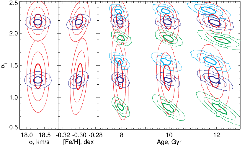
Figure 1: Results of the full spectral fitting of mock spectra. Red and blue contours correspond to the first (all free parameters) and the second (constrained M/L) versions of the technique. Cyan and green contours demonstrate how biased values of $M/L$ ratios affect the results in the constrained version of the technique. Contours correspond to the 1-, 2- and 3-$\sigma$ levels.

In Fig. 1 we present the results of the full spectral fitting of 1800 mock spectra (300 noise realisations for the ages $t$=8, 10 and 12 Gyr; $Z=-0.3$ dex; $\alpha_{1}=$1.3 and 2.2, i.e. close to Kroupa and Salpeter IMFs) for the spectral resolution $R=7000$ and the signal-to-noise ratio S/N=100 in the wavelength range 3900$\dots$6800 Å. The results are presented in a way showing the degeneracies between derived stellar population parameters and the $\alpha_{1}$ IMF slopes. The results of the simulations made using metal-poor stellar populations ([Fe/H]=$-1.0$ dex) look very similar except the $\sim$30 per cent higher uncertainties.

Here we see that even the first version of the technique is able to recover the $\alpha_{1}$ values with the uncertainty of about 0.1–0.2. When we impose the $M/L$ ratio, the precision significantly improves and the uncertainties of $\alpha_{1}$ become better than 0.1. We see the strong age–$\alpha_{1}$ degeneracy because the higher mass fraction of low-mass stars in older populations may compensate the lower derived values of $\alpha_{1}$. The accuracy of about 0.06 well compares to the best available IMF determination for Galactic open clusters Pleiades ($\Delta\alpha_{1}$=0.15) and M35 ($\Delta\alpha_{1}$=0.12) presented in Kroupa (2002).

In order to test the sensitivity of the second version of our technique to the biased input $M/L$ values, we performed the simulations increasing and decreasing the $M/L$ expected from the stellar population models by 10 per cent. The results are shown in Fig. 1 by green ($0.9\cdot M/L$) and cyan ($1.1\cdot M/L$) contours. It demonstrates how $M/L$ systematic errors translate into $\alpha_{1}$ biases. One has to keep in mind that usually the dynamical mass of a real stellar systems is known with the precision worse than 10 per cent.

2.2 The analysis of the distribution of the IMF sensitive information

For the practical usage of our technique and future impovements of the observational strategy to study the IMF in real stellar systems, one needs to know which spectral features have the highest sensitivity to the IMF shape. In order to identify them, we analysed the distribution of the $\alpha_{1}$-sensitive information in 20Å-wide bins in the optical spectral domain for metal-rich and metal-poor stellar population in a similar fashion to that proposed in Chilingarian (2009) for the analysis of age and metallicity sensitivity. For our test (see Fig. 2 we chose two high resolution ($R=10000$) pegase.hr SSP models in the wavelength range 3920$\dots$6700 Å  with the age $t=10$ Gyr and $\alpha_{1}$=1.3 having metallicities [Fe/H]=$-1.0$ and $-0.3$ dex. Then, we convolved them with Gaussian kernels corresponding to the internal velocity dispersions of 10 km s^-1 and thus obtained two model spectra or “reference SSPs”. Then for every of them we varied the $\alpha_{1}$ value by 0.1. Later, we fitted these models against their “reference SSPs” using the pPXF procedure (Cappellari & Emsellem, 2004) with the 10th order multiplicative polynomial continuum. The total amount of “information” equals to the sum of partial derivatives of ${{\chi}^{2}}$ as a function of $\alpha_{1}$ over all pixels normalised to 100 per cent. The Nai D line region shown in yellow in Fig. 2 is excluded from consideration because it is a feature in stellar spectra heavily affected by the interstellar absorption line and therefore cannot be reliably modelled in the evolutionary synthesis.

We see that the distributions are very similar for metal-rich and metal-poor populations (red and blue histograms respectively). An exception is the H$\alpha$ line (6563 Å) which contains considerable amount of the information for metal-poor populations and is less significant at higher metallicities. Most of the IMF-sensitive spectral regions are those containing numerous but relatively faint absorption lines sensitive to the surface gravity in the atmospheres of late type (GKM) stars. These lines are concentrated on both sides of H$\beta$ (4760–4800Å and 4900–4960Å) and between 5400Å and 6400Å with the most sensitive part around 6100Å associated with Cai, Vi, Coi, Nii, and Tii absorption lines. Worth mentioning that when varying $\log g$, the Cai lines change in the opposite direction compared to all other elements from the list above. Details will be given in a separate paper.

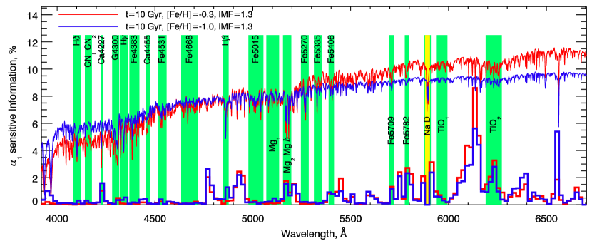
Figure 2: The distribution of $\alpha_{1}$-sensitive information along the wavelength in 20 Å-wide bins in the high-resolution (R=7000) spectra of metal-rich (red, [Fe/H]=-0.3 dex) and metal-poor (blue, [Fe/H]=-1.0 dex) stellar populations. The distributions are normalised to the unity (100 per cent). The stellar population spectra are shown above. The Nai D region shown in yellow is excluded from consideration (see the text). Green areas denote the Lick index definitions. We clearly see that apart from a few exceptions, the IMF-sensitive information is not associated with Lick indices (see the text).

2.3 Effects of the high-mass IMF shape on the $\alpha_{1}$ determination

In this study we use the Kroupa canonical IMF (Kroupa, 2002) by varying the low-mass end slope $\alpha_{1}$ and leaving the high-mass slope fixed ($\alpha_{2}=2.3$). Recently, Marks et al. (2012) have demonstrated that stellar systems which underwent high star formation volume densities at a parsec scale require the introduction of $\alpha_{3}$ for massive stars ($>1M_{\odot}$). Using Monte-Carlo simulations we have checked how changes of $\alpha_{3}$ influence the fitting results for a “standard” bi-modal canonical IMF. We generated 4500 spectra (300 noise realisations for the ages $t$=4, 6, 8, 10 and 12 Gyr; $\alpha_{3}$=1.7, 2.0 and 2.6, $\alpha_{1}$=1.3, $[$Fe/H$]=-1.0$ dex). Then we fitted them using the first version of our technique with a model grid having $\alpha_{3}=2.3$. The results of this fitting are presented in Fig. 3 as data points connected by solid lines.

Here we clearly see that the $\alpha_{1}$ determination remains unaffected by $\alpha_{3}$ values for stellar systems older than 8 Gyr. It is trivially explained by the fact that the lifetime of massive stars ($>1M_{\odot}$) is shorter than 8 Gyr therefore they do not contribute to the integrated light of a stellar system. The conclusion from this experiment is that any stellar system of the age of 8 Gyr or older can be analysed with our standard set of the SSP models with the fixed value of $\alpha_{3}=2.3$ when using the first version of our IMF determination technique.

We performed similar analysis in order to test how the best-fitting $\alpha_{1}$ values are affected by the variations of $\alpha_{2}$. We generated 3000 mock spectra (300 noise realisations for the ages $t$=4, 6, 8, 10 and 12 Gyr; $\alpha_{2}$=2.0 and 2.6, $\alpha_{1}$=1.3, metallicity $Z=-1.0$ dex). Then we fitted them in a similar fashion to the $\alpha_{3}$ test. These results are also shown in Fig. 3 as data points connected by dash dot lines.

We see that $\alpha_{2}$ variations introduce significant biases into the best-fitting $\alpha_{1}$ values. The bias is larger for younger populations ($\alpha_{1}$=2.0 instead of 1.3 for 4 Gyr) than for older populations ($\alpha_{1}$=1.7 instead of 1.3 for 12 Gyr). This fact is also easy to explain by the theory of stellar evolution: for older stellar populations all massive stars have already evolved into the remnants and the contribution of stars with masses $M>0.5M_{\odot}$ decreases as the age increases. The lower $\alpha_{2}$ values correspond to the excess of these stars compared to the canonical IMF shape and when we fit such a spectrum with the models computed for $\alpha_{2}=2.3$, it requires shallower low-mass end slope $\alpha_{1}$ to partially compensate the lack of more massive stars which were present in the model because of lower $\alpha_{2}$.

However, we stress that according to recent studies there is no evidence for $\alpha_{2}$ to vary: “The IMF of massive stars is well described by a Salpeter/Massey slope, $\alpha_{2}$ = 2.3, independent of environment as deduced from resolved stellar populations in the Local Group of galaxies. Unresolved multiple stars do not significantly affect the massive-star power-law index” (Kroupa et al., 2011).

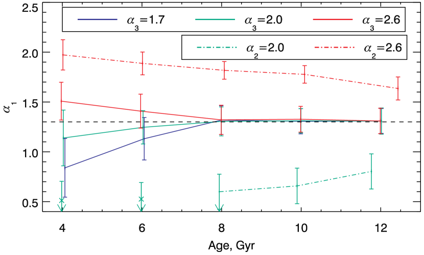
Figure 3: The $\alpha_{1}$ determination biases introduced by the variations of $\alpha_{2}$ and $\alpha_{3}$. For every set of parameters, error bars show the standard deviation of the best-fitting $\alpha_{1}$ calculated from 300 noise realisations in every point. Solid and dash dot lines are for the fitting results when varying $\alpha_{3}$ and $\alpha_{2}$ respectively. Arrows indicate that the lower limit of the model grid ($\alpha_{1}=0.4$) was reached for some mock spectra.

2.4 Full spectral fitting of real data

We applied our technique to observed spectra having different signal-to-noise ratios, spectral resolutions and wavelength coverages. We used three publicly available datasets for compact stellar systems: (1) intermediate resolution (R=1300) Galactic GC spectra from Schiavon et al. (2005) obtained with the R-C spectrograph at the 4 m Blanco telescope at CTIO in the wavelength range 3900$<\lambda<$6500 Å; (2) high-resolution (R=17000) intermediate signal-to-noise spectra of UCDs in the Fornax cluster obtained with FLAMES/Giraffe at ESO VLT in the HR9 setup covering a narrow wavelength interval, 5120$<\lambda<$5450Å  (Mieske et al., 2008; Chilingarian et al., 2011) downgraded to R=10000, and (3) intermediate resolution (R=1500–2000) high signal-to-noise ratio spectra (3900$<\lambda<$6800 Å) of Fornax and Virgo cluster UCDs obtained with Gemini GMOS-N/GMOS-S (Francis et al., 2012).

The dynamical $M/L$ measurements for some of Schiavon et al. (2005) spectra were available from Dubath et al. (1997) and Lane et al. (2010). However, none of the clusters had $t_{\mbox{rel}}>4$ Gyr, and those spectra were integrated and extracted only in the cluster core region. In addition, classical long-slit spectra of GCs used for the dynamical analysis and consequently our MF analysis suffer from systematic uncertainties caused by the limited number of individual stars falling into the slit (see discussion in Dubath et al., 1997). Another problem is that the nuclear regions will have higher weights over peripheral parts because the cluster light fraction falling into the slit decreases as $R^{-1}$. Therefore, we could not obtain any reliable estimates of $\alpha_{1}$ values in these objects but only use them to evaluate statistical errors of the techniques for spectra of such a type. The statistical uncertainties of the first version of our technique turned to be about $\Delta\alpha_{1}\approx$0.3–0.5. Fixing the M/L values reduced them down to 0.15.

Spectra of extragalactic clusters and UCDs have a number of advantages over Galactic GC spectra although they are more difficult to obtain because the targets are much fainter. The main advantage is that these spectra will be very close to the integrated spectra because at the distance of Virgo and Fornax CSSs usually stay unresolved from the ground. Therefore, there will be no systematic errors connected to the low number statistics of stars on the slit, and also there will be no $R^{-1}$ weighting of peripheral parts. Another advantage is that in rich environments such as Fornax and Virgo, the number of GCs is so high that they populate very well even the brighter end of the luminosity function, therefore it becomes easy to find objects with $t_{\rm rel}\geq t_{\rm Hub}$ which did not undergo the dynamical evolution and therefore are suitable for the determination of IMF and not only the PDMF.

Our experiments with the high-resolution FLAMES/Giraffe spectra of Fornax cluster GC/UCDs demonstrate that those data can be used for the PDMF determination only if the dynamical $M/L$ values are known from the analysis of their internal dynamics and structural properties. Then the statistical uncertainties of the $M/L$ constrained fitting stay in the range of 0.05$\dots$0.1 depending on the S/N ratio and the overall errors are systematic and fully imposed by the $M/L$ uncertainties. However, very short wavelength range not including any strong IMF sensitive features makes the $\alpha_{1}$ determination impossible for the first unconstrained version of our technique bringing the statistical error to $\Delta\alpha_{1}=$0.8 even for the brightest object, UCD 3 (F 19 in Chilingarian et al., 2011).

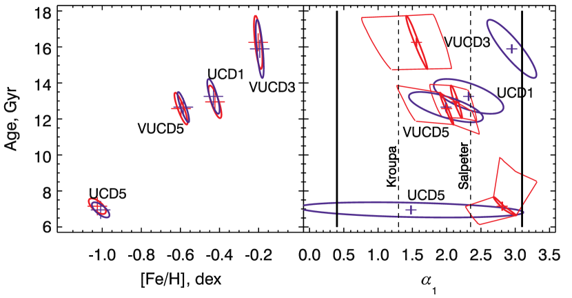
Figure 4: Determination of the low-mass IMF slope using both versions of our technique for four UCDs: UCD 1 and UCD 5 from the Fornax cluster; VUCD 3 and VUCD 5 from the Virgo cluster. Blue and red crosses and ellipses denote the best fitting values and their 1-$\sigma$ statistical uncertainties computed from the covariance matrix for the unconstrained and $M/L$ constrained versions of our technique correspondingly. Red boxes demonstrate the range of systematic errors for the constrained fitting corresponding to 1-$\sigma$ uncertainties of the adopted $M/L$ ratios. Black lines on the lower panel show the limits of our grid of SSP models.

Analysis of high S/N integrated spectra for Virgo/Fornax UCDs obtained with Gemini GMOS-N and GMOS-S spectrographs in a broad wavelength range demonstrates a reasonably good agreement between the two versions of our technique (see Fig 4). We used published dynamical $M/L$ ratios for two Virgo cluster UCDs (VUCD 3 and VUCD 5, Evstigneeva et al., 2007) and two Fornax cluster UCDs (UCD 1 and UCD 5, Chilingarian et al., 2008). The adopted $(M/L)_{V,\mbox{dyn}}$ values in the Solar units are: $5.4\pm 0.9$, $4.1\pm 0.8$, $5.0\pm 0.6$, and $3.4\pm 0.9$ for VUCD 3, VUCD 5, UCD 1, and UCD 5 correspondingly. For UCD 1 and VUCD 5 both, fully unconstrained fitting and the $M/L$-imposed version of the technique agree well within the statistical uncertainties of the unconstrained fitting. For UCD 5 having low metallicity and therefore much weaker absorption lines, the unconstrained fitting results in very large uncertainties while the adopted $(M/L)_{V}$ value puts it close to the edge of the model grid on the MF slope (2.8). For VUCD 3 the situation is the opposite, the unconstrained fitting yields $\alpha_{1}\approx 2.9$, however one has to keep in mind that this object has extremely high value of the [$\alpha$/Fe] chemical abundance ratio (Francis et al., 2012) resulting in the significant template mismatch, therefore the unconstrained measurements may get biased. At present, we do not have models required to study the biases which may be introduced to the MF measurements from integrated light spectra by significantly non-solar abundance ratios.

3 Discussion and Summary

We presented a novel technique for the determination of the low-mass end slope of the PDMF of unresolved stellar populations using pixel fitting of spectra integrated along the line of sight. In stellar systems with long dynamical relaxation timescales such as massive GCs, UCDs and galaxies, where one can neglect the effects of the dynamical evolution, the PDMF is identical to the IMF at low masses. Our technique is available in two versions having different applications: (a) fully unconstrained determination of age, metallicity and the low-end PDMF slope $\alpha_{1}$ which can be used to analyse high signal-to-noise spectra of CSSs and normal galaxies given that the wavelength coverage includes IMF sensitive features; (b) constrained determination of the same parameters by imposing the external value of the $M/L$ ratio which can be, for example obtained from the dynamical modelling and therefore assuming the zero dark matter content in a stellar system being studied.

We used Monte-Carlo simulations with mock spectra to test both approaches and conclude that: (1) age, metallicity, and IMF can be precisely determined in the first unconstrained version of the code for high signal-to-noise datasets (e.g. S/N=100, R=7000 give the uncertainty of $\alpha_{1}$ of about 0.1–0.2); (2) adding the $M/L$ information significantly improves the precision and reduces the degeneracies, however systematic errors in the imposed $M/L$ ratio will translate into offsets in $\alpha_{1}$.

We performed the analysis of the IMF-sensitive information distribution across the optical spectral domain. One can clearly see in Fig. 2 that apart from a few exceptions, IMF sensitive information is not associated with prominent absorption line features (and line strength indices corresponding to them, e.g. Lick indices, see Worthey, 1994) where a significant fraction of age- and metallicity-sensitive information is contained. The exceptions are: the Cai feature ($\lambda=4227$ Å) and the Mg$b$ triplet ($\lambda\approx 5172$ Å). However, these two indices are very sensitive to the metallicity and the [$\alpha$/Fe] abundance ratios and therefore can hardly be used to constrain the IMF. Another IMF sensitive Lick index is Fe5782 which is known to be difficult to measure and calibrate. The only strong IMF feature left is the TiO₂ index including about 7 per cent of the total IMF-sensitive information. Hence, “standard” absorption line strength indicators cannot be used to determine $\alpha_{1}$.

According to the recent studies (Marks et al., 2012), the stellar IMF at high masses ($>1M_{\odot}$) appears to depend on the star-formation rate density on a parsec scale and even becomes top-heavy when it surpasses 0.1$M_{\odot}$ / (${{\rm yr}\cdot{\rm pc}}^{3}$). It may become increasingly bottom-heavy at high metallicity. The increased number of compact stellar remnants such as neutron stars and black holes for a top-heavy IMF will elevate the $M/L$ values (Dabringhausen et al., 2009) and mimic the dark matter in CSSs. Conversely, for a top-light IMF the $M/L$ will be lower then for the canonical Kroupa IMF. This will become a caveat for the second ($M/L$ constrained) version of our technique because the $M/L$ ratios computed from the stellar population models based on the Kroupa canonical IMF will be incorrect. We quantified this effect by comparing the pegase.2 predictions of stellar $M/L$ ratios for stellar populations having different $\alpha_{1}$, $\alpha_{3}$, and ages. As expected, the $\alpha_{3}$-induced $M/L$ variations are the most important for bottom-light populations ($\alpha_{1}<1$) because of the higher relative mass fraction of stellar remnants. However, the overall effect of the $\alpha_{3}$ variations on $M/L$ ratios is lower than that of $\alpha_{1}$ for the same amount of the IMF slope change. For instance, going from $\alpha_{3}=2.3$ to $\alpha_{3}=1.7$ changes the $V$ band $M/L$ ratio by 11 (for $\alpha_{1}=3.1$) to 26 per cent (for $\alpha_{1}=0.4$) for ages exceeding 10 Gyr. For 8 Gyr the effect is even 2 per cent smaller. The top-light IMF ($\alpha_{3}=2.6$) lowers the $M/L$ by as little as 1 to 6 per cent for ages above 8 Gyr.

At the same time, the unconstrained version of our fitting technique will provide correct estimates of the low-mass IMF slope if applied to older stellar populations ($t>8$ Gyr) where massive stars affecting the variable high-end IMF slope have already evolved into stellar remnants (see section 2.3). It also can be applied to the data for galaxies because the assumed dark matter content does not have to be zero. The unconstrained version can be applied to check whether the IMF is bottom heavy in massive elliptical galaxies where low-mass stars might have efficiently formed in cooling flows (Kroupa & Gilmore, 1994). However, we have to keep in mind that the difference between SSPs and real star formation histories of galaxies as well as significantly non-solar element abundance ratios may introduce some biases.

We applied our technique to observed spectra of CSSs and demonstrated that even for low resolution datasets ($R=1500$) with high S/N-ratios the IMF slope can be precisely determined even using the unconstrained fitting of $\alpha_{1},t,[$Fe/H$]$. The $M/L$ constrained approach provides even higher precision and agrees well with the unconstrained version for objects without peculiarities in stellar populations and chemical abundances.

High spectral resolution will improve the precision only if IMF-sensitive spectral features are covered. Extragalactic GC systems where structural parameters of clusters are available from the Hubble Space Telescope data will have advantage over the Galactic GCs because the integrated velocity dispersion measurements of such systems are much easier to obtain for large samples of targets using multi-object spectroscopy.

We conclude that by applying our technique to high-quality optical observations of CSSs we are able to reach better precision of the IMF determination than that made with direct star counts in nearby open clusters and check the IMF universality hypothesis.

References

- Baumgardt & Makino (2003) Baumgardt, H. & Makino, J. 2003, MNRAS, 340, 227
- Cappellari & Emsellem (2004) Cappellari, M. & Emsellem, E. 2004, PASP, 116, 138
- Chabrier (2003) Chabrier, G. 2003, PASP, 115, 763
- Chilingarian et al. (2007a) Chilingarian, I., Prugniel, P., Sil’chenko, O., & Koleva, M. 2007a, in IAU Symposium, Vol. 241, Stellar Populations as Building Blocks of Galaxies, ed. A. Vazdekis & R. R. Peletier (Cambridge, UK: Cambridge University Press), 175–176, arXiv:0709.3047
- Chilingarian (2009) Chilingarian, I. V. 2009, MNRAS, 394, 1229
- Chilingarian et al. (2008) Chilingarian, I. V., Cayatte, V., & Bergond, G. 2008, MNRAS, 390, 906
- Chilingarian et al. (2011) Chilingarian, I. V., Mieske, S., Hilker, M., & Infante, L. 2011, MNRAS, 412, 1627
- Chilingarian et al. (2007b) Chilingarian, I. V., Prugniel, P., Sil’chenko, O. K., & Afanasiev, V. L. 2007b, MNRAS, 376, 1033
- Dabringhausen et al. (2010) Dabringhausen, J., Fellhauer, M., & Kroupa, P. 2010, MNRAS, 403, 1054
- Dabringhausen et al. (2009) Dabringhausen, J., Kroupa, P., & Baumgardt, H. 2009, MNRAS, 394, 1529
- De Marchi et al. (2007) De Marchi, G., Paresce, F., & Pulone, L. 2007, ApJ, 656, L65
- Drinkwater et al. (2003) Drinkwater, M. J., Gregg, M. D., Hilker, M., Bekki, K., Couch, W. J., Ferguson, H. C., Jones, J. B., & Phillipps, S. 2003, Nature, 423, 519
- Dubath et al. (1997) Dubath, P., Meylan, G., & Mayor, M. 1997, A&A, 324, 505
- Evstigneeva et al. (2007) Evstigneeva, E. A., Drinkwater, M. J., Jurek, R., Firth, P., Jones, J. B., Gregg, M. D., & Phillipps, S. 2007, MNRAS, 378, 1036
- Fioc & Rocca-Volmerange (1997) Fioc, M. & Rocca-Volmerange, B. 1997, A&A, 326, 950
- Francis et al. (2012) Francis, K. J., Drinkwater, M. J., Chilingarian, I. V., Bolt, A. M., & Firth, P. 2012, MNRAS, 425, 325
- Khalisi et al. (2007) Khalisi, E., Amaro-Seoane, P., & Spurzem, R. 2007, MNRAS, 374, 703
- Kroupa (2002) Kroupa, P. 2002, Science, 295, 82
- Kroupa & Gilmore (1994) Kroupa, P. & Gilmore, G. F. 1994, MNRAS, 269, 655
- Kroupa et al. (2011) Kroupa, P., Weidner, C., Pflamm-Altenburg, J., Thies, I., Dabringhausen, J., Marks, M., & Maschberger, T. 2011, ArXiv e-prints
- Kruijssen & Mieske (2009) Kruijssen, J. M. D. & Mieske, S. 2009, A&A, 500, 785
- Lane et al. (2010) Lane, R. R., et al. 2010, MNRAS, 406, 2732
- Le Borgne et al. (2004) Le Borgne, D., Rocca-Volmerange, B., Prugniel, P., Lançon, A., Fioc, M., & Soubiran, C. 2004, A&A, 425, 881
- Lejeune et al. (1997) Lejeune, T., Cuisinier, F., & Buser, R. 1997, A&AS, 125, 229
- Marks et al. (2008) Marks, M., Kroupa, P., & Baumgardt, H. 2008, MNRAS, 386, 2047
- Marks et al. (2012) Marks, M., Kroupa, P., Dabringhausen, J., & Pawlowski, M. S. 2012, MNRAS, 422, 2246
- Mieske et al. (2008) Mieske, S., et al. 2008, A&A, 487, 921
- Miller & Scalo (1979) Miller, G. E. & Scalo, J. M. 1979, ApJS, 41, 513
- Prugniel et al. (2007) Prugniel, P., Soubiran, C., Koleva, M., & Le Borgne, D. 2007, ArXiv Astrophysics e-prints astro-ph/0703658
- Salpeter (1955) Salpeter, E. E. 1955, ApJ, 121, 161
- Schiavon et al. (2005) Schiavon, R. P., Rose, J. A., Courteau, S., & MacArthur, L. A. 2005, ApJS, 160, 163
- Spitzer (1987) Spitzer, L. 1987, Dynamical evolution of globular clusters, ed. Spitzer, L.
- van der Marel & Franx (1993) van der Marel, R. P. & Franx, M. 1993, ApJ, 407, 525
- Worthey (1994) Worthey, G. 1994, ApJS, 95, 107