Halo Mass Function and the Free Streaming Scale

Abstract

The nature of structure formation around the particle free streaming scale is still far from understood. Many attempts to simulate hot, warm, and cold dark matter cosmologies with a free streaming cutoff have been performed with cosmological particle-based simulations, but they all suffer from spurious structure formation at scales below their respective free streaming scales – i.e. where the physics of halo formation is most affected by free streaming. We perform a series of high resolution numerical simulations of different warm dark matter (WDM) models, and develop an approximate method to subtract artificial structures in the measured halo mass function. The corrected measurements are then used to construct and calibrate an extended Press-Schechter (EPS) model with sharp-$k$ window function and adequate mass assignment. The EPS model gives accurate predictions for the low redshift halo mass function of CDM and WDM models, but it significantly under-predicts the halo abundance at high redshifts. By taking into account the ellipticity of the initial patches and connecting the characteristic filter scale to the smallest ellipsoidal axis, we are able to eliminate this inconsistency and obtain an accurate mass function over all redshifts and all dark matter particle masses covered by the simulations. As an additional application we use our model to predict the microhalo abundance of the standard neutralino-CDM scenario and we give the first quantitative prediction of the mass function over the full range of scales of CDM structure formation.

1 Introduction

The nature of dark matter is one of the major mysteries of modern physics and a common point of research for particle physics, astrophysics and cosmology. In the currently favoured cold dark matter (CDM) model (Peebles, 1982), the dark matter particle is supposed to be a neutralino, the lightest stable particle in supersymmetry (Jungman et al., 1996). With a mass around 100 GeV, neutralinos decouple very early and have extremely low thermal velocities, far too low to influence structure formation on scales relevant for galaxy formation. As a result we get the common picture of hierarchical collapse, where large haloes form through mergers of smaller ones, a process that spans the range from galaxy clusters down to microhaloes with masses of about the Earth (Hofmann et al., 2001; Bertschinger, 2006).

One possible alternative to CDM is the warm dark matter (WDM) model, in which the dark matter particle is a sterile neutrino or gravitino (Bond & Szalay, 1983; Dodelson & Widrow, 1994; Colombi et al., 1996; Bode et al., 2001). These particles are much lighter and hence decouple later on, maintaining their thermal speed and influencing structure formation up to the scales of dwarf galaxies. While at large scales the collapse in WDM is hierarchical and identical to CDM, it becomes strongly suppressed below a characteristic mass scale, where the free streaming of the particles prevents the haloes to form and the dark matter is distributed in a smooth background field instead (Smith & Markovic, 2011). Just above this characteristic scale, haloes form directly through ellipsoidal collapse rather than through hierarachical growth.

Besides the CDM and WDM models, there are various alternative dark matter models such as collisional dark matter, where the dark matter particles have a self interacting force (Vogelsberger et al., 2012, and references therein) or mixed dark matter, which consists of a mixture of cold and warm particles (Maccio et al., 2012; Anderhalden et al., 2012, 2013). All these models are indistinguishable from CDM at large scales and produce modified clustering below some characteristic scale.

The nonlinear structure formation of a CDM universe without free streaming has been studied extensively and to high accuracy with high resolution cosmological simulations (Davis et al., 1985; Springel, 2005) as well as analytical and semi-analytical approaches (Press & Schechter, 1974; Bond et al., 1991; Sheth & Tormen, 1999). However, as soon as free streaming effects are involved, both numerical simulation and analytical models fail to predict the correct halo abundances at low masses. Instead of a strong suppression, they produce large numbers of haloes at small masses. In the case of numerical simulations, the failure can be attributed to the fact that, if we represent the density field through a discrete set of particles, then around each particle there will be a local gravitational sink. This sink can attract other particles and can trigger the collapse of ‘artificial’ haloes even in the absence of cosmological perturbations (Wang & White, 2007). On the other hand, analytical approaches fail because they have a strong dependence on the adopted smoothing scale where the linear power drops to zero (Bertschinger, 2006; Schneider et al., 2012). Very recently there have been attempts to cure these problems with new simulation techniques (Hahn et al., 2012) as well as a modification of the extended Press-Schechter (EPS) approach (Benson et al., 2012). Whilst both of these approaches are promising, they have not demonstrated that they are uniquely convergent, nor do they currently reproduce the correct structure formation for small mass scales.

In this work, we study the halo mass function in the presence of WDM free streaming, using both high resolution numerical simulations and the EPS approach. We look at the effects of the artificial clumping in our simulations and propose a simple approximative method to subtract artificial haloes in the mass function. After this correction the measured mass function exhibits the expected turnover and steep decrease towards small masses. In a second step we apply an EPS approach with adequate filtering and mass assignment, which recovers the downturn of the mass function and gives a good match to the corrected measurements from our simulations.

As an additional application of our EPS recipe, we predict, for the first time, the neutralino-CDM mass function over the entire halo mass range, from the largest clusters down to the smallest earth-mass sized microhaloes.

The paper is structured as follows: In §2 we take a general look at the free streaming and its effect on the linear power spectrum as well as the role of the late time thermal velocities. §3 is devoted to the numerical simulations of different WDM cosmologies and the difficulty of artificial halo formation. In §4 we derive a model for the mass function with appropriate mass assignment and compare it to our simulations. This includes a method to correct for the ellipticity of initial patches in a spherically averaged Gaussian field. Finally, we apply our method to predict the mass function of a neutralino-CDM cosmology in §5, and we conclude in §6.

2 The Free Streaming Scale

The thermal velocities of the dark matter particles have a direct influence on structure formation, since they tend to erase primordial perturbations below a certain scale. This scale depends on the mass of the dark matter particle as well as on its formation mechanism.

Usually the effect of the free streaming is quantized by the length a particle travels before the primordial perturbations start to grow substantially, which happens to be around matter-radiation equality. This approximate calculation leads to the free-streaming length

$$\lambda_{\rm fs}=\int_{0}^{t_{\rm EQ}}\frac{v(t)dt}{a(t)}\approx\int^{t_{\rm NR}}_{0}\frac{cdt}{a(t)}+\int_{t_{\rm NR}}^{t_{\rm EQ}}\frac{v(t)dt}{a(t)}\ ,$$ (1)

where $t_{\rm NR}$ is the epoch when the dark matter particles become non-relativistic, which occurs as soon as ${T_{\rm DM}<m_{\rm DM}c^{2}/3k_{\rm B}}$. Here we have introduced the scale factor $a$, the mass of the dark matter particle $m_{\rm DM}$, and its characteristic temperature $T_{\rm DM}$. In the relativistic case, the mean peculiar velocity of the particle is simply $v(t)\sim c$. In the non-relativistic regime its momentum simply redshifts with the expansion: $v\propto a(t)^{-1}$. This leads to

$$\lambda_{\rm fs}\approx r_{\rm H}(t_{\rm NR})\left[1+\frac{1}{2}\log\frac{t_{\rm EQ}}{t_{\rm NR}}\right]\ ,$$ (2)

where $r_{\rm H}(t_{\rm NR})$ is the comoving size of the horizon at $t_{\rm NR}$. Below the free streaming length $\lambda_{\rm fs}$ all perturbations are wiped out, the dark matter particles being in a smooth background density field instead.

An alternative way of understanding the effects of free streaming can be obtained by following the critical Jeans mass through cosmic history. The linear evolution of a total matter perturbation may be expressed as

$$\frac{d^{2}\delta}{dt^{2}}+2H(t)\frac{d\delta}{dt}=\left[4\pi G\bar{\rho}(t)-\frac{\sigma_{\rm v}^{2}(t)k^{2}}{a^{2}}\right]\delta\ ,$$ (3)

where $\delta({\bf r},t)=[\rho({\bf r},t)-\bar{\rho}(t)]/\bar{\rho}(t)$ is the matter density perturbation, $\bar{\rho}(t)$ is the background density of the Universe, $\sigma_{\rm v}$ is the dark matter velocity dispersion, and $H(t)\equiv\dot{a}/a$ is the expansion rate. This expression holds on scales well below the horizon (and for non relativistic species). It may be noted that a necessary condition for growing mode solutions is that the right-hand-side of this equation stays positive. This leads one to introduce the effective Jeans mass

$$M_{\rm J}(t)=\frac{4\pi}{3}\rho_{m}(t)\left[\frac{\pi}{k_{J}}\right]^{3}=\frac{4\pi}{3}\rho_{\rm m}(t)\left[\frac{\pi\sigma_{\rm v}^{2}(t)}{4G\bar{\rho}(t)}\right]^{3/2}\ .$$ (4)

For $M<M_{\rm J}$ perturbations will be damped. Note that Eq. (4) depends on the dark matter density $\rho_{\rm m}$ as well as on the background density $\bar{\rho}$, which includes all cosmic components. The two densities evolve differently, since dark matter becomes non relativistic well before matter radiation equality.

Figure 1: Schematic representation of the Jeans mass M_J and the free streaming mass M_FS as they evolve through cosmic history. In the red coloured region the density perturbations are not growing because they are Jeans stable. The green coloured region is Jeans unstable but the perturbations are completely wiped out due to the velocity free streaming. The free streaming scale corresponds to the maximum value of the Jeans mass.

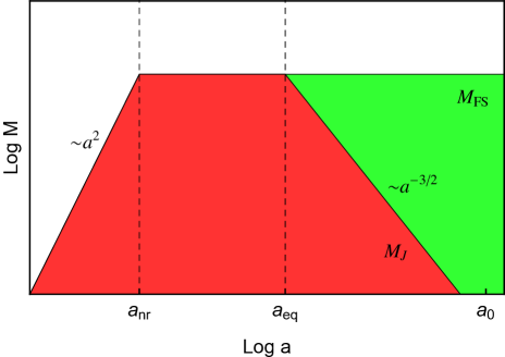
With the help of Eq. (4), it is now straight forward to qualitatively trace the evolution of the Jeans criterion through cosmic history: In the very early universe the dark matter component is still relativistic ($\sigma_{\rm v}\sim c$) and the Jeans mass is growing. As soon as the dark matter becomes non relativistic, its thermal velocity dispersion cools in the Hubble flow ($\sigma_{\rm v}\sim a^{-1}$) and the Jeans mass becomes approximately constant; during this still radiation-dominated era, $\bar{\rho}\sim a^{-4}$ while $\rho_{\rm m}\sim a^{-3}$. This is the case until about matter-radiation equality, where the evolution of the background density changes and the Jeans mass drops significantly.

As soon as a mass scale becomes Jeans stable, all perturbations below this mass scale are damped to zero. The free streaming scale can therefore alternatively be defined as the maximum value of the Jeans mass in cosmic history. This is usually the case around matter-radiation equality, where the Jeans scale happens to be of the order of the free streaming scale defined in Eq. (2).

The evolution of the Jeans mass and the corresponding free streaming mass is summarized in Fig. 1, where the red coloured area represents scales with strictly no growing solutions, while the green coloured region stands for scales with growing solutions but erased initial perturbations. While the Jeans and the free streaming mass are comparable until matter-radiation equality, they differ substantially in scale today.

2.1 Power spectrum

A detailed calculation of the effects of the free streaming on the power spectrum of initial perturbations can only be obtained by solving the coupled linearized Einstein-Boltzmann equations for all relevant species in the Universe. The result is usually given in terms of a transfer function, which is a mapping of the primordial perturbations from the end of inflation to the moment when the first perturbations become nonlinear.

In the case of a WDM universe several transfer functions have been proposed, taking into account different production mechanisms for the dark matter particle. In the following we use the formula presented in Viel et al. (2005):

$$T_{\rm WDM}(k)=\left[\frac{P_{\rm lin}^{\rm WDM}}{P_{\rm lin}^{\rm CDM}}\right]^{1/2}=\left[1+(\alpha k)^{2\mu}\right]^{-5/\mu},$$ (5)

with $\mu=1.12$ as well as

$$\alpha=0.049\left[\frac{m_{\rm WDM}}{{\rm keV}}\right]^{-1.11}\left[\frac{\Omega_{\rm WDM}}{0.25}\right]^{0.11}\left[\frac{h}{0.7}\right]^{1.22}\,h^{-1}{\rm Mpc},$$ (6)

which holds for a thermally produced dark matter candidate. A direct translation to the mass of a sterile neutrino is given by the fitting function

$$m_{\nu_{s}}=4.43{\rm keV}\left(\frac{m_{\rm WDM}}{1{\rm keV}}\right)^{4/3}\left(\frac{\Omega_{\rm WDM}}{0.1225}\right)^{-1/3}.$$ (7)

The WDM free streaming introduces a characteristic scale of suppression, and it is convenient to define it to be the ‘half-mode’ scale at which the WDM transfer function drops to $1/2$ (Schneider et al., 2012). The half-mode mass scale is given by

$$M_{\rm WDM}^{\rm hm}=\frac{4\pi}{3}\bar{\rho}\left[\pi\alpha\left(2^{\mu/5}-1\right)^{-\frac{1}{2\mu}}\right]^{3}.$$ (8)

and is about at the mass scale of a dwarf galaxy, depending on the exact WDM particle mass.

In the case of a CDM cosmology with a neutralino dark matter candidate, the free streaming cutoff scale is much smaller. The transfer function obtained by Green et al. (2004) has the form

$$T_{\rm N}(k)=\left[1-\frac{2}{3}\left(\frac{k}{k_{\rm A}}\right)^{2}\right]\exp\left[-\left(\frac{k}{k_{\rm A}}\right)^{2}-\left(\frac{k}{k_{\rm B}}\right)^{2}\right]$$ (9)

where

$$k_{\rm A} = 2.4\times 10^{6}\left(\frac{m_{\rm N}}{100\rm GeV}\right)^{1/2}$$ (10)

$$\times\frac{\left(T_{\rm kd}/30\rm MeV\right)^{1/2}}{1+\log(T_{\rm kd}/30\rm MeV)/19.2}[\,h\,{\rm Mpc}^{-1}]\ ,$$

$$k_{\rm B}=5.4\times 10^{7}\left(\frac{m_{\rm N}}{100\rm GeV}\right)^{1/2}\left(\frac{T_{\rm kd}}{30\rm MeV}\right)^{1/2}[\,h\,{\rm Mpc}^{-1}],$$ (11)

where $T_{\rm kd}$ is the kinetic decoupling temperature, which depends on the specific parameters of the supersymmetric model. Typical values for $T_{\rm kd}$ vary between 20 MeV and 35 MeV, but more extreme values are possible (see Green et al., 2005, for more details).

Owing to the fact that Eq. (9) is not algebraically solvable for $k$, an expression for the half-mode scale cannot be given. However, for a 100 GeV neutralino with a decoupling temperature of 30 MeV the half-mode mass is $M=2.9\times 10^{-6}h^{-1}M_{\odot}$, which roughly corresponds to the mass of the Earth.

Sim label	$L\,[\,h^{-1}{\rm Mpc}]$	$N_{\rm sim}$	RS	$m_{\rm WDM}\,[{\rm keV}]$	$M_{\rm hm}[h^{-1}M_{\odot}]$	$m_{p}\,[h^{-1}M_{\odot}]$	$l_{\rm soft}[\,h^{-1}{\rm kpc}]$
CDM_L256	256	$1024^{3}$	345897	$\infty$	0	$1.18\times 10^{9}$	5.00
CDM_L64	64	$1024^{3}$	345897	$\infty$	0	$1.83\times 10^{7}$	1.25
CDM_L16	16	$1024^{3}$	345897	$\infty$	0	$2.86\times 10^{5}$	0.31
WDM_m1.0_L256	256	$1024^{3}$	345897	1.0	$1.3\times 10^{10}$	$1.18\times 10^{9}$	5.00
WDM_m1.0_L64	64	$1024^{3}$	345897	1.0	$1.3\times 10^{10}$	$1.83\times 10^{7}$	1.25
WDM_m1.0_L16a	16	$1024^{3}$	345897	1.0	$1.3\times 10^{10}$	$2.86\times 10^{5}$	0.31
WDM_m1.0_L16b	16	$1024^{3}$	234786	1.0	$1.3\times 10^{10}$	$2.86\times 10^{5}$	0.31
WDM_m1.0_L16c	16	$1024^{3}$	123675	1.0	$1.3\times 10^{10}$	$2.86\times 10^{5}$	0.31
WDM_m0.5_L256	256	$1024^{3}$	345897	0.5	$1.3\times 10^{11}$	$1.18\times 10^{9}$	5.00
WDM_m0.5_L64	64	$1024^{3}$	345897	0.5	$1.3\times 10^{11}$	$1.83\times 10^{7}$	1.25
WDM_m0.25_L256	256	$1024^{3}$	345897	0.25	$1.3\times 10^{12}$	$1.18\times 10^{9}$	5.00
WDM_m0.25_L64a	64	$1024^{3}$	345897	0.25	$1.3\times 10^{12}$	$1.83\times 10^{7}$	1.25
WDM_m0.25_L64b	64	$1024^{3}$	234786	0.25	$1.3\times 10^{12}$	$1.83\times 10^{7}$	1.25
WDM_m0.25_L64c	64	$1024^{3}$	123675	0.25	$1.3\times 10^{12}$	$1.83\times 10^{7}$	1.25
WDM_m0.25_L64d	64	$1024^{3}$	012564	0.25	$1.3\times 10^{12}$	$1.83\times 10^{7}$	1.25

Table 1: Numerical simulations used in this paper. Columns from left to right: simulation name; simulation box-size ($L$); particle number ($N_{\rm sim}$); random seed number (RS); mass of WDM particle ($m_{\rm WDM}$); half-mode mass-scale ($M_{\rm hm}$); mass of simulation particles $(m_{\rm p})$; comoving softening length ($l_{\rm soft}$). The simulations with $L=256\,h^{-1}{\rm Mpc}$ have already been published in Schneider et al. (2012).

2.2 The role of late time velocities

Numerical simulations of cosmologies with a non negligible free streaming length are usually done by simply assuming a cutoff in the initial power spectra (as discussed above) without directly including thermal velocities in the numerical simulations. This approach has been applied for simulations in WDM (Bode et al., 2001; Lovell et al., 2011; Schneider et al., 2012) as well as simulations of tiny high redshift boxes in CDM (Diemand et al., 2005; Ishiyama et al., 2010; Anderhalden & Diemand, 2013). Neglecting the late time thermal velocity contribution is a good approximation as long as the Jeans mass is well below the mass resolution at the initial redshift of the simulation.

After matter-radiation equality at $z_{\rm eq}\sim 3200$, the overdensities grow significantly while the Jeans mass drops with a rate of $M_{\rm J}\sim a^{-3/2}$ (as discussed in §2 and in the corresponding Fig. 1). This means that already at $z\sim 600$ the Jeans mass is more than one order of magnitude and at $z\sim 100$ more than two orders of magnitude below the free streaming scale. For simulations with a typical starting redshift of $z\sim 100$, it is therefore impossible to see a direct effect of initial particle thermal velocities on the WDM mass function – the artificial clumping scale would be orders of magnitude larger than the thermal velocity Jeans scale at the initial epoch of the simulation. This also holds for halo density profiles, where the effects of thermal velocities (transformation of halo cusps into central cores) are only observable if the late time velocities are artificially boosted (Villaescusa-Navarro & Dalal, 2011; Maccio et al., 2012; Shao et al., 2013).

Benson et al. (2012) included the effect of late time thermal velocities into their mass function calculation and found a very prominent effect, which changes the shape of the mass function at scales around the cutoff. Their model is based on work of Barkana et al. (2001), who included the effect of velocities in an isolated simulation of spherical collapse. The starting redshift of the Barkana et al. simulation, however, is at matter-radiation equality, at a time where all relevant perturbations are still extremely small and deep in the linear regime. Their spherical collapse simulation can therefore be understood as a simplified method to solve the linear Boltzmann equation (where velocities have been included as well; see for example Viel et al., 2005) and, not surprisingly, leads to a cutoff at about the same scale as the cutoff in the WDM transfer function. Starting the spherical collapse much later at a redshift just before the relevant modes become nonlinear, would strongly reduce the influence of the thermal velocities and would push the effect on the mass function to much smaller scales, orders of magnitude below the relevant half-mode scale of Eq. (8).

3 Simulating the WDM universe

In this section we present our set of WDM simulations and give details about the initial conditions, the gravity code, and the characteristics of the individual runs. In a second part we then discuss the issue of artificial clumping in detail and develop a way to deal with it for the purpose of the halo mass function.

3.1 Characteristics of the simulations

For all our simulations we used a WMAP7 cosmology with the parameters $\Omega_{\rm m}=0.2726$, $\Omega_{\Lambda}=0.7274$, $\Omega_{\rm b}=0.046$, $h=0.704$, $n_{s}=0.963$, and $\sigma_{8}=0.809$ (Komatsu et al., 2011). The CDM transfer function was generated with the CAMB code of Lewis et al. (2000). For the initial conditions we used the 2LPT code (Scoccimarro, 1998; Crocce et al., 2006) with an initial redshift of $z_{\rm IC}=49$ for runs with box size $L=256\,\,h^{-1}{\rm Mpc}$ and $z_{\rm IC}=99$ for runs with box sizes $L=64\,\,h^{-1}{\rm Mpc}$ and $L=16\,\,h^{-1}{\rm Mpc}$. All simulations have been performed with PKDGRAV, a treecode with high order multipole expansion and adaptive timestepping (Stadel, 2001).

A summary of all simulations including some important physical and numerical quantities is listed in Table 1. All simulations have $1024^{3}$ particles. The simulations with boxsize $L=256\,\,h^{-1}{\rm Mpc}$ have already been published in Schneider et al. (2012), the others have been performed during the last year on the SuperMUC cluster in Munich and the CSCS cluster in Lugano. For the instructive purposes of resolving halo formation well below the cutoff scale, we focus on cosmologies somewhat warmer than the canonical 2 keV WDM candidate.

The halo finding was done using a friends-of-friends (FoF) algorithm (Davis et al., 1985) provided by the $N$-Body Shop, with the usual linking length of $b=0.2$ and with no unbinding of haloes.

For the smallest boxes of $L=16\,\,h^{-1}{\rm Mpc}$ we performed a finite volume correction to compensate for the missing large-power modes. This was done in the simplest way by truncating the integrals present in Eqs (15) and (16) at scales larger than the box length, taking the ratio of the truncated to non-truncated mass function and multiplying this ratio to the simulation measurements (see for example Watson et al., 2012). Whilst this simple correction neglects the effects of the discrete Fourier mode distribution and the run to run sample variance of each realization, the resulting corrected mass function is similar to that obtained using the correction technique of Reed et al. (2007). The result is an increase in the abundance of haloes at large mass scales, and, somewhat counter intuitively, a decrease in the abundance of haloes for smaller mass scales. For the larger boxes $L=\{64,256\}\,\,h^{-1}{\rm Mpc}$, no finite volume correction has been implemented, since it has an negligible influence on the halo abundance.

3.2 Artificial haloes and resolution

Numerical simulations of cosmologies with truncated initial power spectrum produce artificial clumping at scales beyond the cutoff. In the simulation outputs these artefacts are most visible in cosmic filaments, where they form equally spaced clumps that are strongly resolution dependent (Wang & White, 2007; Schneider et al., 2012). They seem however to be present in all environments from underdense voids to high density clusters and therefore cannot simply be cut out of the simulation analysis.

In the halo mass function the artificial clumps appear as a steep power-law, which leads to a prominent upturn below a characteristic mass scale. In Fig. 2 we plot the mass function of all simulated boxes together with the usual Sheth-Torman prediction (dashed lines). The different colours correspond to different cosmologies (black: CDM, red: $m_{\rm WDM}=1.0\,{\rm keV}$, green: $m_{\rm WDM}=0.5\,{\rm keV}$, blue: $m_{\rm WDM}=0.25\,{\rm keV}$), the symbols denote the box size of the simulations (circles: $L=256\,h^{-1}{\rm Mpc}$, triangles: $L=64\,\,h^{-1}{\rm Mpc}$; squares: $L=16\,\,h^{-1}{\rm Mpc}$).

Figure 2: Redshift zero mass functions measured in our simulations. Black is the CDM cosmology, blue, green and red are WDM cosmologies with particle masses of $m_{\rm WDM}\in\{0.25,0.5,1.0\}\,{\rm keV}$. Circles correspond to simulations with $L=256\,\,h^{-1}{\rm Mpc}$, triangles to simulations with $L=64\,\,h^{-1}{\rm Mpc}$ and squares to simulations with $L=16\,\,h^{-1}{\rm Mpc}$ (each with $1024^{3}$ particles). The low mass upturn in the WDM runs is due to spurious structures. The dashed lines represent the usual Sheth-Torman mass function.

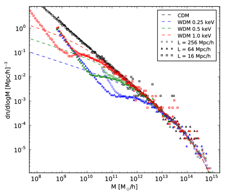
The figure clearly shows the dependence of the artifical upturn of the mass function on the resolution of the simulation. Furthermore, we note that the mass function of the artificial clumps display a power-law behaviour. Interestingly, the power-law index of the artificial mass function does not appear to depend strongly on the mass of the WDM particle. Instead, it becomes more negative with decreasing resolution.

The presence of the artificial clumping is a very serious problem for numerical simulations, since increasing the resolution becomes tremendously expensive. Wang & White (2007) noticed that the effective converging resolution only goes as $N^{1/3}$ with increasing particle number $N$. However, as Fig. 2 shows things are even worse than that, because the slope of artificial upturn becomes shallower as the simulation resolution increases, which makes it more difficult to distinguish between the artificial and real part of the mass function. Also, it is not possible to simply shrink the box size of the simulation to increase the mass resolution. Owing to the flatness of the WDM mass function, small boxes simply do not have enough haloes to get a statistically meaningful result. The combination of all these effects makes it incredibly challenging to probe mass scales significantly below the half-mode mass scale. It is therefore crucial to attempt to obtain an improved theoretical understanding of how the mass function behaves at these scales.

Additionally to the resolution problems mentioned above, the exact scale of the artificial upturn is not always easy to determine. It is possible that there are still physical haloes in the artificially driven power-law part of the mass function. On the other hand the power-law of artificial clumps could extend to higher masses than what is apparent and change the shape of the mass function at scales well above the visible upturn.

3.3 Artificial haloes and environment

In order to examine the distribution of artificial haloes, we measure the mass function in different environments. If the visual impression that the artefacts lie predominantly in filaments is correct, then it should be possible to extract the halo mass function down to smaller mass scales by exclusively looking in very underdense void-like environments.

We measure what we will refer to as an “approximate conditional mass function” by imposing a halo isolation criteria. In practice, we choose a specific nearest neighbour isolation criterion and only retaining ‘isolated’ haloes whose nearest neighbour is further away than the distance $d$, defined in units of the box size $L$. This gives an approximate measure of the underdense conditional mass function. ‘Non-isolated’ haloes on the other hand – the ones with at least one neighbour closer than $d$ – can be used to approximate an overdense conditional mass function.

In Fig. 3 we plot the approximate conditional mass function of various overdense and underdense environments with varying distance $d$. The mass function measurements are normalized in a way that an integration over all mass bins leads to the same effective halo number – i.e. the measured mass function in a certain environment $dn_{\rm env}/d\log M$ is multiplied with the ratio $N_{\rm env}/N_{\rm tot}$, where $N_{\rm env}$ and $N_{\rm tot}$ are the total number of haloes in the specific environment and in the whole box, respectively. As expected from visual appearances, the underdense regions are less contaminated with spurious haloes than the unconditional mass function, as indicated by the mass scale of the artificial upturn. Overdense regions on the other hand, have more artefacts and the artificial upturn therefore happens at larger masses. The power-law slope of associated with the artificial haloes, seems to be independent of environment (c.f. Fig. 2, and even the WDM model).

Figure 3: Approximate conditional mass function of underdense and overdense environments for the $m_{\rm WDM}=0.25\,{\rm keV}$ model. Haloes in underdense (overdense) regions have no (at least one) neighbour within the distance $d$, defined in units of the box size $L$. The artificial upturn is shifted to smaller (larger) masses in underdense (overdense) regions. The power-law of the artificial haloes seems to be independent of the environment. The halo environment is defined via the distance to the nearest neigbour $d$.

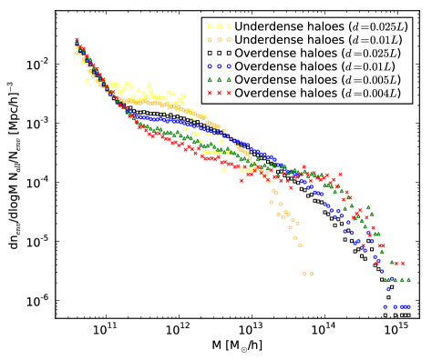
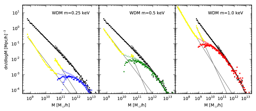
The fact that the power-law of artefacts is ‘exposed’ up to larger masses in overdense regions means that it must extend far beyond the visible upturn even in the unconditional mass function. By extension, it also implies that some of the haloes in the artificial upturn must be real. In order to get a meaningful approximation of the physical mass function, the artificial power-law should therefore be subtracted from the measurements. We do this by individually fitting a separate power-law function to the artificial part of every simulation and then subtract this power-law function from the measurements. The artificial part is determined via a visible inspection and consists of the data points that are clearly above the upturn, where the shape of the mass function is a pure power law. This approach of subtracting artefacts allows us to get a meaningful mass function down to the mass scale where the artificial upturn is a pure power-law. However, it is important to note that this involves an extrapolation of the spurious halo mass function to large mass scales.

In Fig. 4 the corrected mass function with power-law subtraction is plotted in solid bold symbols while the faint symbols corresponds to the original non-corrected mass function. The left panel shows the measured mass function of the WDM run with $m_{\rm WDM}=0.25\,{\rm keV}$ (blue), the middle panel the WDM run with $m_{\rm WDM}=0.5\,{\rm keV}$ (green) and the right panel the WDM run with $m_{\rm WDM}=1.0\,{\rm keV}$ (red). The power laws, which are subtracted from the original mass function, are plotted as grey lines and the fitting of these lines is done over the yellow symbols.

Figure 4: Correction of WDM mass functions for the effects of spurious structure formation in the simulations. Left panel: WDM with $m_{\rm WDM}=0.25\,{\rm keV}$, middle panel: WDM with $m_{\rm WDM}=0.5\,{\rm keV}$, right panel: WDM with $m_{\rm WDM}=1.0\,{\rm keV}$. The CDM measurements have been added to every panel for comparison. The faint symbols correspond to the original mass function, the bold symbols correspond to the corrected mass function. The grey lines are the power-laws which are subtracted. The fitting is done over the yellow symbols. The WDM mass function decreases towards low masses only when this correction is applied.

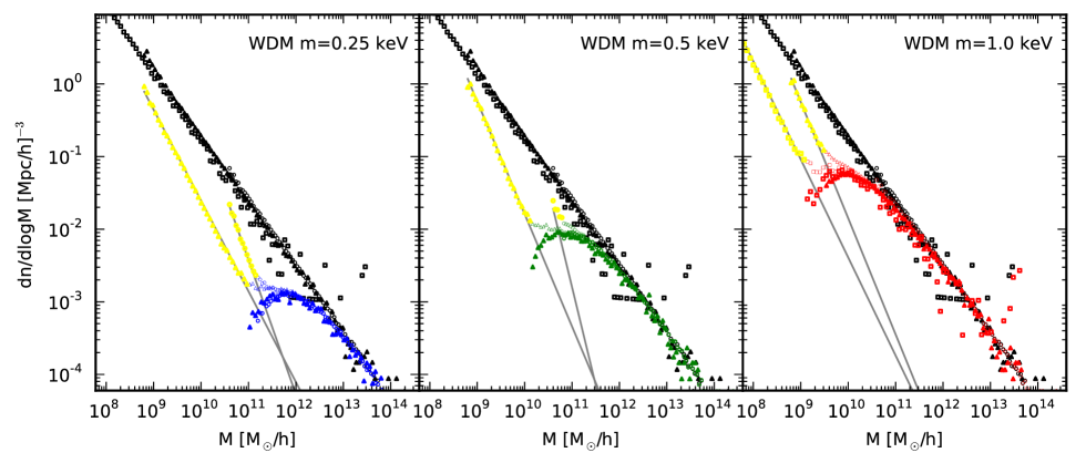
In the following we will only consider the corrected measurement of the mass function and use it to calibrate our analytical approaches.

4 Mass Function in a WDM Universe

The EPS framework (Press & Schechter, 1974; Bond et al., 1991; Lacey & Cole, 1993; Musso & Sheth, 2012) captures many important features of the end states of structure formation in the CDM model. In particular, the halo mass function can be defined as

$$\frac{dn}{d\log M}=-\frac{1}{2}\frac{\bar{\rho}}{M}f(\nu)\frac{d\log\sigma^{2}}{d\log M}\ .$$ (12)

where $f(\nu)$ is the first crossing distribution, $\sigma^{2}(M)$ the variance at the mass scale $M$, and $\bar{\rho}$ is the average density of the universe. On assuming uncorrelated random-walks and a collapse barrier set by the spherical collapse model, the excursion set model predicts (Press & Schechter, 1974; Bond et al., 1991):

$$f(\nu)=\sqrt{\frac{2\nu}{\pi}}e^{-\nu/2},\hskip 14.22636pt\nu\equiv\frac{\delta_{c}^{2}(t)}{\sigma^{2}(M)}\ ,$$ (13)

where $\delta_{c}(t)=1.686/D(t)$ is the linearly extrapolated density for collapse in the spherical model and $D(t)$ is the growth factor normalized to be unity at $z=0$. An ellipsoidal collapse barrier gives

$$f(\nu)=A\sqrt{\frac{2q\nu}{\pi}}\left[1+(q\nu)^{-p}\right]e^{-q\nu/2},$$ (14)

where ${p=0.3}$ and ${A=0.3222}$ (Sheth & Tormen, 1999). The third parameter $q$ is predicted to be one in the ellipsoidal approach, but Sheth & Tormen realized that the cluster abundance in simulations is better matched with the empirical value $q=0.707$.

In this framework all of the sensitivity of the mass function to cosmology is encoded in the variance of the density perturbations on a given scale $R$. The variance can be expressed as

$$\sigma^{2}(R)=\int\frac{{\rm d}^{3}{\bf k}}{(2\pi)^{3}}P_{\rm Lin}(k)W^{2}(kR)\ ,$$ (15)

where $P_{\rm Lin}$ is the linear theory matter power spectrum at $z=0$ and $W$ is the Fourier transform of the filter function. Note that in the EPS framework the predictions are unchanged if we consider, rather than the density field growing with time and points collapsing when they cross a given density threshold, the collapse barrier evolves with time and the field remains static. We adopt this latter convention. Consequently, it means that the cosmological information encoded in the growth of the power spectrum is transferred to $\delta_{\rm c}(t)$. Note also that the value of $\delta_{\rm c}$ itself has a weak cosmology dependence (Lahav et al., 1991; Eke et al., 1996), however in what follows this shall be neglected.

In the case of perfectly cold dark matter, $\sigma^{2}(R)$ rises monotonically towards smaller $R$ and becomes infinite as $R\rightarrow 0$. On the other hand if free streaming takes place, the variance becomes constant for small but finite $R$, since the cutoff in the power spectrum truncates Eq. (15).

In order to evaluate Eq. (12) we also require the logarithmic derivative of the variance with respect to the mass scale, given by

$$\frac{d\log\sigma^{2}}{d\log M}=\frac{2}{3\sigma^{2}}\int\frac{{\rm d}^{3}{\bf k}}{(2\pi)^{3}}P_{\rm Lin}(k)W(kR)\frac{dW(kR)}{d\log(kR)}.$$ (16)

For scales well above the half-mode scale, the behaviour of this expression is almost independent of the exact choice of the window function. However, this changes quite dramatically as one approaches the half-mode scale, whereupon the choice of the window function dictates the asymptotical behaviour of Eq. (16), and thereby determines the shape of the mass function at low masses.

4.1 Choosing the right window function

In the presence of particle free streaming the mass function strongly depends on the choice of the window function. Some common filter functions are the following:

• Tophat window: This filter has the form of a sphere with radius $R_{\rm TH}$ and sharp boundaries in real space and therefore has an obvious mass assignment $M_{\rm TH}=4\pi\bar{\rho}R_{\rm TH}^{3}/3$. In Fourier space this window has the form:

  $$W_{\rm TH}(y)=\frac{3}{y}\left[\sin y-y\cos y\right],\hskip 28.45274pty=kR_{\rm TH}.$$ (17)

  The downside of the spherical tophat filter is that in Fourier space the random walk is correlated and the first crossing distribution cannot be recovered analytically (Bond et al., 1991; Maggiore & Riotto, 2010).

• Gaussian window: This filter has no sharp boundaries but the characteristic form of a Gaussian (with variance $R_{\rm GA}^{2}$) in real space. In Fourier space this property is maintained, leading to

  $$W_{\rm GA}(y)={\rm{e}}^{-y^{2}/2},\hskip 28.45274pty=kR_{\rm GA}.$$ (18)

  A Gaussian window gives somewhat smoother results than a simple tophat window, but it has the drawback of not having a well defined mass. The most common practice to assign a mass is to normalize the filter to one in real space and to integrate over the filter volume. Multiplying the volume with the average density then leads to a filter mass of $M_{\rm GA}=(2\pi)^{3/2}\pi\bar{\rho}R_{\rm GA}^{3}$. The normalization is however arbitrary and this introduces an ambiguity into the mass assignment (Maggiore & Riotto, 2010).

• Sharp-$k$ window: This filter is defined as a tophat sphere in Fourier space:

  $$W_{\rm SK}(y)=\Theta(1-y),\hskip 28.45274pty=kR_{\rm SK},$$ (19)

  and has the very appealing property that the steps of the random walk are uncorrelated for a Gaussian field. The drawback is its wiggly shape in real space, leading to contributions on all scales and making it difficult to find a reasonable mass assignment. The same procedure as for the Gaussian filter – i.e. normalizing the filter and integrating over the enclosed volume – leads to a divergent integral (Maggiore & Riotto, 2010). Apart from the $M_{\rm SK}\propto R_{\rm SK}^{3}$ proportionality, the mass assignment is therefore basically unconstrained and needs to be chosen by comparing to simulations (a more detailed discussion on the sharp-$k$ mass assignment is given in §4.3).

We now look at the effect of the different windows on the behaviour of the mass function in a universe including free streaming. The filter specific mass function can be written as

$$\frac{dn_{\alpha}}{d\log M_{\alpha}}=\frac{1}{2}\frac{\bar{\rho}}{M_{\alpha}}f_{\alpha}(\nu_{\alpha})\left|\frac{d\log\sigma^{2}_{\alpha}}{d\log M_{\alpha}}\right|,\hskip 14.22636pt\nu_{\alpha}=\frac{\delta^{2}_{\rm c}}{\sigma^{2}_{\alpha}},$$ (20)

where the index $\alpha$ refers to a particular window function, e.g. $\alpha\in\{\rm TH,\,GA,\,SK\}$, and so for instance $f_{\rm TH}(\nu_{\rm TH})$ is the first crossing distribution computed using the spherical top-hat window function.

In the small scale limit below the half-mode scale the variance given in Eq. (15) becomes constant and the asymptotical behaviour of the mass function of Eq. (20) is therefore given by

$$\lim\limits_{R_{\alpha}\rightarrow 0}{\frac{dn_{\alpha}}{d\log M_{\alpha}}}\propto\frac{1}{R_{\alpha}^{3}}\lim\limits_{R_{\alpha}\rightarrow 0}{\frac{d\log\sigma_{\alpha}^{2}}{d\log M_{\alpha}}}.$$ (21)

It is now straight forward to calculate the asymptotical behaviour of the mass function for different filter choices. In the case of a tophat window and equivalently of a Gaussian window we obtain

$$\lim\limits_{R_{\alpha}\rightarrow 0}{\frac{dn_{\alpha}}{d\log M_{\alpha}}}\propto\lim\limits_{R_{\alpha}\rightarrow 0}R_{\alpha}^{-1}=\infty,\hskip 14.22636pt\alpha=\rm{TH},\rm{GA}$$ (22)

which means that the mass functions of these filters diverge for small scales. This result is in contradiction to our understanding of structure formation around and below the half-mode mass scale. However, In the case of a sharp-$k$ window the asymptotical behaviour of the mass function is given by

$$\lim\limits_{R_{\rm SK}\rightarrow 0}{\frac{dn_{\rm SK}}{d\log M_{\rm SK}}} \propto \lim\limits_{R_{\rm SK}\rightarrow 0}R_{\rm SK}^{-6}P_{\rm Lin}\left(\frac{1}{R_{\rm SK}}\right)$$ (23)

$$\simeq \lim\limits_{R_{\rm SK}\rightarrow 0}R^{18-n}=0\ .$$

In obtaining the last line we have used

$$P_{\rm Lin}(1/R_{\rm SK})\propto R_{\rm SK}^{-n}T^{2}_{\rm CDM}(1/R_{\rm SK})T_{\rm WDM}^{2}(1/R_{\rm SK})\ .$$ (24)

The asymptotical behaviour of the sharp-$k$ mass function has the correct physical characteristics – it becomes strongly suppressed around the scales where free streaming is dominant. Owing to this and the fact that the first crossing distribution was derived for the sharp-$k$ window, we will adopt this window function throughout the rest of this paper. However, we are still left with the task of how we assign mass to this filter function. We shall discuss this issue in §4.3.

4.2 Mass function with sharp-$k$ window

It is now straight forward to derive an expression for the halo mass function based on the sharp-$k$ window function. Since the logarithmic derivative of the window is

$$\frac{dW_{\rm SK}}{d\log y}=-y\delta^{D}(1-y),\hskip 28.45274pty=kR_{\rm SK},$$ (25)

where $\delta^{D}$ is the Dirac delta function, we can evaluate the integral in Eq. (16), obtaining

$$\frac{d\log\sigma_{\rm SK}^{2}}{d\log R_{\rm SK}}=-\frac{1}{2\pi^{2}\sigma_{\rm SK}^{2}(R_{\rm SK})}\frac{P_{\rm Lin}(1/R_{\rm SK})}{R_{\rm SK}^{3}}.$$ (26)

Here we have used the fact that $\Theta(0)=1/2$. We can now implement Eq. (26) into the relation

$$\frac{dn_{\rm SK}}{d\log M_{\rm SK}}=-\frac{1}{2}\frac{\bar{\rho}}{M_{\rm SK}}f_{\rm SK}(\nu_{\rm SK})\frac{d\log\sigma_{\rm SK}^{2}}{d\log R_{\rm SK}}\frac{d\log R_{\rm SK}}{d\log M_{\rm SK}},$$ (27)

to obtain the mass function based on the sharp-$k$ window function. Note that provided $M_{\rm SK}\propto R_{\rm SK}^{3}$ the term $d\log M_{\rm SK}/d\log R_{\rm SK}=3$.

With an appropriate mass assignment, Eq. (27) gives a very good match to the measurements of both the CDM and the WDM simulations. Especially the flattening and the turnover in the WDM mass function can be described accurately. A direct comparison to the simulations is done in §4.4.

4.3 Mass assignment

In the previous sections we mentioned that the sharp-$k$ window function has no well defined mass assigned to its filter scale. This intrinsic ambiguity can be exploited by choosing a mass assignment that yields a good agreement with simulations. Owing to the geometrical scaling of halo mass with radius (at fixed virial halo density), it is however a reasonable assumption to maintain the $M\propto R_{\rm SK}^{3}$ proportionality and we can therefore write

$$M_{\rm SK}=\frac{4\pi}{3}\bar{\rho}\left[cR_{\rm SK}\right]^{3}=\frac{M_{\rm TH}}{c^{3}},$$ (28)

where $c=R_{\rm TH}/R_{\rm SK}$ is a free constant. Lacey & Cole (1993) proposed the value $c=(9\pi/2)^{1/3}\simeq 2.42$, which can be obtained by normalizing the filter to one in real space and integrating over the volume. One part of this integral is however diverging and Lacey & Cole set it to zero without any physical motivation (see Maggiore & Riotto, 2010, for a more detailed discussion). In this paper, we choose $c=2.7$, also without physical justification, in order to get an optimal match with our simulations. This value is not only larger than the one from Lacey & Cole (1993) but also slightly larger than the value $c=2.5$ used by Benson et al. (2012). The difference between our choice and the one of Benson et al. (2012) comes from the fact that we compare to the corrected mass function measurements (as explained in §3.3) while they compared to the direct measurement of the mass function and ignore all spurious haloes above the visible upturn.

Figure 5: Mass function with tophat filter (dashed) as well as sharp-$k$ filter with spherical mass assignment (dotted) and ellipsoidal correction (solid). For the spherical mass assignment we used $c=2.7$ and $q=1.0$, for the ellipsoidal correction we used $c_{\rm e}=2.0$ and $q=0.75$. A tophat window function produces a qualitatively incorrect mass function below the free streaming scale.

Furthermore, in order to obtain a good match with simulations we also set $q=1$ in Eq. (14). This means that with a sharp-$k$ filter we can use the first crossing distribution, which naturally arises from the EPS approach with ellipsoidal collapse and we do not need any further empirical shift of the crossing barrier. Thus, somewhat suprisingly, we find that neither the rescaling of the first crossing distribution of Sheth & Tormen (1999) nor the rescaling of the critical overdensity done by Benson et al. (2012) is necessary. From a theoretical perspective this means that our sharp-$k$ model is competitive with the spherical tophat model, since the additional free parameter from the mass assignment is counterbalanced by the use of a more natural first crossing distribution.

4.4 Comparison with simulations

The halo mass function predictions from Eq. (27) together with the mass assignment of Eq. (28) can now be compared to the simulated CDM and WDM scenarios. We do this for the entire mass range spanned by our simulations $M\in\left[10^{9},10^{15}\right]h^{-1}M_{\odot}$ and for redshifts $z=0$ and $z=4.4$. The redshift $z=4.4$ corresponds to the earliest output for which we have sufficiently good halo number statistics.

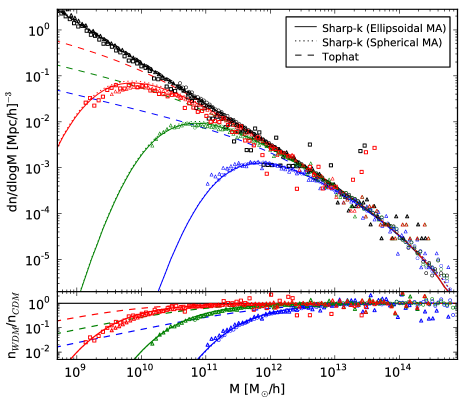
Fig. 5 shows the mass function at $z=0$, where the different dark matter models are distinguished by colour (black: CDM, blue: $m_{\rm WDM}=0.25\,{\rm keV}$, green: $m_{\rm WDM}=0.5\,{\rm keV}$, red: $m_{\rm WDM}=1.0\,{\rm keV}$). The symbols represent the simulation measurements, with the shape depending on the box size of the simulation (circle: $L=256\,\,h^{-1}{\rm Mpc}$, triangles: $L=64\,\,h^{-1}{\rm Mpc}$, squares: $L=16\,\,h^{-1}{\rm Mpc}$). The spherical tophat and sharp-$k$ mass functions are denoted by the dashed and dotted lines, respectively. The model represented by the solid line will be discussed in §4.5.

Figure 6: Mass functions at redshift 1.1 (left panel), 2.4 (middle panel) and 4.4 (right panel). Again, the tophat mass function is plotted as dashed line and the sharp-$k$ mass function as dotted line while the solid line represents the mass function with ellipticity correction, which enables a much better match to the simulations at high redshifts. All the labels are the same as in Fig. 5.

For the CDM cosmology, both the spherical tophat and the sharp-$k$ mass functions give very similar predictions. There is a small difference for very high masses, where the sharp-$k$ mass function predicts slightly more haloes. Numerical studies of the high mass end of the mass function give a halo abundance that lies in between the tophat and the sharp-$k$ model plotted here (Reed et al., 2007; Bhattacharya et al., 2011; Watson et al., 2012). However, and most importantly, the figure also shows that the predictions for the sharp-$k$ mass function are in good agreement with the WDM data. On the other hand, the standard spherical tophat approach significantly overpredicts the halo abundances at low masses and has the wrong asymptotical behaviour (see discussion in §4.1).

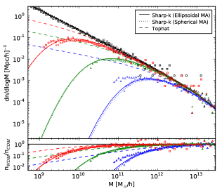
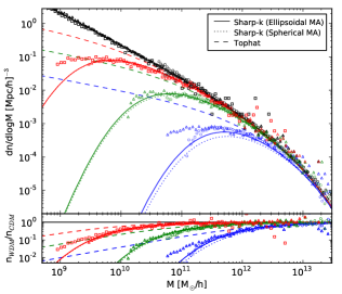
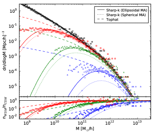
In Fig. 6 we plot the evolution of the mass function with redshift. The left, middle and right panels denote the results at $z=1.1$, 2.4 and 4.4, respectively. The line and symbol types are as in Fig. 5. Unfortunately, as one considers higher redshifts the sharp-$k$ model predictions begin to systematically underestimate the measured abundances. This seems to happen as soon as the WDM half-mode mass scale enters the exponential tail of the mass function. At $z=2.4$ and $z=4.4$ the exponential drop-off starts at a mass scale of $10^{11}$ M_⊙/h and $10^{10}$ M_⊙/h, respectively. Models with M${}^{\rm hm}_{\rm WDM}$ below this drop-off scale reproduce the simulation data well, while the ones above significantly under-predict the amount of haloes. The effect is most noticeable in the extreme WDM model (blue: $m_{\rm WDM}=0.25\,{\rm keV}$) at $z=4.4$ (right hand panel), where the discrepancy between model and data is nearly one order of magnitude. For a WDM model with more realistic particle mass, $m_{\rm WDM}>1{\rm keV}$, the effect is small and only becomes significant at very high redshifts. For example our most conservative WDM model (red: $m_{\rm WDM}=1\,{\rm keV}$) seems to be reasonably well matched at $z=1.1$ and $z=2.4$, and by $z=4.4$ there is only a slight under-prediction (visible in the absolute plot but not in the ratio plot).

We conclude that the sharp-$k$ mass function, as given by Eq. (27) with mass assignment from Eq. (28), seems to provide a reasonable match to simulation measurements at lower redshifts. However, the halo abundance of realistic WDM models with $m_{\rm WDM}>1\,{\rm keV}$ is likely to be systematically underestimated somewhere above $z>5$, when the half-mode mass scale M${}^{\rm hm}_{\rm WDM}$ enters the exponential tail of the mass function.

In the next section we propose that an ellipticity correction of the sharp-$k$ filter is required. On taking this into account we are able to obtain predictions that better describe the data for the entire range of halo masses, redshifts and WDM dark matter particle masses that we consider in this work.

4.5 Ellipticity correction

One possible explanation for the break down of the sharp-$k$ mass function predictions for WDM model at high redshifts, could be that the initial patches of a Gaussian random field are ellipsoidal, whereas the filter function is spherical and so at best characterises the effective radius of the patch. The ellipticity of the patches change both with size and redshift, being more spherical (ellipsoidal) for large (small) mass scales and at higher (lower) redshift (Bardeen et al., 1986). In CDM, the effect of the ellipticity can be folded into the mass assignment. In WDM however, ellipticity becomes important as soon as the half-mode mass scale (or cutoff scale in Fourier space) is approached. At this scale only spherical perturbations survive, while ellipsoidal perturbations do not form because their shortest axis lies below the half-mode mass scale, where no power is left.

Correcting for the ellipticity of initial patches only affects the mass assignment and is independent of the first crossing distribution. The point is to take into account the discrepancy between a spherical filter and ellipsoidal patches, which is independent of the effect of ellipsoidal collapse, leading to the first crossing distribution of Sheth & Tormen (1999).

The distribution of patch shapes for a Gaussian random field was established by Bardeen et al. (1986), who found that the expected set of axis ratios could be described by:

$$\frac{a_{3}}{a_{1}}(R_{\alpha}) = \sqrt{\frac{1-3e_{\rm m}(R_{\alpha})+p_{\rm m}(R_{\alpha})}{1+3e_{\rm m}(R_{\alpha})+p_{\rm m}(R_{\alpha})}}\ ,$$ (29)

$$\frac{a_{3}}{a_{2}}(R_{\alpha}) = \sqrt{\frac{1-2p_{\rm m}(R_{\alpha})}{1+3e_{\rm m}(R_{\alpha})+p_{\rm m}(R_{\alpha})}}\ ,$$ (30)

where the ellipsoid axis ratios are defined such that $(a_{3}\leq a_{2}\leq a_{1})$ and where $e_{\rm m}$ and $p_{\rm m}$ are the ellipticity and prolateness parameters of an average ellipsoidal density perturbation, both of which depend on the filter scale $R_{\alpha}$. In Appendix A we summarize some results from that work, which are salient for our application. In particular, the definition of ellipticity and prolateness as well as their dependence on the filter scale $R_{\alpha}$ and redshift $z$ are presented.

Figure 7: Axes ratios $a_{3}/a_{1}$ (solid) and $a_{3}/a_{2}$ (dashed) at redshift 0 (left panel) and redshift 4.4 (right panel) of the initial linear perturbations of the matter density field. The colours represent the different dark matter models (black: CDM; blue: $m_{\rm WDM}=0.25\,{\rm keV}$; green: $m_{\rm WDM}=0.5\,{\rm keV}$; red: $m_{\rm WDM}=1.0\,{\rm keV}$)

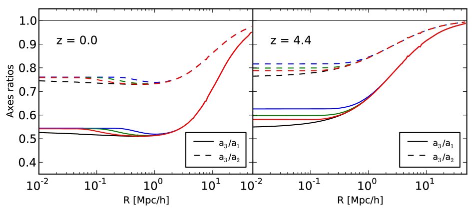
In Fig. 7 we show the evolution of the expected axis ratios for a sharp-$k$ filter as described by Eqns (29) and (30). The left and right panels show the results at $z=0$ and $z=4.4$, respectively, while the solid and dashed lines correspond to the ratios $a_{3}/a_{1}$ and $a_{3}/a_{2}$. The colours represent the different dark matter scenarios (black: CDM; blue: $m_{\rm WDM}=0.25\,{\rm keV}$; green: $m_{\rm WDM}=0.5\,{\rm keV}$; red: $m_{\rm WDM}=1.0\,{\rm keV}$). The patches are clearly more spherical at large scales and at high redshifts. Also the power spectrum of the WDM model leads to more spherical patches close to the cutoff scale.

For the case of the sharp-$k$ filter, the connection between the average radius $R_{\rm SK}$ and the shortest ellipsoidal axis $a_{3}$ can be obtained by comparing the volume of the filter to the exact volume of the ellipsoidal patch:

$$R_{\rm SK}^{3}=a_{1}a_{2}a_{3}=\left(\frac{a_{1}}{a_{3}}\frac{a_{2}}{a_{3}}\right)a_{3}^{3}=\left(\xi a_{3}\right)^{3},$$ (31)

where the ratios $a_{1}/a_{3}$ and $a_{2}/a_{3}$ and therefore $\xi$ depend on $R_{\rm SK}$. On combining Eqns (29), (30) and (31) we get

$$a_{3}(R_{\rm SK}) =\frac{R_{\rm SK}}{\xi(R_{\rm SK})},$$ (32)

$$\xi(R_{\rm SK}) =\left[\frac{(1+3p_{\rm m}+p_{\rm m})^{2}}{(1-3e_{\rm m}+p_{\rm m})(1-2p_{\rm m})}\right]^{1/6}.$$ (33)

The function $a_{3}(R_{\rm SK})$ is bijective and can be easily inverted to obtain $R_{\rm SK}(a_{3})$.

Now that we have a relation between the average size of the patch measured by a spherical filter and the effective smallest ellipsoidal axis, we can rewrite the mass assignment:

$$M_{\rm e}=\frac{4\pi}{3}\bar{\rho}\left[c_{\rm e}R_{\rm SK}(a_{3})\right]^{3},$$ (34)

where $a_{3}$ is now used as the reference scale that connects the linear power spectrum to the final halo abundance. We now conjecture that as soon as $a_{3}$ is below the half-mode mass scale, the corresponding ellipsoid is likely to be erased by the free streaming, while a spherical filter measuring an average radius $R_{\rm SK}$, which is still above the half-mode mass scale, will count the ellipsoid as being existent.

With the replacement of the relevant filter scale from $R_{\rm SK}$ to $a_{3}$, the halo mass function can be constructed after the following recipe:

1. Compute the first crossing distribution $f_{\rm SK}(\nu_{\rm SK})$ as before, using the average patch radius to obtain $\nu_{\rm SK}=\delta_{c}^{2}/\sigma_{\rm SK}^{2}(M_{\rm SK})$. No adaption to the ellipticity needs to be made here, since shear ellipticity is already encapsulated in the EPS approach with evolving barrier.

2. Calculate the average ellipticity $e_{\rm m}$ and prolateness $p_{\rm m}$ with respect to $R_{\rm SK}$ as described in Appendix A. Determine $\xi(R_{\rm SK})$ and invert Eq. (32) to obtain $R_{\rm SK}(a_{3})$.

3. Determine $M_{\rm e}$ as well as $d\log\sigma_{\rm SK}^{2}/d\log a_{3}$ and $d\log M_{\rm e}/d\log a_{3}$.

4. Construct the mass function as follows:

   $$\frac{dn_{\rm SK}}{d\log M_{\rm e}} = -\frac{1}{2}\frac{\bar{\rho}}{M_{\rm e}}f(\nu)\frac{d\log\sigma_{\rm SK}^{2}}{d\log a_{3}}\frac{d\log a_{3}}{d\log M_{\rm e}},$$ (35)

   $$\frac{d\log\sigma_{\rm SK}^{2}}{d\log a_{3}} = -\frac{1}{2\pi^{2}\sigma_{\rm SK}^{2}(a_{3})}\frac{P_{\rm Lin}(1/a_{3})}{a_{3}^{3}},$$ (36)

   $$\frac{d\log M_{\rm e}}{d\log a_{3}} = \frac{3}{\xi(R_{\rm SK})}\frac{dR_{\rm SK}}{da_{3}}.$$ (37)

   Note that the last term $d\log M/d\log a_{3}$ is not exactly 3 anymore because we have dropped the $M\propto a_{3}^{3}$ proportionality in Eq. (34).

In order to obtain a good match with the simulations, we take $c_{\rm e}=2.0$ for the mass assignment as well as $q=0.75$ for the first crossing distribution presented in Eq. (14). This means on comparison with the usual spherical tophat Sheth-Tormen approach, our model, with ellipticity correction, has one additional free parameter. This comes from the undetermined relation between filter scale and mass inherent to the sharp-$k$ filter (see the discussion in §4.3).

The predictions for our sharp-$k$ mass function with an ellipticity correction are plotted as the solid lines in Fig. 5 and Fig. 6. At redshift zero the differences between the results from the sharp-$k$ models with spherical and ellipsoidal mass assignment are very small. At higher redshifts, however, the corrected ellipsoidal mass assignment model matches well the estimates from the simulations. It shows a small under-prediction relative to the highest resolution simulations, however, the finite volume correction is comparable to the deviations between model and data. Furthermore, uncertainties remain in our approximate scheme for correcting the mass function for spurious haloes.

To summarize we can say that as long as the half-mode mass scale of the WDM model is situated well above the exponential part of the mass function, the sharp-$k$ model with spherical mass assignment works well and no ellipticity correction needs to be done. If the half-mode mass scale is situated in the exponential part of the mass function, then the sharp-$k$ model with spherical mass assignment under-predicts the halo abundance significantly and an ellipticity correction becomes necessary. The smaller the mass of the WDM particle or the higher the redshift of interest, the more the half-mode mass scale approaches the exponential part of the mass function, making an ellipticity correction essential. For a realistic WDM model with a particle mass around $m_{\rm WDM}\sim 2\,{\rm keV}$, the ellipticity correction is only important for $z>5$.

The obtained mass function has a self-similar shape for different cutoff scales. Thus, the half-mode mass scale $M_{\rm WDM}^{\rm hm}$ introduced in §2.1 defines a relation between the cutoff in $k$-space and the characteristic suppression scale in real space and can be used to pin down the peak in the mass function at redshift zero. Independently of the WDM model, the peak is located at $M_{\rm peak}=0.55M_{\rm WDM}^{\rm hm}$. Other interesting scales are also directly related to $M_{\rm WDM}^{\rm hm}$ – for example, the scale where the halo abundance has dropped by a factor of 10 with respect to the peak – i.e. $M_{10}\simeq 0.053M_{\rm WDM}^{\rm hm}$. In principle, with perfect observations, the rate of decline of the halo mass function below $M_{\rm peak}$ (or for example the ratio $M_{10}/M_{\rm peak}$) might be used to constrain the WDM particle mass.

5 Predicting the Mass Function of a Neutralino-CDM Universe

In the standard $\Lambda$CDM picture of the universe, structure formation spans an enormous range of mass scales from the most massive galaxy super clusters down to about Earth-mass microhaloes. The reason for this huge hierarchy is the mass of the favored WIMP particle, the neutralino, which is of the order of 100 GeV and forms an extremely cold dark matter fluid at freeze-out with a tiny half-mode mass scale around one parsec.

In a neutralino-CDM universe the effects of the free streaming are completely negligible for most astrophysical processes, which serves also to make their detection a challenge. For example, microhaloes are not sufficiently compact to be good targets for microlensing, and are much too small to gravitationally compress baryons to trigger star formation (i.e. the cosmic baryon Jeans mass is orders of magnitude larger). Currently, the most promising means for detecting microhaloes is via indirect detection through neutralino annihilation and the resulting by-products. If the microhaloes, or at least their central cusps, survive the tidal forces of the Milky Way potential, and if they do not get disrupted by gravitational interactions with stars, then they are potential gamma-ray sources of the self-annihilating neutralino (Goerdt et al., 2007; Koushiappas, 2009). However, the chances of having a microhalo close enough to the solar system for easy detection are low, and the overall enhancement of the signal is moderate (Kamionkowski & Koushiappas, 2008; Schneider et al., 2010).

In the following section, we use pre-existing simulations to test our model for the neutralino-CDM mass function around the half-mode mass scale. Finally, we give a prediction for the neutralino-CDM mass function over the entire range of scales relevant for structure formation.

5.1 Comparison with microhalo simulations

We wish to compare the predictions from our model with results from $N$-body simulations of the neutralino-CDM model. There are several numerical simulation studies presented in the literature (Diemand et al., 2005; Ishiyama et al., 2010; Anderhalden & Diemand, 2013), but they tend to focus on the halo density profile and substructure abundance instead of the halo mass function. The only measured halo mass function that we are aware of was reported by Diemand et al. (2005).

Performing simulations of structure formation in this model is also incredibly challenging. First, the half-mode mass scale is many orders of magnitude smaller than for the case of WDM, it being of the order $M_{\rm CDM}\sim 10^{-5}h^{-1}M_{\odot}$. Hence, one requires incredibly high resolution runs to resolve the relevant mass scale. Furthermore, owing to the resolution requirement, very small simulation volumes must be adopted. This means that the initial power spectrum realized in the simulation volume is close to $P\propto k^{-3}$, and hence nonlinear structures grow on all scales in the box nearly simultaneously (e.g. Smith et al., 2003; Elahi et al., 2009).

Diemand et al. (2005) tackled the problem by simulating a cosmological box of size $L=3\,\,h^{-1}{\rm kpc}$. They then selected an inner region to re-simulate with a zoom simulation, and this was done for an effective box size of $L=60\,h^{-1}{\rm pc}$. The initial power spectrum for their simulations was based on that from Green et al. (2004), with a 100 GeV cutoff given by Eq. (9) and with $T_{\rm kd}=28$ MeV. The adopted background cosmology corresponded to WMAP1 with $\Omega_{\rm m}=0.268$, $\Omega_{\rm\Lambda}=0.732$, $h=0.71$ and $\sigma_{8}=0.9$ (Spergel et al., 2003). In order to control the nonlinear evolution of the box-scale modes, the volume was evolved from an initial start of $z=350$ and the run halted at $z=26$, by which time a significant fraction of the mass had collapsed to form microhaloes.

Haloes were selected using a FoF algorithm and were visually inspected. If a halo was considered to be artificial, it was flagged and excluded from the mass function estimation. Note that, because the accuracy of the visual rejection criteria has not been quantified, there is a degree of ambiguity left when comparing our predictions with the simulations.

Figure 8: Halo mass function of a 100 GeV neutralino CDM scenario with $T_{\rm kd}=28$ MeV and WMAP1 cosmology at redshift 26. The black dots correspond to the Diemand et al. (2005) simulation, where artificial haloes have been removed ‘by eye’. The dashed lines represent the Sheth-Tormen tophat mass function, while the solid lines are our sharp-$k$ mass function model with ellipticity corrections and the usual parameters $c_{\rm e}=2.0$ and $q=0.75$ and yields a small scale decrease consistent with the simulation (the simple model using spherical mass assignment with $c=2.7$ and $q=1$ gives indistinguishable results). Blue lines are with cutoff and black lines without.

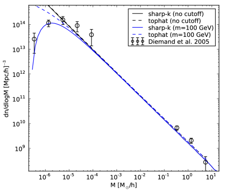
Fig. 8 presents the measured mass function from the simulations of Diemand et al. (2005) at $z=26$ as a function of halo mass. The black circles with error bars denote the estimates from the simulations: the three data points at the high mass end were derived from the lower resolution $L=3\,h^{-1}{\rm kpc}$ simulation, while the five points at lower masses are measurements from the high resolution zoom runs. The solid lines show the predictions from our sharp-$k$ space model mass function with ellipticity correction. The dashed ones show the results from the spherical tophat Sheth-Tormen model. Black curves correspond to the CDM model with no cutoff and blue corresponds to a scenario with 100 GeV neutralino cutoff. Note that the ellipticity correction has no effect here, since we are far away from the exponential tail of the mass function, and using the simple spherical mass assignment with the usual parameters $c=2.7$ and $q=1$ gives indistinguishable results.

The figure clearly shows that our sharp-$k$ mass function model agrees reasonably well with the simulation data and produces a turnover at about the right scale. Whilst this is an encouraging result, one should not over interpret its significance, owing to the poor statistics and the ‘by eye’ subtraction of artificial haloes. More detailed simulations would be necessary to see, for example, if the slightly steeper cutoff of the neutralino-CDM scenario, versus WDM, has a visible effect on the shape of the simulated mass function.

5.2 The complete CDM halo mass function

We now give a prediction of the redshift zero mass function for a neutralino-CDM scenario for the WMAP7 cosmological parameters. At wavenumbers well below the neutralino free-streaming cut-off scale we adopt the transfer function of Eisenstein & Hu (1998). This is a good choice for our purposes, since, whilst its accuracy is 2-3% for large scale $k$, it asymptotically approaches the exact analytical solution on small scales (above the cutoff). The neutralino cutoff scale depends on the mass of the neutralino and the temperature of kinetic decoupling (c.f. Eqs (9) and (11)). We shall take the mass of the neutralino to be 100 GeV. The actual decoupling temperature $T_{\rm dk}$, however is triggered by collisions with leptons and is model dependent. Bertschinger (2006) assumed $T_{\rm dk}=22.6$ MeV, while Green et al. (2005) found $T_{\rm dk}=33$ MeV, based on slightly different assumptions. In the following we adopt these two values as benchmarks, but note that other values are possible, depending on the specific parameters of supersymmetry.

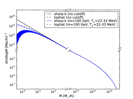
Fig. 9 shows our prediction for the mass function of dark matter haloes for a 100 GeV neutralino scenario as a function of halo mass. Our predictions cover the mass range from the most massive haloes $M\sim 10^{15}M_{\odot}$ until below the scale of one Earth mass at $M\sim 10^{-6}M_{\odot}$. For a better readability of the plot, we have excised the mass range between $10^{-3}M_{\odot}$ and $10^{12}M_{\odot}$, where the mass function is essentially a power law. The blue lines correspond to the model scenario with a 100 GeV cutoff, while the black lines are without cutoff. The shaded region enclosed by the dashed lines, denotes the standard spherical tophat mass function predictions spanned by the two benchmark decoupling temperatures $T_{\rm dk}=22.6$ MeV and $T_{\rm dk}=33$ MeV. The blue shaded region enclosed by the solid lines denotes our sharp-$k$ filter mass function predictions with ellipticity correction and the usual parameters $c_{\rm e}=2.0$ and $q=0.75$. Again, the simple spherical mass assignment with $c=2.7$ and $q=1$ gives very similar results.

The prediction of the neutralino-CDM mass function will be useful for estimations of the neutralino annihilation rate in the local universe.

Figure 9: Halo mass function of a 100 GeV neutralino WMAP7 cosmology at redshift zero. Solid line: sharp-$k$ filter; dashed line: Sheth-Tormen tophat filter. The actual half-mode mass scale of a 100 GeV neutralino depends on the temperature of kinetic decoupling which is model dependent. Here we have plotted the two benchmark values $T_{\rm dk}=22.6$ MeV and $T_{\rm dk}=33$ which delimit the blue shaded regions, where the dark blue region represents our new mass function model. The black lines corresponds to a model without cutoff.

6 Conclusions

In this paper we have developed a simple analytical model for the halo mass function in the presence of particle free streaming. This is an important task since numerical simulations produce artificial clumping at the scale corresponding to the power spectrum cutoff (half-mode scale) and it is currently impossible to numerically test structure formation below this scale. In a WDM scenario, however, it is crucial to understand the physics of structure formation below the half mode scale, since it is precisely on these scales where the alternative dark matter scenario can be either ruled out or confirmed.

Our method is based on the assumption that there is a direct mapping between the linear power spectrum and the final distribution of haloes, even in the presence of a power spectrum cutoff. In other words, this means that we assume the Extended Press-Schechter (EPS) approach to work for all cosmologies independent of the shape of the power spectrum. We note that this assumption remains unverified; it is for example imaginable that an EPS approach based on linear perturbation theory is not sufficient as soon as the power spectrum deviates from its quasi power-law shape, where EPS is much better verified against cosmological simulations. Instead, an approach with higher order perturbation could be necessary, or the EPS method could break down completely. On the longer term, it will be therefore indispensable to develop more accurate numerical methods capable of modelling the physics of gravitational structure formation on all scales without producing artificial clumping.

In the following, we list some key findings of this paper and discuss their range of applicability:

• In order to circumvent the problem of artificial clumping in our simulations we proposed an approximate method to subtract numerical artefacts from the halo mass function. The method is based on the observation that the mass function of artificial haloes has the form of a steep power-law that continues well above the mass range where artefacts dominate structure formation. This power-law is then simply subtracted from the measurements, a correction that makes the mass function turn over around the half-mode scale and decrease towards small masses, just as is expected from theoretical arguments. The power-law subtraction works surprisingly well at low redshift, where the corrected measurements of different box sizes are well-converged. At high redshift, however, the method seems to be less accurate as reflected by a poorer convergence between different box sizes, which appears to be caused in part because the artificial tail of the mass function is no longer such a clear power-law.

• We have constructed a simple model for the halo mass function based on a sharp-$k$ filter with constant $M\propto R^{3}$ mass assignment and a first crossing distribution from ellipsoidal collapse. It has the same number of free parameters as the standard Sheth-Tormen approach and gives accurate predictions for CDM as well as WDM scenarios at low redshift. At high redshift, however, as soon as the WDM half mode scale enters the exponential tail of the first crossing distribution, this simple method breaks down leading to an under-prediction of the halo abundance (Fig. 7, dotted lines). For a canonical 2 keV WDM candidate this happens at $z>5$.

• The breakdown of the simple model at high redshift comes from the fact that ellipsoidal patches are smoothed with a spherical window function, something that becomes important in WDM around the half-mode scale, where patches with high ellipticity cannot survive the free streaming. To improve upon this model, we include the effect of the patch ellipticity by taking the shortest ellipsoidal axes as the reference scale instead of the average radius that results when a spherical window function is applied. With this correction, our model yields an accurate mass function for CDM and WDM at all redshifts tested by our simulations.

• As a further application we used our model to predict the behaviour of the neutralino-CDM mass function, where the half-mode scale lies at an extremely small scale and where the power spectrum cutoff has a somewhat different form. A comparison to simulations from Diemand et al. (2005) shows reasonable agreement, but more precise simulations are necessary to test our mass function model in more detail.

The viability of the sharp-$k$ mass function at small scales well below the half mode scale still needs to be tested against simulations. This requires however a completely new numerical approach, since all common numerical schemes produce artefacts at the relevant scales, and this consists of a formidable scientific challenge.

Download Code

A code which calculates the sharp-$k$ mass function with or without ellipsoidal correction can be downloaded at: http://www.phys.susx.ac.uk/$\scriptstyle\sim$as721.

Appendix A Geometry of Patches

Patches around peaks of a Gaussian random field have an ellipsoidal form in the neighborhood around the peak. This observation was first done in the seminal paper of Bardeen et al. (1986), and it holds independently of the form of the underlying power spectrum. We will now summarize some of the results from Bardeen et al. (1986), and detail how the ellipsoidal axes are connected to the underlying power spectrum.

Around a local peak the density can be approximated by a Taylor expansion

$$\delta(r)=\delta(0)-\sum\lambda_{i}\frac{r_{i}^{2}}{2},\hskip 28.45274pt\lambda_{i}=\frac{\left[2\delta(0)-d\right]}{a_{i}^{2}},$$ (38)

where the constant density $d$ defines an ellipsoidal patch and connects the eigenvalues $\lambda_{i}$ of the tensor $\zeta_{ij}=\partial_{i}\partial_{j}\delta$ to the semi major axes of an ellipsoid $a_{i}$. The geometry of an ellipsoidal patch is characterized by the ellipticity and prolatness parameters

$$e=\frac{\lambda_{3}-\lambda_{1}}{2(\lambda_{1}+\lambda_{2}+\lambda_{3})},\hskip 28.45274ptp=\frac{\lambda_{3}-2\lambda_{2}+\lambda_{1}}{2(\lambda_{1}+\lambda_{2}+\lambda_{3})}.$$ (39)

From Eqs (38) and (39) it is now straight forward to derive the ratios of the ellipsoidal axes

$$\frac{a_{3}}{a_{1}}=\sqrt{\frac{1-3e+p}{1+3e+p}},\hskip 28.45274pt\frac{a_{3}}{a_{2}}=\sqrt{\frac{1-2p}{1+3e+p}},$$ (40)

that are used in the main text of this work. The ellipticity corrected mass function given by the Eqns (35), (36) and (37) can therefore be uniquely determined, provided we know the distribution of ellipticity and prolateness in our cosmology.

Bardeen et al. (1986) found analytical prescriptions of the probability distributions $P(e,p|x)$ as well as $P(x|\nu)$ (Eq. 7.6 and 7.5 in their paper), where $x=(\lambda_{1}+\lambda_{2}+\lambda_{3})/\sigma_{2}$ is the sum of the eigenvalues of the tensor $\zeta_{ij}$ divided by the second spectral moment. The spectral moments are defined as

$$\sigma^{2}_{j}(R)=\int\frac{{\rm d}^{3}{\bf k}}{(2\pi)^{3}}k^{2j}P_{\rm Lin}(k)W^{2}(kR),$$ (41)

and $\sigma_{0}$ is simply the variance defined in Eq. (15). The two probability distributions can be combined to obtain

$$P(e,p|\nu)=\int dxP(e,p|x)P(x|\nu),$$ (42)

which connects the ellipticity and prolateness parameters to the peak height $\nu$ and therefore the underlying power spectrum.

The distribution $P(x|\nu)$ is sharply peaked and has a maximum at

$$x_{m}=\gamma\nu+\frac{3(1-\gamma^{2})+(1.1-0.9\gamma^{4}){\rm e}^{-\gamma(1-\gamma^{2})(\gamma\nu/2)^{2}}}{[3(1-\gamma^{2})+0.45+(\gamma\nu/2)^{2}]^{1/2}+\gamma\nu/2}$$ (43)

where $\gamma=\sigma_{1}^{2}/(\sigma_{0}\sigma_{2})$ (Bardeen et al., 1986, Eq. 6.17). We ignore the distribution around $x_{\rm m}$ and just set $P(x|\nu)=\delta_{\rm D}(x-x_{\rm m})$, leading to to the simplified distribution $P(e,p|\nu)=P(e,p|x_{\rm m})$.

Bardeen et al. (1986) found that $P(e,p|x_{\rm m})$ is approximately Gaussian (for large x) and has a maximum at

$$e_{\rm m}=\frac{1}{(5x_{\rm m}^{2}+6)^{1/2}},\hskip 28.45274ptp_{\rm m}=\frac{30}{(5x_{\rm m}^{2}+6)^{2}}.$$ (44)

It is now straight forward to derive average axes ratios by substituting Eq. (44) into Eq. (40). The result of this calculation is given in Fig. 7 (see main text for more information).

Appendix B Subtraction of artificial haloes at higher redshifts

In the main text we discussed the power-law subtraction of the artificial haloes in detail, and we plotted the utilised power-law fit in Fig. 4. Here we will give the same plots for the correction of halo abundance at higher redshift (Fig. 10).

Figure 10: Correction of WDM halo abundance at higher redshifts. From top to bottom: $z=1.1$, $z=2.4$ and $z=4.4$. From left to right: WDM with $m_{\rm WDM}=0.25\,{\rm keV}$, WDM with $m_{\rm WDM}=0.5\,{\rm keV}$ and WDM with $m_{\rm WDM}=1.0\,{\rm keV}$. The CDM measurements have been added to every panel for comparison. The faint symbols correspond to the original mass function, the bold symbols correspond to the corrected mass function. The grey lines are the power-laws which are used for the subtraction. The fitting is done over the yellow symbols.

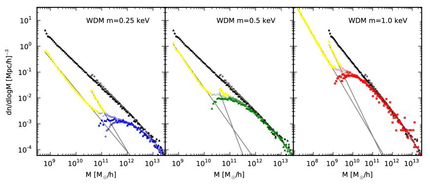
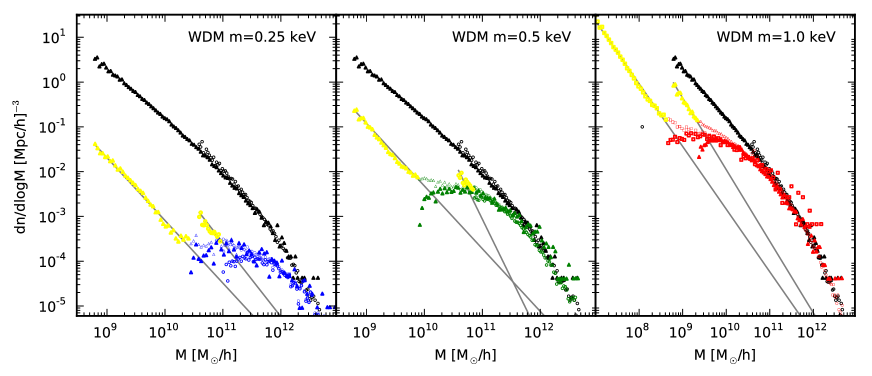
As a matter of fact, the higher the redshift the less the upturn has the shape of a single power-law. This makes it more difficult to do a proper fit and leaves space for ambiguity in the model building.

References

- Anderhalden & Diemand (2013) Anderhalden, D., Diemand, J., Bertone, G., Macciò, A. V., & Schneider A. 2012, Journal of Cosmology and Astro-Particle Physics, 10 047A
- Anderhalden et al. (2012) Anderhalden, D. & Diemand, J. 2013, arXiv:1302.0003
- Anderhalden et al. (2013) Anderhalden, D., Schneider A., Macciò, A. V., Diemand, J., & Bertone, G. 2012, arXiv:1212.2967
- Bardeen et al. (1986) Bardeen, J. M., Bond, J. R., Kaiser, N., & Szalay, A. S. 1986, ApJ, 304, 15
- Barkana et al. (2001) Barkana, R., Haiman, Z., & Ostriker, J. P. 2001, ApJ, 558, 482
- Benson et al. (2012) Benson, A. J. et al. 2013, MNRAS, 428,1774B
- Bertschinger (2006) Bertschinger, E. 2006, Phys. Rev. D, 74, 063509, L1
- Bhattacharya et al. (2011) Bhattacharya, S., Heitmann, K., White, M., Lukić, Z., Wagner, C. & Habib, S. 2011, ApJ, 732, 112B
- Bode et al. (2001) Bode, P., Ostriker, J. P., & Turok, N. 2001, ApJ, 556, 93
- Bond et al. (1991) Bond, J. R., Cole, S., Efstathiou, G., & Kaiser, N. 1991, ApJ, 379, 440
- Bond & Szalay (1983) Bond, J. R. & Szalay, A. S. 1983, ApJ, 274, 443
- Colombi et al. (1996) Colombi, S., Dodelson, S., & Widrow, L. M. 1996, ApJ, 458, 1
- Crocce et al. (2006) Crocce, M., Pueblas, S., & Scoccimarro, R. 2006, MNRAS, 373, 369
- Davis et al. (1985) Davis, M., Efstathiou, G., Frenk, C. S., & White, S. D. M. 1985, ApJ, 292, 371
- Diemand et al. (2005) Diemand, J., Moore, B., & Stadel, J. 2005, Nature, 433, 389
- Dodelson & Widrow (1994) Dodelson, S. & Widrow, L. M. 1994, Physical Review Letters, 72, 17
- Eisenstein & Hu (1998) Eisenstein, D. J. & Hu, W. 1998, ApJ, 496, 605
- Eke et al. (1996) Eke, V. R., Cole, S., & Frenk, C. S. 1996, MNRAS, 282, 263
- Elahi et al. (2009) Elahi, P. J., Thacker, R. J., Widrow, L. M., & Scannapieco, KE. 2009, MNRAS395, 1950
- Goerdt et al. (2007) Goerdt, T., Gnedin, O. Y., Moore, B., Diemand, J., Stadel, J. 2007, MNRAS, 375, 191
- Green et al. (2004) Green, A. M., Hofmann, S., & Schwartz, D. J., 2004, MNRAS, 353, 23
- Green et al. (2005) Green, A. M., Hofmann, S., & Schwartz, D. J., 2005, Journal of Cosmology and Astro-Particle Physics, 08, 003
- Hahn et al. (2012) Hahn, O., Abel, T., & Kaehler, R. 2012, arXiv:1210.6652
- Hofmann et al. (2001) Hofmann, S., Schwartz, D. J., & Stöcker, H. 2001, Phys. Rev. D, 64, 083507
- Ishiyama et al. (2010) Ishiyama, T., Makino, J., & Ebisuzaki, T. 2010, ApJ, 723L, 196I
- Jungman et al. (1996) Jungman, G., Kamionkowski, M., & Griest, K. 1996, Phys. Rep. , 267, 195
- Kamionkowski & Koushiappas (2008) Kamionkowski & M., Koushiappas, S. M. 2008, Phys. Rev. D, 77, 3509
- Komatsu et al. (2011) Komatsu, E., Smith, K. M., Dunkley, J., & The WMAP Team. 2011, ApJS, 192, 18
- Koushiappas (2009) Koushiappas, S. M. 2009, NJPH, 11, 512K
- Lacey & Cole (1993) Lacey, C. & Cole, S. 1993, MNRAS, 262, 627
- Lahav et al. (1991) Lahav, O., Lilje, P. B., Primack, J. R., & Rees, M. J. 1991, MNRAS, 251, 128
- Lewis et al. (2000) Lewis, A., Challinor, A., & Lasenby, A. 2000, Astrophys. J., 538, 473
- Lovell et al. (2011) Lovell, M., Eke, V., Frenk, C., Gao, L., Jenkins, A., Theuns, T., Wang, J., Boyarsky, A., & Ruchayskiy, O. 2011, ArXiv e-prints
- Maggiore & Riotto (2010) Maggiore, M. & Riotto, A. 2010, ApJ, 711 907M
- Maccio et al. (2012) Macciò, A. V., Paduroiu, S., Anderhalden, D., Schneider, A., & Moore, B. 2012, MNRAS, 424, 1105M
- Maccio et al. (2012) Macciò, A. V., Ruchayskiy, O., Boyarsky, A., & Mu oz-Cuartas, J. C. 2012, MNRAS, 428, 882M
- Musso & Sheth (2012) Musso, M. & Sheth, R. 2012, MNRAS, 423L, 102M
- Peebles (1982) Peebles, P. J. E. 1982, ApJL, 263, L1
- Press & Schechter (1974) Press, W. H. & Schechter, P. 1974, ApJ, 187, 425
- Reed et al. (2007) Reed, D. S., Bower, R., Frenk, C. S., Jenkins, A., & Theuns, T. 2007, MNRAS, 374, 2
- Scoccimarro (1998) Scoccimarro, R. 1998, MNRAS, 299, 1097
- Schneider et al. (2010) Schneider, A., Krauss, L. M., Moore, B., 2010, PRD, 82, 063525
- Schneider et al. (2012) Schneider, A., Smith, R. E., Macciò, A. V., Moore, B., 2012, MNRAS, 424, 684S
- Shao et al. (2013) Shao, S., Gao, L., Theuns, T., & Frenk, C. S 2013, MNRAS, tmp, 736
- Sheth & Tormen (1999) Sheth, R. K. & Tormen, G. 1999, MNRAS, 308, 119
- Smith & Markovic (2011) Smith, R. E. & Markovic, K. 2011, Phys. Rev. D, 84, 063507
- Smith et al. (2003) Smith, R. E., Peacock, J. A., Jenkins, A., White, S. D. M., Frenk, C. S., Pearce, F. R., Thomas, P. A., Efstathiou, G. & Couchman, H. M. P. 2007, MNRAS, 341, 1311
- Spergel et al. (2003) Spergel, D. N. et al. 2003, ApJ, 148, 175
- Springel (2005) Springel, V. 2005, MNRAS, 364, 1105
- Stadel (2001) Stadel, J. G. 2001, PhD thesis, AA(UNIVERSITY OF WASHINGTON)
- Viel et al. (2005) Viel, M., Lesgourgues, J., Haehnelt, M. G., Matarrese, S., & Riotto, A. 2005, PRD, 71, 063534
- Villaescusa-Navarro & Dalal (2011) Villaescusa-Navarro, F. & Dalal, N. 2011, Journal of Cosmology and Astro-Particle Physics, 3, 24
- Vogelsberger et al. (2012) Vogelsberger, M., Zavala, J., & Loeb, A. 2012, MNRAS, 423, 3740
- Wang & White (2007) Wang, J. & White, S. D. M. 2007, MNRAS, 380, 93
- Watson et al. (2012) Watson, W. A., Iliev, I. T., D’Aloisio, A., Knebe, A., Shapiro, P. R., & Yepes, G. 2012, arXiv:1212.0095