Fermionic vacuum polarization by a cosmic string
in anti-de Sitter spacetime

Abstract

In this paper we investigate the fermionic condensate (FC) and the vacuum expectation value (VEV) of the energy-momentum tensor, associated with a massive fermionic field, induced by the presence of a cosmic string in the anti-de Sitter (AdS) spacetime. In order to develop this analysis we construct the complete set of normalized eigenfunctions in the corresponding spacetime. We consider a special case of boundary conditions on the AdS boundary, when the MIT bag boundary condition is imposed on the field operator at a finite distance from the boundary, which is then taken to zero. The FC and the VEV of the energy-momentum tensor are decomposed into the pure AdS and string-induced parts. Because the analysis of one-loop quantum effects in the AdS spacetime has been developed in the literature, here we are mainly interested to investigate the influence of the cosmic string on the VEVs. The string-induced part in the VEV of the energy-momentum tensor is diagonal and the axial and radial stresses are equal to the energy density. For points near the string, the effects of the curvature are subdominant and to leading order, the VEVs coincide with the corresponding VEVs for the cosmic string in Minkowski bulk. At large proper distances from the string, the decay of the VEVs show a power-law dependence of the distance for both massless and massive fields. This is in contrast to the case of Minkowski bulk where, for a massive field, the string-induced parts decay exponentially.

PACS numbers: 03.70.+k, 98.80.Cq, 11.27.+d

1 Introduction

The nontrivial properties of the vacuum are among the most important consequences in quantum field theory. These properties depend on both the local and global geometrical characteristics of the background spacetime. In particular, the boundary conditions imposed on a quantum field in spaces with non-trivial topology modify the spectrum for zero-point fluctuations which give rise to change in the vacuum expectation values (VEVs) for physical observables. A well known example of this kind of phenomenon is the topological Casimir effect. The explicit dependence of the physical characteristics of the vacuum on the geometrical properties of the bulk, can be found for highly-symmetric backgrounds only. In this paper we consider an exactly solvable problem for the fermionic vacuum polarization by a cosmic string in the background of anti-de Sitter (AdS) spacetime.

The importance of AdS spacetime as a background geometry in quantum field theory is motivated by several reasons. The early interest was related to principal questions of the quantization of fields on curved backgrounds. The lack of global hyperbolicity and the presence of both regular and irregular modes give rise to a number of new phenomena which have no analogs in quantum field theory on the Minkowski bulk. These phenomena have been discussed by several authors considering both scalar [1]-[3] and spinor [4]-[8] fields. The importance of this research increased by the natural appearance of AdS spacetime as a ground state in supergravity and Kaluza-Klein theories. The AdS geometry plays a crucial role in two exciting developments in theoretical physics of the past decade such as the AdS/CFT correspondence and the braneworld scenario with large extra dimensions. The AdS/CFT correspondence (for a review see [9]), represents a realization of the holographic principle and relates string theories or supergravity in AdS bulk with a conformal field theory living on its boundary. The braneworld scenario offers a new perspective on the hierarchy problem between the gravitational and electroweak mass scales (for reviews on braneworld gravity and cosmology see [10]). The main idea to resolve the large hierarchy is that the small coupling of 4-dimensional gravity is generated by the large physical volume of extra dimensions.

In the framework of grand unified theories, different types of topological defects may have been created in the early universe as a consequence of the vacuum phase transition [11, 12]. Among them cosmic strings are of special interest. Although recent observations data on the cosmic microwave background have ruled out cosmic strings as the primary source for primordial density perturbation, they are still candidate for the generation of a number of interesting physical effects such as gamma ray burst [13], gravitational waves [14] and high energy cosmic rays [15]. Recently, cosmic strings have attracted renewed interest partly because a variant of their formation mechanism is proposed in the framework of brane inflation [16]-[18].

The geometry of a cosmic string in the background of AdS spacetime has been considered in [39, 40]. It has been shown that, similar to the case of Minkowskian bulk, at distances from the string larger than its core radius, the gravitational effects of the string can be described by a planar angle deficit in the AdS line-element. The corresponding non-trivial topology induces vacuum polarization effects for quantum fields. These effects are well-investigated for the geometry of a cosmic string in Minkowski spacetime for scalar [19]-[24], fermionic [25]-[29] and vector quantum fields [30]-[32]. Recently the corresponding results have been generalized for cosmic string in curved spacetime. Specifically, one-loop quantum effects have been considered for a massless scalar field in Schwarzschild spacetime [33], for massive scalar [34] and fermionic [35] fields in de Sitter spacetime, and also for a massive scalar field in AdS spacetime [36]. In the present paper, we continue along similar line of investigation, analyzing the fermionic vacuum polarization effects associated with a massive Dirac spinor field in a four-dimensional AdS spacetime in the presence of a cosmic string. Among the most important local physical characteristics of the fermionic vacuum are the fermionic condensate and the VEV of the energy-momentum tensor. The fermionic condensate plays an important role in the models of dynamical breaking of chiral symmetry, whereas the VEV of the energy-momentum tensor acts as the source of gravity in the quasiclassical Einstein equations.

This paper is organized as follows: In section 2 we present the background geometry associated with the spacetime under consideration and construct the complete set of positive- and negative-energy fermionic wave-functions. In section 3 we calculate the fermion condensate by using the mode-summation method. In this evaluation the contribution induced by the cosmic string is separately analyzed and its behavior in the asymptotic regions of the parameters is investigated. The analysis of the VEV of the energy-momentum tensor is considered in section 4. There, the contribution induced by the cosmic string is also investigated. Finally, the main results of the paper are summarized in section 5. In appendix we show that the mode functions used in the main text are obtained when the MIT bag boundary condition is imposed at a finite distance from the AdS boundary, which is then taken to zero. Throughout of the paper we shall use the units $\hbar=c=G=1$.

2 Fermionic wave-functions

The main objective of this section is to obtain the complete set of fermionic mode-functions in a four-dimensional AdS spacetime in presence of a cosmic string. This set is needed in the calculation of vacuum polarization effects by using the mode-summation approach.

In cylindrical coordinates, considering a static string along the $y$-axis, the geometry associated with a cosmic string in a four-dimensional AdS spacetime is given by the following line element:

$$ds^{2}=e^{-2y/a}\left(-dt^{2}+dr^{2}+r^{2}d\phi^{2}\right)+dy^{2}\ ,$$ (1)

where $r\geq 0$ and $\phi\in[0,\ 2\pi/q]$ define the coordinates on the conical subspace, $(t,\ y)\in(-\infty,\ \infty)$. The points $(r,\ \phi,\ z)$ and $(r,\phi+2\pi/q,z)$ are to be identified, and the parameter $a$ is related with the cosmological constant and Ricci scalar for AdS spacetime by the formulas

$$\Lambda=-3a^{-2},\ R=-12a^{-2}\ .$$ (2)

The parameter $q$, bigger than unity, codifies the presence of the cosmic string.

By using the Poincaré coordinate defined as $z=ae^{y/a}$, the line element above is presented in the form conformally related to the line element associated with a cosmic string in Minkowski spacetime:

$$ds^{2}=(a/z)^{2}\left(-dt^{2}+dr^{2}+r^{2}d\phi^{2}+dz^{2}\right)\ .$$ (3)

For this new coordinate one has $z\in[0,\ \infty)$. The hypersurfaces $z=0$ and $z=\infty$ correspond to the AdS boundary and horizon, respectively.

Although the line element for an infinite straight cosmic string in the background of Minkowski spacetime, which corresponds to the expression inside the parentheses in (3), has been derived in [37] by making use of weak-field approximation, the validity of this solution has been extended beyond the linear perturbation theory by several authors [38]. In this case the parameter $q$ need not to be close to the unity. The metric tensor corresponding to the line element (1) is an exact solution of the Einstein equation in the presence of a negative cosmological constant and the string [39, 40], for arbitrary values of $q$.

The quantum motion of a massive spinor field on curved spacetime is governed by the Dirac equation

$$i\gamma^{\mu}\nabla_{\mu}\psi-m\psi=0\ ,\;\nabla_{\mu}=\partial_{\mu}+\Gamma_{\mu}\ ,$$ (4)

where $\gamma^{\mu}$ are the Dirac matrices in curved spacetime and $\Gamma_{\mu}$ is the spin connection. They are given in terms of the flat spacetime Dirac matrices, $\gamma^{(a)}$, by the relations,

$$\gamma^{\mu}=e_{(a)}^{\mu}\gamma^{(a)}\ ,\ \Gamma_{\mu}=-\frac{1}{4}\gamma^{(a)}\gamma^{(b)}e_{(a)}^{\nu}e_{(b)\nu;\mu}\ ,$$ (5)

where the semicolon means the standard covariant derivative for vector fields. In (5), $e_{(a)}^{\mu}$ is the tetrad basis satisfying the relation $e_{(a)}^{\mu}e_{(b)}^{\nu}\eta^{ab}=g^{\mu\nu}$, with $\eta^{ab}$ being the Minkowski spacetime metric tensor.

In order to simplify the obtainment of the fermionic wave-functions in the geometry under consideration, we shall use for the flat space Dirac matrices the representation which is obtained from the matrices given in [41] multiplied on the left by $i\gamma^{(5)}$ matrix. In this representation one has

$$\gamma^{(0)}=-i\left(\begin{array}[]{cc}0&1\\ -1&0\end{array}\right)\ ,\ \gamma^{(a)}=-i\left(\begin{array}[]{cc}\sigma_{a}&0\\ 0&-\sigma_{a}\end{array}\right)\ ,\ a=1,2,3\ ,$$ (6)

with $\sigma_{1},\sigma_{2},\sigma_{3}$ being the Pauli matrices. It can be verified that the above matrices obey the Clifford algebra, $\{\gamma^{(a)},\ \gamma^{(b)}\}=-2\eta^{ab}$.

The basis of tetrads corresponding to the line element (3) can be taken in the form

$$e_{(a)}^{\mu}=\frac{z}{a}\left(\begin{array}[]{cccc}1&0&0&0\\ 0&\cos(q\phi)&-\sin(q\phi)/r&0\\ 0&\sin(q\phi)&\cos(q\phi)/r&0\\ 0&0&0&1\end{array}\right)\ .$$ (7)

With this choice, the curved space gamma matrices read:

$$\gamma^{0}=\frac{z}{a}\gamma^{(0)}\ ,\ \gamma^{i}=-i\frac{z}{a}\left(\begin{array}[]{cc}\sigma^{i}&0\\ 0&-\sigma^{i}\end{array}\right)\ ,$$ (8)

where the index $i$ corresponds to the coordinates $r,\ \phi,\ z$. The $2\times 2$ matrices in (8) are given by

$$\sigma^{r}=\left(\begin{array}[]{cc}0&e^{-iq\phi}\\ e^{iq\phi}&0\end{array}\right),\ \sigma^{\phi}=-\frac{i}{r}\left(\begin{array}[]{cc}0&e^{-iq\phi}\\ -e^{iq\phi}&0\end{array}\right),\ \ \sigma^{z}=\left(\begin{array}[]{cc}1&0\\ 0&-1\end{array}\right).$$ (9)

For the spin connection components we obtain:

$$\Gamma_{\mu}=-\frac{1}{2a}\gamma^{(3)}\gamma_{\mu}+\frac{(1-q)}{2}\gamma^{(1)}\gamma^{(2)}\delta_{\mu}^{\phi}\ ,\ \Gamma_{z}=0\ .$$ (10)

This leads to the following expression for the combination appearing in the Dirac equation (4):

$$\gamma^{\mu}\Gamma_{\mu}=-\frac{3}{2z}\gamma^{z}+\frac{1-q}{2r}\gamma^{r}\ .$$ (11)

Taking the time dependence for the positive-energy four-component spinor in the form $e^{-iEt}$, and decomposing it into upper and lower two-component spinors denoted by $\varphi$ and $\chi$, respectively, the Dirac equation can be written as shown below:

$$\left(\sigma^{l}\partial_{l}-\frac{3}{2z}\sigma^{z}+\frac{1-q}{2r}\sigma^{r}-\frac{ma}{z}\right)\varphi-iE\chi = 0\ ,$$

$$\left(\sigma^{l}\partial_{l}-\frac{3}{2z}\sigma^{z}+\frac{1-q}{2r}\sigma^{r}+\frac{ma}{z}\right)\chi-iE\varphi = 0\ .$$ (12)

Substituting the spinor $\chi$ from the first equation into the second one, we obtain a second order differential equation for $\varphi$:

$$\left[\partial_{r}^{2}+\frac{1}{r}\partial_{r}-i\frac{1-q}{r^{2}}\sigma^{3}\partial_{\phi}+\frac{1}{r^{2}}\partial_{\phi}^{2}+\partial_{z}^{2}-\frac{3}{z}\partial_{z}\right.$$

$$\left.-\frac{(1-q)^{2}}{4r^{2}}+\frac{15-4m^{2}a^{2}}{4z^{2}}+\frac{ma}{z^{2}}\sigma^{z}+E^{2}\right]\varphi=0\ .$$ (13)

Because the above equation has a diagonal form, we can obtain two second order differential equations decomposing the two-component spinor $\varphi$ into the upper and lower components, denoted by $\varphi_{1}$ and $\varphi_{2}$, respectively. Taking these functions in the form $\varphi_{l}(x)=e^{iqn_{l}\phi}R_{l}(r)Z_{l}(z)$, with $l=1,2$, we can see that the normalizable solution for the radial function is expressed in terms of the Bessel function of the first kind, $R_{l}(r)=J_{\beta_{l}}(\lambda r)$, with the order,

$$\beta_{l}=|qn_{l}-(-1)^{l}(q-1)/2|,$$ (14)

where $n_{l}=0,\pm 1,\pm 2,\ ...$. As to the function $Z_{l}(z)$, the general solution is given in terms of a linear combination of the functions $z^{2}J_{\nu_{l}}(kz)$ and $z^{2}Y_{\nu_{l}}(kz)$, where $Y_{\nu}(x)$ is the Neumann function and

$$\nu_{l}=ma+(-1)^{l}/2\ .$$ (15)

For $ma\geq 1/2$ the part with the Neumann function is excluded by the normalizability condition of the mode functions and the solution for the function $Z_{l}(z)$ reads:

$$Z_{l}(z)=z^{2}J_{\nu_{l}}(kz)\ .$$ (16)

As to the energy, it is given by

$$E=\sqrt{\lambda^{2}+k^{2}}\ .$$ (17)

For $ma<1/2$, the modes with the Neumann function are normalizable as well. In this case, in order to specify uniquely the mode functions, an additional boundary condition is required on the AdS boundary $z=0$. Here, for the case $ma<1/2$, we consider a special case of boundary conditions at the AdS boundary, when the MIT bag boundary condition is imposed at a finite distance from the boundary, $z=\delta$, which is then taken to zero, $\delta\rightarrow 0$ (FC and the VEV of the energy-momentum tensor for the geometry of two flat boundaries in AdS bulk with the bag boundary conditions have been recently discussed in [8]). In Appendix we show that this procedure leads to the choice of the mode functions in the form (16) and ensures the zero current of fermions through the AdS boundary. Note that the boundary condition we have used also excludes the normalizable modes with $Z_{l}(z)=z^{2}K_{\nu_{l}}(z\sqrt{\lambda^{2}-E^{2}})$, $\lambda>E$, where $K_{\nu}(x)$ is the Macdonald function.

Finally, we can write the upper two-component spinor in the form

$$\varphi_{l}=C_{l}z^{2}J_{\beta_{l}}(\lambda r)J_{\nu_{l}}(kz)e^{iqn_{l}\phi}\ .$$ (18)

Having the upper component spinor, the lower one is obtained by using the first equation of (12). After some intermediate steps we find:

$$\chi_{1} = B_{1}e^{iqn_{1}\phi}J_{\beta_{1}}(\lambda r)z^{2}J_{\nu_{2}}(kz)\ ,$$

$$\chi_{2} = B_{2}e^{iqn_{2}\phi}J_{\beta_{2}}(\lambda r)z^{2}J_{\nu_{1}}(kz)\ ,$$ (19)

with the relations

$$n_{2}=n_{1}+1\ ,\ \beta_{2}=\beta_{1}+\epsilon_{n_{1}}\ ,$$ (20)

where $\epsilon_{n}=1$ for $n\geq 0$ and $\epsilon_{n}=-1$ for $n<0$. The coefficients $B_{1,2}$ in (19) are given by the expressions

$$B_{1}=\frac{i}{E}\left(kC_{1}-\epsilon_{n_{1}}\lambda C_{2}\right)\ ,\ B_{2}=\frac{i}{E}\left(\epsilon_{n_{1}}\lambda C_{1}+kC_{2}\right)\ .$$ (21)

We can see that the fermionic wave-functions defined with the upper and lower components given by relations (18) and (19), respectively, are eigenfunctions of the projection of the total momentum along the direction of the cosmic string:

$$\widehat{J}_{z}\psi=\left(-i\partial_{\phi}+\frac{q}{2}\Sigma^{z}\right)\psi=qj\psi\ ,\ \Sigma^{z}=\left(\begin{array}[]{cc}\sigma^{z}&0\\ 0&\sigma^{z}\end{array}\right)\ ,$$ (22)

where

$$j=n_{1}+1/2\ ,\ j=\pm 1/2,\pm 3/2\ ,\ldots\ .$$ (23)

The fermionic wave-functions we have derived contain four coefficients and there are two equations relating them. The normalization condition on the functions provides an extra equation. Consequently, one of the coefficients remains arbitrary. In order to determine this coefficient some additional condition should be imposed on the coefficients. The necessity for this condition is related to the fact that the quantum numbers $(\lambda,k,j)$ do not specify the fermionic wave-function uniquely and some additional quantum number is required.

In order to specify the second constant we impose the condition

$$C_{1}/B_{1}=-C_{2}/B_{2}\ .$$ (24)

By taking into account (21) we get the relations:

$$C_{2}=-\epsilon_{n_{1}}b_{s}^{(+)}C_{1}\ ,\ B_{1}=isC_{1}\ ,\ B_{2}=i\epsilon_{n_{1}}sb_{s}^{(+)}C_{1}\ ,$$ (25)

where and in what follows

$$b_{s}^{(\pm)}=\frac{sE\mp k}{\lambda}\ ,\ \ s=\pm 1\ .$$ (26)

Note that one has $b_{s}^{(+)}b_{s}^{(-)}=1$. With the condition (24), the fermionic mode functions are uniquely specified by the set $\sigma=(\lambda,k,j,s)$. Instead of (24) we could impose another condition. The only restriction is that the resulting wave-functions should form a complete set. For example, the condition similar to (24) with the opposite sign of the right-hand side gives another set of wave-functions. Different conditions give the same two-point functions and, as a result, the same VEVs for physical observables.

On the basis of the discussion above, for the positive-energy fermionic wave-function we can write the following expression:

$$\psi_{\sigma}^{(+)}(x)=C_{\sigma}^{(+)}e^{-iEt}z^{2}\left(\begin{array}[]{c}J_{\beta_{1}}(\lambda r)J_{\nu_{1}}(kz)\\ -\epsilon_{j}b_{s}^{(+)}J_{\beta_{2}}(\lambda r)J_{\nu_{2}}(kz)e^{iq\phi}\\ isJ_{\beta_{1}}(\lambda r)J_{\nu_{2}}(kz)\\ i\epsilon_{j}sb_{s}^{(+)}J_{\beta_{2}}(\lambda r)J_{\nu_{1}}(kz)e^{iq\phi}\end{array}\right)e^{iq(j-1/2)\phi}\ ,$$ (27)

where the order of the Bessel functions are defined in terms of $j$ as:

$$\beta_{l}=|qj+(-1)^{l}/2|=q|j|+(-1)^{l}\epsilon_{j}/2\ .$$ (28)

Notice that $\epsilon_{j}=\epsilon_{n_{1}}$.

The coefficient $C_{\sigma}^{(+)}$ in (27) is determined from the normalization condition

$$\int d^{3}x\sqrt{\gamma}\ (\psi_{\sigma}^{(+)})^{\dagger}\psi_{\sigma^{\prime}}^{(+)}=\delta_{\sigma\sigma^{\prime}}\ ,$$ (29)

where $\gamma$ is the determinant of the spatial metric. The delta symbol on the right-hand side is understood as the Dirac delta function for continuous quantum numbers $(\lambda,\ k)$ and the Kronecker delta for discrete ones $(j,s)$. Substituting the eigenspinors (27) into (29) and using the value of the standard integral involving the products of the Bessel functions [42], we find

$$|C_{\sigma}^{(+)}|^{2}=\frac{sq\lambda^{2}k}{8\pi a^{3}Eb_{s}^{(+)}}\ .$$ (30)

In the discussion above, as solutions of the equations for the radial parts of the mode functions we have taken the Bessel functions $J_{\beta_{l}}(\lambda r)$, $l=1,2$. This choice corresponds to the modes regular on the string. In addition, we could consider the irregular modes with the Neumann functions $Y_{\beta_{l}}(\lambda r)$. For these modes to be normalizable the integral $\int_{0}^{\infty}dr\,rY_{\beta_{l}}(\lambda r)Y_{\beta_{l}}(\lambda^{\prime}r)$ should converge at the lower limit of the integration for both $l=1$ and $l=2$. From the condition of the convergence for $l=2$ one gets the constraint $q|j|<1/2$, which cannot be satisfied for $q\geqslant 1$. Hence, in the problem under consideration there are no normalizable modes irregular on the string. Note that, irregular normalizable modes are possible in the presence of a magnetic flux running along the axis of the string.

The negative-energy fermionic wave-function, can be obtained from the positive-energy function by the charge conjugate matrix. Following the general procedure given in [41], the charge conjugation matrix, $\mathcal{C}$, must obey the relation ${\mathcal{C}}(\gamma^{(a)})^{\ast}{\mathcal{C}}^{-1}=-\gamma^{(a)}$, with $(\gamma^{(a)})^{\ast}$ denoting the complex conjugate. In the representation used by us for the Dirac matrices, all but $\gamma^{(2)}$ matrix are complex ones; so $\mathcal{C}$ must anti-commute with $\gamma^{(2)}$ and commute with the others. Up to an overall phase, a particular choice for this matrix is,

$${\mathcal{C}}=\gamma^{(5)}\gamma^{(2)}=i\left(\begin{array}[]{cc}0&\sigma_{2}\\ -\sigma_{2}&0\end{array}\right)={\mathcal{C}}^{-1}\ .$$

The negative-energy wave-function can be given by $\psi_{\sigma}^{(-)}(x)={\mathcal{C}}(\psi_{\sigma}^{(+)}(x))^{\ast}$. The final result is

$$\psi_{\sigma}^{(-)}(x)=C_{\sigma}^{(-)}e^{iEt}z^{2}\left(\begin{array}[]{c}J_{\beta_{2}}(\lambda r)J_{\nu_{1}}(kz)\\ -\epsilon_{j}b_{s}^{(-)}J_{\beta_{1}}(\lambda r)J_{\nu_{2}}(kz)e^{iq\phi}\\ isJ_{\beta_{2}}(\lambda r)J_{\nu_{2}}(kz)\\ i\epsilon_{j}sb_{s}^{(-)}J_{\beta_{1}}(\lambda r)J_{\nu_{1}}(kz)e^{iq\phi}\end{array}\right)e^{-iq(j+1/2)\phi}\ ,$$ (31)

with the same notations as in (27), and $C_{\sigma}^{(-)}=-i\epsilon_{j}sb_{s}^{(+)}(C_{\sigma}^{(+)})^{\ast}$. The modulus of the normalization constant $C_{\sigma}^{(-)}$ can also be evaluated by using the normalization condition similar to the one for the positive-energy wave-function, Eq. (29). Its value reads,

$$|C_{\sigma}^{(-)}|^{2}=\frac{sq\lambda^{2}k}{8\pi a^{3}Eb_{s}^{(-)}}\ .$$ (32)

The wave-functions obtained in this section can be used for the investigation of various quantum effects around the cosmic string involving electrons and positrons. In what follows we use these functions for the evaluation of the fermionic condensate and the VEV of the energy-momentum tensor.

3 Fermionic condensate

Having obtained the normalized positive- and negative-energy fermionic wave-functions, we are able to calculate the fermionic condensate (FC), $\langle 0|\bar{\psi}\psi|0\rangle$, where $|0\rangle$ is the vacuum state in the AdS spacetime in the presence of a cosmic string, and $\bar{\psi}_{\sigma}^{(-)}=\psi_{\sigma}^{(-)\dagger}\gamma^{(0)}$ is the Dirac adjoint. Expanding the field operator in terms of the complete set $\{\psi_{\sigma}^{(-)},\ \psi_{\sigma}^{(+)}\}$, the following formula for the FC is obtained:

$$\langle 0|\bar{\psi}\psi|0\rangle=\sum_{\sigma}\bar{\psi}_{\sigma}^{(-)}\psi_{\sigma}^{(-)}\ ,$$ (33)

where we use the compact notation defined below,

$$\sum_{\sigma}=\int_{0}^{\infty}\ d\lambda\ \int_{0}^{\infty}\ dk\ \sum_{s=\pm 1}\sum_{j=\pm 1/2,\cdots}\ .$$ (34)

Substituting the eigenspinor (31) into (33), we obtain

$$\langle 0|\bar{\psi}\psi|0\rangle = \frac{qz^{4}}{4\pi a^{3}}\sum_{\sigma}\frac{\lambda^{2}\ k}{E}J_{\nu_{1}}(kz)J_{\nu_{2}}(kz)$$ (35)

$$\times\left[b_{s}^{(+)}J_{\beta_{2}}^{2}(\lambda r)-b_{s}^{(-)}J_{\beta_{1}}^{2}(\lambda r)\right]\ .$$

The fermionic condensate given by (35) is divergent and some regularization procedure is necessary. We shall assume that a cutoff function is introduced in the above formula without explicitly writing it. As we shall see, the explicit form of this function is not relevant for the further discussion

The sum over the total angular quantum number $j$ for the corresponding Bessel functions provide the same expression for $l=1$ and $l=2$:

$$\sum_{j=\pm 1/2,\cdots}J_{\beta_{l}}^{2}(\lambda r)=\sum_{j}\left[J_{qj-1/2}^{2}(\lambda r)+J_{qj+1/2}^{2}(\lambda r)\right]\ .$$ (36)

Here and in what follows, we use the notation

$$\sum_{j}=\sum_{j=1/2,\cdots}\ .$$ (37)

Now it is possible to develop the summation over the quantum number $s$. The result is expressed as,

$$\langle 0|\bar{\psi}\psi|0\rangle=-\frac{q\ z^{4}}{\pi a^{3}}\int_{0}^{\infty}d\lambda\int_{0}^{\infty}dk\frac{\lambda\ k^{2}}{E}J_{\nu_{1}}(kz)J_{\nu_{2}}(kz)\sum_{j}\left[J_{qj+1/2}^{2}(\lambda r)+J_{qj-1/2}^{2}(\lambda r)\right]\ .$$ (38)

In order to provide a more workable expression for the FC, we use the identity

$$\frac{1}{E}=\frac{2}{\sqrt{\pi}}\int_{0}^{\infty}ds\ e^{-(\lambda^{2}+k^{2})s^{2}}\ .$$ (39)

Substituting this identity into (38), it is possible to develop the integrations over the variables $\lambda$ and $k$ with the help of formula from [42]. Although the orders of the Bessel functions associated with the $z$-variable are different, the integral over $k$ is evaluated because $\nu_{2}=\nu_{1}+1$. By using the relation, $J_{\nu}(x)J_{\nu+1}(x)=(\nu/x)J_{\nu}^{2}(x)-\partial_{x}J_{\nu}^{2}(x)/2$, after some intermediate steps the integral reads,

$$\int_{0}^{\infty}dk\,k^{2}e^{-k^{2}s^{2}}J_{\nu_{1}}(kz)J_{\nu_{2}}(kz)=\frac{e^{-z^{2}/(2s^{2})}}{4s^{4}}z\left[I_{\nu_{1}}(z^{2}/(2s^{2}))-I_{\nu_{2}}(z^{2}/(2s^{2}))\right]\ .$$ (40)

Now, introducing a new variable $y=r^{2}/(2s^{2})$, we obtain

$$\langle 0|\bar{\psi}\psi|0\rangle=-\frac{q\rho^{-5}}{\sqrt{2\pi}\pi a^{3}}\int_{0}^{\infty}dy\ y^{3/2}e^{-(1+\rho^{-2})y}\left[I_{\nu_{1}}\left(y/\rho^{2}\right)-I_{\nu_{2}}\left(y/\rho^{2}\right)\right]\mathcal{I}(q,y)\ ,$$ (41)

with the notations

$$\rho=r/z\ ,$$ (42)

and

$$\mathcal{I}(q,y)=\sum_{j}\left[I_{qj-1/2}(y)+I_{qj+1/2}(y)\right].$$ (43)

First we consider the FC for a massless field. In this case, from (41) one finds

$$\langle 0|\bar{\psi}\psi|0\rangle=\left(\frac{z}{a}\right)^{3}\langle\bar{\psi}\psi\rangle_{\mathrm{b}}^{\mathrm{(M)}},$$ (44)

where

$$\langle\bar{\psi}\psi\rangle_{\mathrm{b}}^{\mathrm{(M)}}=-\frac{qz}{\pi^{2}r^{4}}\int_{0}^{\infty}dy\,ye^{-(2z^{2}/r^{2}+1)y}\mathcal{I}(q,y),$$ (45)

is the FC for a massless fermionic field induced by a single boundary with bag boundary condition perpendicular to the string in the Minkowski spacetime [43]. Hence, for a massless field we have the standard conformal relation between the problems with cosmic strings in AdS spacetime and in the geometry of the cosmic string on background of Minkowski spacetime with a boundary at $z=0$, on which the field obeys the MIT bag boundary condition (see ref. [43]).

For a massive field, it is possible to express the series (43) in a form more convenient for the further discussion [43]:

$$\mathcal{I}(q,y) = \frac{2}{q}\sideset{}{{}^{\prime}}{\sum}_{l=0}^{p}(-1)^{l}\cos\left(\pi l/q\right)e^{y\cos(2\pi l/q)}$$ (46)

$$+\frac{4}{\pi}\cos\left(q\pi/2\right)\int_{0}^{\infty}dx\frac{\sinh\left(qx\right)\sinh\left(x\right)}{\cosh(2qx)-\cos(q\pi)}e^{-y\cosh(2x)}\ ,$$

where $p$ is the integer part of $q/2$, $p=[q/2]$, and the prime on the sign of the sum means that the term $l=0$ should be taken with the coefficient 1/2. In the case $1\leq q<2$, the first term in the right-hand side of (46) should be omitted. By taking into account that $\mathcal{I}(1,y)=e^{y}$, we can see that the contribution of the $l=0$ term in (46) into $\langle 0|\bar{\psi}\psi|0\rangle$ coincides with the FC in a pure AdS spacetime when the string is absent, denoted below as $\langle\bar{\psi}\psi\rangle_{\mathrm{AdS}}$. The remaining part corresponds to the correction induced by the presence of the cosmic string. So we can write:

$$\langle\bar{\psi}\psi\rangle_{\mathrm{cs}}=\langle 0|\bar{\psi}\psi|0\rangle-\langle\bar{\psi}\psi\rangle_{\mathrm{AdS}}\ .$$ (47)

For points outside the string the local geometry is the same as in a pure AdS spacetime and in the absence of a cutoff function the divergent parts of separate terms in the right-hand side of (47) cancel out. Hence, the string-induced part is finite and does not require any renormalization procedure.

Substituting (46) into (41) and integrating over the variable $y$ by using the formula from ref. [42], for the string-induced part one finds

$$\langle\bar{\psi}\psi\rangle_{\mathrm{cs}} = -\frac{\rho^{-2}}{2\pi^{2}a^{3}}\bigg{[}\sum_{l=1}^{p}(-1)^{l}\cos\left(\frac{\pi l}{q}\right)\frac{W_{ma}(1+2\rho^{2}\sin^{2}(\pi l/q))}{\sin^{2}(\pi l/q)(1+\rho^{2}\sin^{2}(\pi l/q))}$$ (48)

$$+\frac{2q}{\pi}\cos\left(\frac{\pi q}{2}\right)\int_{0}^{\infty}\ dx\frac{\sinh(qx)\sinh(x)}{\cosh(2qx)-\cos(q\pi)}\frac{W_{ma}(1+2\rho^{2}\cosh^{2}x)}{(1+\rho^{2}\cosh^{2}x)\cosh^{2}x}\bigg{]}\ ,$$

where

$$W_{\nu}(u)=Q_{\nu-1}^{2}(u)-Q_{\nu}^{2}(u),$$ (49)

and $Q_{\nu}^{\mu}(u)$ is the associated Legendre function of the second kind. Note that for odd integer values of $q$ the integral term in (48) vanishes. As it is seen, the part in the FC induced by the cosmic string depends on the coordinates $r$ and $z$ in the form of the ratio $\rho$. This is a consequence of the maximal symmetry of AdS spacetime. Noting that the proper distance from the string is given by $ar/z$, we see that $\rho$ is the proper distance of the observation point from the string, measured in units of the AdS curvature radius $a$.

Let us consider the behavior of $\langle\bar{\psi}\psi\rangle_{\mathrm{cs}}$ in some asymptotic regions of the parameters. At large proper distances from the string, compared with the AdS curvature radius, one has $\rho\gg 1$ and the argument of the associated Legendre functions in (48) is large. By taking into account that for $u\gg 1$ one has

$$Q_{\nu}^{\mu}(u)\approx\sqrt{\pi}\frac{e^{i\mu\pi}}{2^{\nu+1}}\frac{\Gamma(\nu+\mu+1)}{\Gamma(\nu+3/2)}\frac{1}{u^{\nu+1}},$$ (50)

to leading order we find:

$$\langle\bar{\psi}\psi\rangle_{\mathrm{cs}}\approx-\frac{(z/r)^{2ma+4}}{2^{2ma+1}\pi^{3/2}a^{3}}\frac{\Gamma(ma+2)}{\Gamma(ma+1/2)}g(q,2ma+4).$$ (51)

In (51), we have introduced the notation

$$g(q,\alpha)=\sum_{l=1}^{p}\frac{(-1)^{l}\cos(\pi l/q)}{\sin^{\alpha}(\pi l/q)}+\frac{2q}{\pi}\int_{0}^{\infty}\ dx\frac{\sinh(qx)\sinh(x)}{\cosh(2qx)-\cos(q\pi)}\frac{\cos(q\pi/2)}{\cosh^{\alpha}x}.$$ (52)

It can be checked that

$$g(q,4)=-\frac{(q^{2}-1)(7q^{2}+17)}{720}.$$ (53)

In particular, from (51) it follows that for a fixed value of $r$ the FC vanishes on the AdS boundary as $z^{2ma+4}$. For a fixed value of $z$ and at large distances from the cosmic string, the string-induced part in the FC decays as $r^{-2ma-4}$. Note that for a string in background of Minkowski spacetime and for a massive fermionic field, at large distances from the string the FC decays exponentially.

At small proper distances from the string, compared with the AdS curvature scale, we have $\rho\ll 1$ and the argument of the associated Legendre functions in (48) is close to 1. In this case, we use the following asymptotic expression for the associated Legendre function:

$$Q_{\nu}^{\mu}(u)\approx\frac{e^{i\mu\pi}}{2}\Gamma(\mu)\left(\frac{u+1}{u-1}\right)^{\mu/2}\left[1+\frac{\nu(1+\nu)}{\mu-1}\frac{1-u}{2}\right].$$ (54)

To the leading order, from (48) one finds

$$\langle\bar{\psi}\psi\rangle_{\mathrm{cs}}\approx-\frac{m}{2\pi^{2}}\left(\frac{z}{ar}\right)^{2}g(q,2).$$ (55)

From here it follows that, for a fixed distance from the cosmic string, the string-induced part in the FC diverges on the AdS horizon. Note that for the geometry of a cosmic string in Minkowski spacetime, near the string one has $\langle\bar{\psi}\psi\rangle_{\mathrm{cs}}^{\mathrm{(M)}}\approx mg(q,2)/(2\pi^{2}r^{2})$.

Now we consider large values of the curvature radius for AdS spacetime when $y$ is fixed, assuming that $ma\gg 1$. By taking into account that in this case one has $z\approx a+y$, we see that the degree of the associated Legendre functions in (48) is large whereas the argument is close to 1. We have the following asymptotic formula [44]

$$Q_{\nu}^{\mu}(\cosh(b/\nu))\approx e^{i\mu\pi}\nu^{\mu}K_{\mu}(b),$$ (56)

for $\nu\gg 1$. By using this formula and the recurrence relation for the associated Legendre function from [45] we find

$$Q_{\nu}^{\mu}(\cosh(b/\nu))-Q_{\nu-1}^{\mu}(\cosh(b/\nu))\approx b\nu^{\mu-1}e^{i\mu\pi}K_{\mu-1}(b).$$ (57)

With the help of this relation, from (48) for the FC one gets:

$$\langle\bar{\psi}\psi\rangle_{\mathrm{cs}} \approx -\frac{2m^{3}}{\pi^{2}}\bigg{[}\sum_{l=1}^{p}(-1)^{l}\left(\frac{\pi l}{q}\right)f_{1}(2mr\sin(\pi l/q))$$ (58)

$$+\frac{2q}{\pi}\cos\left(\frac{\pi q}{2}\right)\int_{0}^{\infty}\ dx\frac{\sinh(qx)\sinh(x)}{\cosh(2qx)-\cos(q\pi)}f_{1}(2mr\cosh x)\bigg{]},$$

with the notation $f_{\nu}(x)=K_{\nu}(x)/x^{\nu}$. The expression in the right-hand side coincides with the FC in the geometry of a cosmic string in Minkowski spacetime [43].

In figure 1 we present the dependence of the string-induced part in the FC on the ratio $r/z$ and on $ma$ for the geometry of cosmic string with $q=3$. The ratio $r/z$ is the proper distance of the observation point from the string measured in units of the AdS curvature scale and $ma$ is the field mass measured in the same units. In the numerical evaluation we have taken the value $q=3$ in order to simplify the calculations. The qualitative behaviors for other values of $q$ are similar to the one presented in this figure.

Figure 1: String-induced part in the FC, $a^{3}\langle\bar{\psi}\psi\rangle_{\mathrm{cs}}$, as a function of $r/z$ and $ma$ for the cosmic string with the parameter $q=3$.

4 Energy-momentum tensor

In this section we shall consider another important characteristic of the fermionic vacuum, the VEV of the energy-momentum tensor. In similar way as we have used to calculate the FC, this VEV can be evaluated by using the mode-sum formula below:

$$\langle 0|T_{\mu\nu}|0\rangle=\frac{i}{2}\sum_{\sigma}[\bar{\psi}_{\sigma}^{(-)}\gamma_{(\mu}\nabla_{\nu)}\psi_{\sigma}^{(-)}-(\nabla_{(\mu}\bar{\psi}_{\sigma}^{(-)})\gamma_{\nu)}\psi_{\sigma}^{(-)}]\ ,$$ (59)

where the brackets enclosing the index mean the symmetrization and $\nabla_{\mu}\bar{\psi}=\partial_{\mu}\bar{\psi}-\bar{\psi}\Gamma_{\mu}$. Similar to the case of the FC, the VEV of the energy-momentum tensor is presented in the decomposed form:

$$\langle 0|T_{\mu\nu}|0\rangle=\langle T_{\mu\nu}\rangle_{\mathrm{AdS}}+\langle T_{\mu\nu}\rangle_{\mathrm{cs}}\ ,$$ (60)

where the first and second terms on the right-hand side correspond to the pure AdS part and to the correction on the VEV of the energy-momentum tensor due to the presence of the cosmic string. It can be seen that both parts are diagonal. Because of the maximal symmetry of AdS spacetime, the part $\langle T_{\mu\nu}\rangle_{\mathrm{AdS}}$ does not depend on the spacetime point and is completely determined by its trace: $\langle T_{\mu\nu}\rangle_{\mathrm{AdS}}=(g_{\mu\nu}/4)\langle T_{\alpha}^{\alpha}\rangle_{\mathrm{AdS}}$. This part is computed in [4] by using the zeta function technique and Pauli-Villars regularizations. Again, in this section we are mainly interested to evaluate the part of the VEV induced by the cosmic string. This part is finite for points outside the string and does not require any renormalization procedure.

Let us first evaluate $\langle 0|T_{00}|0\rangle$. Developing the covariant derivative of the spinor field we observe that, besides the contributions of the time derivative on the field which provides a term proportional to the energy, there appear the contribution due to the anti-commutator $\{\gamma_{0},\ \Gamma_{0}\}$. For this case, the latter vanishes. So, for the VEV of the energy density one finds

$$\langle 0|T_{00}|0\rangle=\frac{a}{z}\sum_{\sigma}E\ \psi_{\sigma}^{(-)\dagger}\psi_{\sigma}^{(-)}\ .$$ (61)

Substituting (31) and (32) into (61), after the summation over $s$ we get

$$\langle 0|T_{00}|0\rangle=\frac{qz^{3}}{2\pi a^{2}}\int_{0}^{\infty}d\lambda\,\lambda\int_{0}^{\infty}dk\,kE\left[J_{\nu_{1}}^{2}(kz)+J_{\nu_{2}}^{2}(kz)\right]\sum_{j}\left[J_{qj+1/2}^{2}(\lambda r)+J_{qj-1/2}^{2}(\lambda r)\right]\ .$$ (62)

Now, to continue this evaluation in a more compact form, we use the identity

$$E=-\frac{2}{\sqrt{\pi}}\int_{0}^{\infty}ds\ \partial_{s^{2}}e^{-\left(k^{2}+\lambda^{2}\right)s^{2}}\ .$$ (63)

Changing the order of integrations, it is possible to integrate over the variables $\lambda$ and $k$ by using the formula from ref. [42]. As a result, we find the representation

$$\langle 0|T_{00}|0\rangle = -\frac{qz^{3}}{4\pi^{3/2}a^{2}}\int_{0}^{\infty}ds\ \partial_{s^{2}}\bigg{\{}\frac{e^{-(r^{2}+z^{2})/(2s^{2})}}{s^{4}}\left[I_{\nu_{1}}(z^{2}/(2s^{2}))+I_{\nu_{2}}(z^{2}/(2s^{2}))\right]$$ (64)

$$\times \sum_{j}\left[I_{qj+1/2}(r^{2}/(2s^{2}))+I_{qj-1/2}(r^{2}/(2s^{2}))\right]\bigg{\}}\ .$$

After the integration by parts over the variable $s$, and using the summation formula (46), the contribution induced by the cosmic string reads

$$\langle T_{0}^{0}\rangle_{\mathrm{cs}}=\frac{\rho^{-2}}{4\pi^{2}a^{4}}\bigg{[}\sum_{l=1}^{p}(-1)^{l}\cos\left(\frac{\pi l}{q}\right)\frac{F_{ma}^{(2)}(1+2\rho^{2}\sin^{2}(\pi l/q))}{\sin^{2}(\pi l/q)(1+\rho^{2}\sin^{2}(\pi l/q))}$$

$$+\frac{2q}{\pi}\cos\left(\frac{\pi q}{2}\right)\int_{0}^{\infty}\ dx\frac{\sinh(qx)\sinh(x)}{\cosh(2qx)-\cos(q\pi)}\frac{F_{ma}^{(2)}(1+2\rho^{2}\cosh^{2}x)}{(1+\rho^{2}\cosh^{2}x)\cosh^{2}x}\bigg{]}\ ,$$ (65)

where we have defined a new function

$$F_{\nu}^{(n)}(u)=Q_{\nu-1}^{n}(u)+Q_{\nu}^{n}(u)\ .$$ (66)

Similar to the FC, the VEV of the energy density depends on $r$ and $z$ in the form of the combination $\rho$.

For a massless field, by taking into account that $F_{0}^{(2)}(1+2y^{2})=1+y^{-2}$ and making use of (53), from (65) we get:

$$\langle T_{0}^{0}\rangle_{\mathrm{cs}}=\left(\frac{z}{a}\right)^{4}\langle T_{0}^{0}\rangle_{\mathrm{cs}}^{\mathrm{(M)}},$$ (67)

where

$$\langle T_{0}^{0}\rangle_{\mathrm{cs}}^{\mathrm{(M)}}=-\frac{(q^{2}-1)(7q^{2}+17)}{2880\pi^{2}r^{4}},$$ (68)

is the corresponding energy density for a massless field in the geometry of the cosmic string on Minkowski bulk [25]. The massless fermionic field is conformally invariant and (67) presents the standard relation for the VEVs in conformally related problems.

For large values of $\rho$, $\rho\gg 1$, by making use the asymptotic expression (50), to the leading order we find

$$\langle T_{0}^{0}\rangle_{\mathrm{cs}}\approx-\frac{1}{2a}\langle\bar{\psi}\psi\rangle_{\mathrm{cs}}\ ,$$ (69)

where the asymptotic expression for the FC is given by the expression (51). As it is seen, for a fixed value of $r$, the VEV of the energy density vanishes on the AdS boundary as $z^{2ma+4}$. At large distances from the cosmic string, the string-induced part in the energy density behaves as $r^{-2ma-4}$. In the opposite limit, $\rho\ll 1$, by using the formula (54), we get the following asymptotic expression:

$$\langle T_{0}^{0}\rangle_{\mathrm{cs}}\approx-\frac{(q^{2}-1)(7q^{2}+17)}{2880\pi^{2}}\left(\frac{z}{ar}\right)^{4}\ .$$ (70)

The string-induced part diverges on the AdS horizon and on the string.

Now let us consider the Minkowskian limit, corresponding to $a\rightarrow\infty$. By using the relation (56) for the associated Legendre function, to the leading order one finds

$$\langle T_{0}^{0}\rangle_{\mathrm{cs}}\approx\frac{2m^{4}}{\pi^{2}}\bigg{[}\sum_{l=1}^{p}(-1)^{l}\cos\left(\frac{\pi l}{q}\right)f_{2}(2mr\sin(\pi l/q))$$

$$+\frac{2q}{\pi}\cos\left(\frac{\pi q}{2}\right)\int_{0}^{\infty}\ dx\frac{\sinh(qx)\sinh(x)}{\cosh(2qx)-\cos(q\pi)}f_{2}(2mr\cosh x)\bigg{]}.$$ (71)

The expression in the right-hand side coincides with the corresponding expression in the geometry of the cosmic string in Minkowski spacetime [43].

The dependence of the string-induced part in the VEV of the energy density on the distance from the string and on the field mass in units of AdS curvature scale, is displayed in figure 2. As in the numerical example for the FC, we have considered the cosmic string with $q=3$.

Figure 2: String-induced part in the VEV of the energy density, $a^{4}\langle T_{0}^{0}\rangle_{\mathrm{cs}}$, versus the distance from the string and the mass of the field in units of AdS curvature scale, for the cosmic string with $q=3$.

The calculation of $\langle 0|T_{rr}|0\rangle$ also presents, besides the contribution due to the radial derivative of the field, a contribution coming from the anticommutator $\{\gamma_{r},\ \Gamma_{r}\}$. In this case the latter also vanishes, remaining only the contributions due to the radial derivative,

$$\langle 0|T_{rr}|0\rangle=\frac{i}{2}\sum_{\sigma}[\bar{\psi}_{\sigma}^{(-)}\gamma_{r}\partial_{r}\psi_{\sigma}^{(-)}-(\partial_{r}\bar{\psi}_{\sigma}^{(-)})\gamma_{r}\psi_{\sigma}^{(-)}]\ .$$ (72)

Substituting (31) and (32) into this formula, using the representation (8) for the Dirac matrices, after some intermediate steps we arrive,

$$\langle 0|T_{rr}|0\rangle = -\frac{qz^{3}}{8\pi a^{2}}\sum_{\sigma}\epsilon_{j}\frac{\lambda^{3}k}{E}\left[J_{\nu_{1}}^{2}(kz)+J_{\nu_{2}}(kz)\right]$$ (73)

$$\times\ \left[J_{\beta_{1}}^{\prime}(\lambda r)J_{\beta_{2}}(\lambda r)-J_{\beta_{1}}(\lambda r)J_{\beta_{2}}^{\prime}(\lambda r)\right].$$

Developing the summations over $s$ and $j$ and using the recurrence relation involving the derivative of the Bessel function, we obtain,

$$\langle 0|T_{rr}|0\rangle = \frac{qz^{3}}{2\pi a^{2}}\int_{0}^{\infty}d\lambda\int_{0}^{\infty}dk\frac{\lambda^{3}k}{E}\left[J_{\nu_{1}}^{2}(kz)+J_{\nu_{2}}^{2}(kz)\right]$$ (74)

$$\times\sum_{j}\left[J_{qj+1/2}^{2}(\lambda r)+J_{qj-1/2}^{2}(\lambda r)-\frac{2qj}{\lambda r}J_{qj-1/2}(\lambda r)J_{qj+1/2}(\lambda r)\right].$$

By using again the identity (39), the integration over $k$ can be performed with the help of the formula from ref. [42]. The integral over $\lambda$ requires more details. For the first two terms inside the brackets, we use the formula below,

$$\int_{0}^{\infty}d\lambda\lambda^{3}\ e^{-\lambda^{2}s^{2}}J_{\nu}^{2}(\lambda r)=-\partial_{s^{2}}\left[\frac{e^{-r^{2}/(2s^{2})}}{2s^{2}}I_{\nu}(r^{2}/(2s^{2}))\right]\ .$$ (75)

As to the integral of the last term, we can adopt a procedure similar to that used in the obtainment of (40). The result is,

$$\langle 0|T_{rr}|0\rangle = -\frac{qz^{3}}{4\pi^{3/2}a^{2}}\int_{0}^{\infty}ds\frac{e^{-z^{2}/(2s^{2})}}{s^{2}}\left[I_{\nu_{1}}(z^{2}/(2s^{2}))+I_{\nu_{2}}(z^{2}/(2s^{2}))\right]$$ (76)

$$\times\sum_{j}\left\{\partial_{s^{2}}\left[s^{-2}e^{-r^{2}/(2s^{2})}\left(I_{qj+1/2}(r^{2}/(2s^{2}))+I_{qj-1/2}(r^{2}/(2s^{2}))\right)\right]\right.$$

$$+\left.\frac{qj}{s^{4}}e^{-r^{2}/(2s^{2})}\left[I_{qj-1/2}(r^{2}/(2s^{2})-I_{qj+1/2}(r^{2}/(2s^{2})))\right]\right\}\ .$$

Finally, introducing a new variable, $y=r^{2}/(2s^{2})$ and using the relation

$$qj[I_{qj-1/2}(y)-I_{qj+1/2}(y)]=(y\partial_{y}-y+1/2)[I_{qj-1/2}(y)+I_{qj+1/2}(y)]\ ,$$ (77)

all the summations involving the modified Bessel function associated to the radial coordinate can be developed by using (46). Finally extracting from the general result the contribution due to the pure AdS spacetime, we obtain the contribution induced by the cosmic string only. It coincides with the corresponding result for the energy density:

$$\langle T_{r}^{r}\rangle_{\mathrm{cs}}=\langle T_{0}^{0}\rangle_{\mathrm{cs}}\ .$$ (78)

Now let us analyze the azimuthal stress $\langle 0|T_{\phi\phi}|0\rangle$. In this case also the only non-vanishing contributions come from the derivative of the wave-function with respect to the azimuthal variable. This derivative can be evaluated by using $\partial_{\phi}=iJ_{\phi}-iq\Sigma^{z}/2$. Taking this procedure into account, there appear an anti-commutator $\{\gamma_{\phi},\ \Sigma^{z}\}$, which is zero. So we get,

$$\langle 0|T_{\phi\phi}|0\rangle=q\sum_{\sigma}\ j\ \bar{\psi}_{\sigma}^{(-)}\gamma_{\phi}\psi_{\sigma}^{(-)}\ .$$ (79)

Substituting (31) and (32) into the above equation, and also using the representation given in (8) for the Dirac matrices, we arrive at,

$$\langle 0|T_{\phi\phi}|0\rangle=\frac{q^{2}rz^{3}}{4\pi a^{2}}\sum_{\sigma}\epsilon_{j}j\frac{\lambda^{2}k}{E}J_{\beta_{1}}(\lambda r)J_{\beta_{2}}(\lambda r)\left[J_{\nu_{1}}^{2}(kz)+J_{\nu_{2}}^{2}(kz)\right]\ .$$ (80)

Because the term inside the summation does not depend on $s$, the sum over this quantum number provides only a factor $2$. As to the summation over $j$ we have

$$\sum_{j=\pm 1/2,\cdots}j\epsilon_{j}J_{\beta_{1}}(\lambda r)J_{\beta_{2}}(\lambda r)=2\sum_{j}jJ_{qj-1/2}(\lambda r)J_{qj+1/2}(\lambda r)\ .$$ (81)

By using the relation (39), the integral over the variable $k$ can be performed with the help of the formula from ref. [42]. As to the integral over $\lambda$, we can use similar procedure as presented in (40). Defining the new variable $y=r^{2}/(2s^{2})$, we obtain

$$\langle 0|T_{\phi\phi}|0\rangle = \frac{2q\rho^{-3}}{(2\pi)^{3/2}a^{2}}\int_{0}^{\infty}dy\ y^{3/2}e^{-(1+\rho^{-2})y}\left[I_{\nu_{1}}(y/\rho^{2})+I_{\nu_{2}}(y/\rho^{2})\right]$$ (82)

$$\times \sum_{j}qj\left[I_{qj-1/2}(y)-I_{qj+1/2}(y)\right]\ .$$

Using (77), it is possible to express the azimuthal stress in terms of the function (43). By using formula (46), the integral over the variable $y$ can be performed explicitly. As a result, the contribution to the azimuthal stress induced by the cosmic string reads,

$$\langle T_{\phi}^{\phi}\rangle_{\mathrm{cs}} = \frac{a^{-4}}{4\pi^{2}}\bigg{[}\sum_{l=1}^{p}(-1)^{l}\cos\left(\frac{\pi l}{q}\right)G_{ma}(\rho\sin(\pi l/q))$$ (83)

$$+\frac{2q}{\pi}\cos\left(\frac{q\pi}{2}\right)\int_{0}^{\infty}\ dx\frac{\sinh(qx)\sinh(x)G_{ma}(\rho\cosh x)}{\cosh(2qx)-\cos(q\pi)}\bigg{]}\ ,$$

where

$$G_{\nu}(x)=\frac{F_{\nu}^{(2)}(1+2x^{2})}{x^{2}(1+x^{2})}+2\frac{F_{\nu}^{(3)}(1+2x^{2})}{x(1+x^{2})^{3/2}}.$$ (84)

As for the other components, the azimuthal stress depends on $r$ and $z$ in the form of the ratio $\rho$. The latter is the proper distance from the string measured in units of the AdS curvature radius. For a massless fermionic field one has $G_{0}(x)=-3/x^{4}$, and from (83) one gets $\langle T_{\phi}^{\phi}\rangle_{\mathrm{cs}}=-3\langle T_{0}^{0}\rangle_{\mathrm{cs}}$, where the $\langle T_{0}^{0}\rangle_{\mathrm{cs}}$ is given by (67).

Let us consider the behavior of the azimuthal stress in the asymptotic regions of the ratio $\rho$. For $\rho\gg 1$ we use the formula (50) for the associated Legendre function. To the leading order this gives:

$$\langle T_{\phi}^{\phi}\rangle_{\mathrm{cs}}\approx\frac{2ma+3}{2a}\langle\bar{\psi}\psi\rangle_{\mathrm{cs}}.$$ (85)

Comparing with (69), we see that in the region under consideration one has the relation $\langle T_{\phi}^{\phi}\rangle_{\mathrm{cs}}\approx-(2ma+3)\langle T_{0}^{0}\rangle_{\mathrm{cs}}$. For $\rho\ll 1$, similar to the case of the energy density, we get the following relation

$$\langle T_{\phi}^{\phi}\rangle_{\mathrm{cs}}\approx-3\langle T_{0}^{0}\rangle_{\mathrm{cs}},$$ (86)

where the asymptotic expression for the energy density is given by (70). And finally, in the Minkowskian limit, corresponding to $a\rightarrow\infty$, we recover the result from [43]:

$$\langle T_{\phi}^{\phi}\rangle_{\mathrm{cs}} \approx -\frac{2m^{4}}{\pi^{2}}\left[\sum_{l=1}^{p}(-1)^{l}\cos(\pi l/q)f^{(\phi)}(2mr\sin(\pi l/q))\right.$$ (87)

$$+\left.\frac{2q}{\pi}\cos\left(\frac{q\pi}{2}\right)\int_{0}^{\infty}\ dx\frac{\sinh(qx)\sinh(x)f^{(\phi)}(2mr\cosh x)}{\cosh(2qx)-\cos(q\pi)}\right]\ .$$

with

$$f^{(\phi)}(x)=f_{1}(x)+3f_{2}(x).$$ (88)

Figure 3 presents the string-induced part in the VEV of the azimuthal stress as a function of $r/z$ and $ma$ (proper distance from the string and the mass measured in the units of the AdS curvature scale $a$). We have considered the cosmic string with $q=3$.

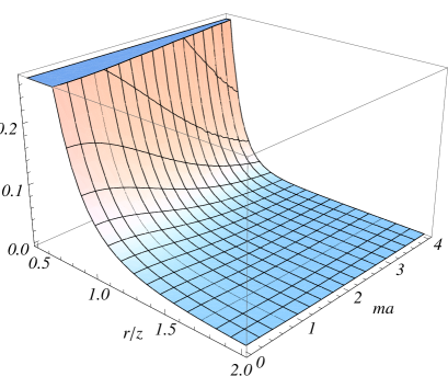
Figure 3: String-induced part in the VEV of the azimuthal stress, $a^{4}\langle T_{\phi}^{\phi}\rangle_{\mathrm{cs}}$, as a functions of the distance from the string and of the field mass in units of AdS curvature scale for the cosmic string with $q=3$.

The calculation of the axial stress, $\langle 0|T_{zz}|0\rangle$, becomes simpler because $\Gamma_{z}=0$. Substituting (31) and (32), and the corresponding gamma matrix into (59), after some intermediate steps we arrive at:

$$\langle 0|T_{zz}|0\rangle = -\frac{qz^{3}}{8\pi a^{2}}\sum_{\sigma}\frac{\lambda^{2}k^{2}}{E}\left[b_{s}^{(+)}J_{\beta_{1}}^{2}(\lambda r)-b_{s}^{(-)}J_{\beta_{2}}^{2}(\lambda r)\right]$$ (89)

$$\times\left[J_{\nu_{1}}(kz)J_{\nu_{2}}^{\prime}(kz)-J_{\nu_{2}}(kz)J_{\nu_{1}}^{\prime}(kz)\right]\ .$$

By using the recurrence relations involving the derivative of the Bessel function, taking the summations over $s$, and using (39) we get:

$$\langle 0|T_{zz}|0\rangle = \frac{qz^{3}}{\pi^{3/2}a^{2}}\int_{0}^{\infty}ds\int_{0}^{\infty}d\lambda\lambda e^{-\lambda^{2}s^{2}}\sum_{j}\left[J_{qj-1/2}^{2}(\lambda r)+J_{qj+1/2}^{2}(\lambda r)\right]$$ (90)

$$\int_{0}^{\infty}dkk^{3}e^{-k^{2}s^{2}}\left[J_{\nu_{1}}^{2}(kz)+J_{\nu_{2}}^{2}(kz)-\frac{2ma}{kz}J_{\nu_{1}}(kz)J_{\nu_{2}}(kz)\right]\ .$$

The procedure to evaluate the integrals is similar to the one we have adopted in the calculation of the radial stress. Introducing in the final result the new variable $y=r^{2}/(2s^{2})$, we obtain

$$\langle 0|T_{z}^{z}|0\rangle = \frac{q\rho^{-5}}{(2\pi)^{3/2}a^{4}}\int_{0}^{\infty}dy\ y^{3/2}e^{-(1+\rho^{-2})y}\mathcal{I}(q,y)$$ (91)

$$\times\left[I_{\nu_{1}}(y/\rho^{2})+I_{\nu_{2}}(y/\rho^{2})\right]\ .$$

By using (46) and extracting the part due to the pure AdS spacetime, we obtain the contribution to the axial stress induced by the cosmic string. The latter coincides with the corresponding expression for the energy density:

$$\langle T_{z}^{z}\rangle_{\mathrm{cs}}=\langle T_{0}^{0}\rangle_{\mathrm{cs}}\ .$$ (92)

By using the recurrence relations involving the derivative of the associated Legendre function, it can be explicitly checked that the part in the VEV of the energy-momentum tensor induced by the cosmic string obeys the covariant conservation equation, $\langle T_{\mu}^{\nu}\rangle_{\mathrm{cs};\nu}=0$, which for the problem under consideration is reduced to two differential equations,

$$\partial_{r}(r\langle T_{r}^{r}\rangle_{\mathrm{cs}})-\langle T_{\phi}^{\phi}\rangle_{\mathrm{cs}}=0\ ,$$

$$z\partial_{z}\langle T_{z}^{z}\rangle_{\mathrm{cs}}+\langle T_{\mu}^{\mu}\rangle_{\mathrm{cs}}-4\langle T_{z}^{z}\rangle_{\mathrm{cs}}=0\ .$$ (93)

Also, by using the recurrence relations involving the associated Legendre functions of different orders, it can be verified that the trace relation below is satisfied:

$$\langle T_{\mu}^{\mu}\rangle_{\mathrm{cs}}=m\langle\bar{\psi}\psi\rangle_{\mathrm{cs}}\ .$$ (94)

Note that the trace anomaly is contained in the pure AdS part of the VEV and the string-induced part is traceless for a massless fermionic field.

It is of interest to compare the results given above for the VEV of the energy-momentum tensor with the corresponding results for a scalar field discussed in [36]. In the case of the scalar field, the vacuum energy–momentum tensor, in general, is non-diagonal with the off-diagonal component $\langle T_{z}^{r}\rangle_{\mathrm{cs}}$. The latter vanishes for a conformally coupled massless field only. In this special case, the VEV of the energy-momentum tensor is conformally related to the corresponding quantity for the geometry of a cosmic string in flat spacetime with an additional flat boundary with Dirichlet boundary condition on it. Another difference in the VEVs for scalar and fermionic fields is that, in the scalar case the radial and axial stresses, in general, do not coincide with the energy density (no summation over $l$): $\langle T_{l}^{l}\rangle_{\mathrm{cs}}\neq\langle T_{0}^{0}\rangle_{\mathrm{cs}}$, $l=r,z$. At large distances from the string, for a scalar field the diagonal components of the VEV decay as $\langle T_{\mu}^{\mu}\rangle_{\mathrm{cs}}\propto(z/r)^{2\nu+3}$, where $\nu=\sqrt{9/4-12\xi+m^{2}a^{2}}$ and $\xi$ is the curvature coupling parameter. In particular, for a massive conformally coupled scalar field ($\xi=1/6$) the suppression of the VEVs is weaker than in the fermionic case with the same mass.

5 Conclusion

In this paper we have evaluated the FC and the VEV of the energy-momentum tensor associated with fermionic field on background of a four-dimensional AdS spacetime in the presence of a cosmic string. These VEVs are generated by the two sources of the vacuum polarization: by the gravitational field due to the negative cosmological constant and by non-trivial topology induced by the cosmic string. Because the analysis of quantum fermionic fields in a pure AdS space have been developed in the literature, here we are mainly interested in the calculation of the vacuum expectations values induced by the cosmic string. Moreover, because the presence of the string does not modify the curvature of the AdS background, all the divergences presented in the calculations of the VEVs, appear only in the contributions due the purely AdS space. So the contributions induced by the string do not require renormalization. All of them are automatically finite for points outside the string.

The evaluation of the above mentioned VEVs have been made by using the summation over the fermionic modes. So a crucial point in this paper was to obtain the complete set of fermionic wave-functions given by (27) and (31). In order to specify uniquely the mode-functions in AdS bulk, an additional boundary condition is required on the AdS boundary. Here, we consider a special case of boundary conditions, when the MIT bag boundary condition is imposed at a finite distance from the boundary, which is then taken to zero. By applying to the sum over the angular momentum the summation formula (46), the VEVs are decomposed as the sums of the pure AdS background and string-induced parts. In this way, for points away from the string, the renormalization is reduced to the one for the pure AdS bulk in the absence of the string. String-induced parts in both the FC and the VEV of the energy-momentum tensor depend on the coordinates $r$ and $z$ in the form of the combination $r/z$. The latter is the proper distance from the string measured in the units of AdS curvature radius. As partial check of the formulas for AdS bulk, we have shown that for large values of the curvature radius, to leading order, the VEVs are obtained for the geometry of cosmic string in Minkowski spacetime.

The string-induced part in the FC is given by the expression (48). At large proper distances from the string, the leading term in the corresponding asymptotic expansion is given by (51). For a fixed value of the radial coordinate $r$, the string-induced part in the FC vanishes on the AdS boundary. For a fixed value of $z$ and at large distances from the cosmic string, the string-induced part decays as $r^{-2ma-4}$. For a cosmic string in background of Minkowski spacetime and for a massive fermionic field, at large distances from the string the FC decays exponentially. At small proper distances from the string, the leading term in FC behaves as $(z/r)^{2}$. In particular, the FC diverges on the AdS horizon.

The VEV of the energy-momentum tensor is decomposed as (60). Because the maximal symmetry of the AdS bulk, the pure AdS part does not depend on the spacetime point and is proportional to the metric tensor. The string-induced part in the VEV of the energy-momentum tensor is diagonal and the corresponding axial and radial stresses are equal to the energy density. Note that, in the case of the scalar field, the vacuum energy–momentum tensor, in general, is non-diagonal with the off-diagonal component $\langle T_{z}^{r}\rangle_{\mathrm{cs}}$. Another difference in the VEVs for scalar and fermionic fields is that, in the scalar case the radial and axial stresses, in general, do not coincide with the energy density. For the fermionic field, the string-induced parts in the energy density and the azimuthal stress are given by the expressions (65) and (83). At large proper distances from the string, these parts are related to the FC by formulas (69) and (85) and the total VEV is dominated by the pure AdS part. At small proper distances from the string, the string-induced part behaves as $(z/r)^{4}$ and between the energy density and the azimuthal stress one has the relation (86). We have explicitly checked that the components of the string-induced part of the energy-momentum tensor obey the covariant conservation conditions, (93), and the trace relation, Eq. (94). The trace anomaly is contained in the pure AdS VEV and the string-induced part is traceless for a massless fermionic field.

In the geometry under consideration the boundary of AdS spacetime can be identified with a 3-dimensional conical spacetime. As it has been shown in [46], this spacetime arises as a solution of 3-dimensional Einstein equations in the presence of a point mass $m_{0}$. This mass is connected to the planar angle deficit by the relation $m_{0}=(1-1/q)/(4G_{3})$, where $G_{D}$ is the gravitational constant in $D$-dimensional spacetime. Note that the linear mass density of the string in 4-dimensional spacetime is given by $\mu_{0}=(1-1/q)/(4G_{4})$. Similar to AdS/CFT correspondence, a duality between the scalar field theories living in AdS bulk with an infinite static string and on its boundary has been discussed in [40]. Analogous duality between the fermionic field theories can be considered by using the standard prescription for fermion fields in AdS/CFT correspondence [47, 48] (for a recent discussion see also [49]). In this prescription the non-normalizable modes in AdS bulk are treated as source terms coupled to a fermionic operator $\mathcal{O}$ in the boundary theory which is dual to the fermionic field $\psi$. The quantization procedure we have used corresponds to, so called, standard quantization of fermionic fields in AdS/CFT correspondence. For $ma<1/2$ there is an alternative quantization procedure in which the boundary condition fixes the lower component of the bispinor. In this case one has two different dual theories on the boundary which are related by a Legendre transform. Having the expectation values for the bilinear products of the fermionic operators in the bulk one can investigate the corresponding expectation values in the dual theory by using the standard prescription for computing the two-point functions on the boundary. However, such a discussion is beyond the scope of the present paper.

Appendix A On the boundary condition at AdS boundary

Consider the fermionic field in the region $z>\delta$ assuming that on the boundary the field obeys the MIT bag boundary condition

$$(1+i\gamma^{\mu}n_{\mu})\psi=0,\;z=\delta,$$ (95)

with $n_{\mu}=-\delta_{\mu}^{z}a/z$ being the normal to the boundary. This boundary condition guarantees the zero flux of fermions through the boundary. The positive-energy mode functions for this problem are obtained from (27) with the replacements $C_{\sigma}^{(+)}\rightarrow C_{b\sigma}^{(+)}$ and $J_{\nu_{l}}(kz)\rightarrow J_{\nu_{l}}(kz)+CY_{\nu_{l}}(kz)$, $l=1,2$. From the boundary condition (95) it follows that $C=-J_{\nu_{2}}(k\delta)/Y_{\nu_{2}}(k\delta)$. The new normalization coefficient $C_{b\sigma}^{(+)}$ is determined from the normalization condition (29), where now the integration goes over the region $z\geqslant\delta$. By the calculations similar to those we have described in section 2, the following expression is obtained

$$|C_{b\sigma}^{(+)}|^{2}=\frac{sq\lambda^{2}k}{8\pi a^{3}Eb_{s}^{(+)}}\frac{Y_{\nu_{2}}^{2}(k\delta)}{J_{\nu_{2}}^{2}(k\delta)+Y_{\nu_{2}}^{2}(k\delta)}.$$ (96)

In this way, for the positive-energy fermionic mode functions, obeying the boundary condition (95), one gets

$$\psi_{b\sigma}^{(+)}(x)=C_{b\sigma}^{(+)}e^{-iEt}z^{2}\left(\begin{array}[]{c}J_{\beta_{1}}(\lambda r)V_{\nu_{1}}(kz)\\ -\epsilon_{j}b_{s}^{(+)}J_{\beta_{2}}(\lambda r)V_{\nu_{2}}(kz)e^{iq\phi}\\ isJ_{\beta_{1}}(\lambda r)V_{\nu_{2}}(kz)\\ i\epsilon_{j}sb_{s}^{(+)}J_{\beta_{2}}(\lambda r)V_{\nu_{1}}(kz)e^{iq\phi}\end{array}\right)e^{iq(j-1/2)\phi}\ ,$$ (97)

with the notation

$$V_{\nu}(kz)=J_{\nu}(kz)-\frac{J_{\nu_{2}}(k\delta)}{Y_{\nu_{2}}(k\delta)}Y_{\nu}(kz).$$ (98)

The expression for the negative-energy modes $\psi_{b\sigma}^{(-)}(x)$ is derived in a similar way. This expression is obtained from (31) by the replacements $C_{\sigma}^{(-)}\rightarrow C_{b\sigma}^{(-)}$ and $J_{\nu_{l}}(kz)\rightarrow V_{\nu_{l}}(kz)$, where $|C_{b\sigma}^{(-)}|^{2}$ is given by (96) with the change $b_{s}^{(+)}\rightarrow b_{s}^{(-)}$. In the limit $\delta\rightarrow 0$, for a fixed $z>\delta$, one has $|C_{b\sigma}^{(+)}|^{2}\rightarrow|C_{\sigma}^{(+)}|^{2}$, $V_{\nu_{l}}(kz)\rightarrow J_{\nu_{l}}(kz)$ and the mode functions $\psi_{b\sigma}^{(\pm)}(x)$ are reduced to (27) and (31), as it has been stated in the text.

References

- [1] S. J. Avis, C. J. Isham, D. Storey, Phys. Rev. D 18, 3565 (1978).
- [2] R. Camporesi, Phys. Rev. D 43, 3958 (1991).
- [3] M.M. Caldarelli, Nucl. Phys. B 549, 499 (1999).
- [4] R. Camporesi and A. Higuchi, Phys. Rev. D 45, 3591 (1992).
- [5] A. Flachi, I.G. Moss and D. Toms, Phys. Rev. D 64, 105029 (2001).
- [6] A. Flachi, I.G. Moss and D. Toms, Phys. Lett. B, 153 (2001).
- [7] S.-H. Shao, P. Chen and J.-A. Gu, Phys. Rev. D 81, 084036 (2010).
- [8] E. Elizalde, S.D. Odintsov and A.A. Saharian, arXiv:1302.2801.
- [9] O. Aharony, S.S. Gubser, J. Maldacena, H. Ooguri and Y. Oz, Phys. Rep. 323, 183 (2000).
- [10] P. Brax and C. Van de Bruck, Classical Quantum Gravity 20, R201 (2003); R. Maartens and K. Koyama, Living Rev. Relativity 13, 5 (2010).
- [11] T.W. Kibble, J. Phys. A 9, 1387 (1976).
- [12] A. Vilenkin and E.P.S. Shellard, Cosmic Strings and Other Topological Defects (Cambridge University Press, Cambridge, England, 1994).
- [13] V. Berezinski, B. Hnatyk and A. Vilenkin, Phys. Rev. D 64, 043004 (2001).
- [14] T. Damour and A. Vilenkin, Phys. Rev. Lett. 85, 3761 (2000).
- [15] P. Bhattacharjee and G. Sigl, Phys. Rep. 327, 109 (2000).
- [16] S. Sarangi and S.-H. Henry Tye, Phys. Lett. B 536, 185 (2002).
- [17] E.J. Copeland, R.C. Myers and J. Polchinski, J. High Energy Phys. 06, 013 (2004).
- [18] G. Dvali and A. Vilenkin, J. Cosmol. Astropart. Phys. 03, 010 (2004).
- [19] B. Linet, Phys. Rev. D, 35, 536 (1987).
- [20] A.G. Smith, in Symposium on the Formation and Evolution of Cosmic String, edited by G.W. Gibbons, S.W. Hawking and T. Vachaspati (Cambridge University Press, Cambridge, England, 1989).
- [21] P.C. Davies and V. Sahni, Class. Quantum Grav. 5 1 (1987).
- [22] T. Souradeep and V. Sahni, Phys. Rev. D 46, 1616 (1992).
- [23] M.E.X. Guimarães and B. Linet, Class. Quantum Grav. 10, 1665 (1993).
- [24] E.R. Bezerra de Mello, V.B. Bezerra, A.A. Saharian and A.S. Tarloyan, Phys. Rev. D 74, 025017 (2006).
- [25] V.P. Frolov and E.M. Serebriany, Phys. Rev. D 15, 3779 (1987).
- [26] B. Linet, J. Math. Phys. 36, 3694 (1995).
- [27] E.S. Moreira Jnr., Nucl. Phys. B 451, 365 (1995).
- [28] V.B. Bezerra and N.R. Khusnutdinov, Class. Quantum Grav. 23, 3449 (2006).
- [29] E.R. Bezerra de Mello, V.B. Bezerra, A.A. Saharian, and A.S. Tarloyan, Phys. Rev. D 78, 105007 (2008).
- [30] J.S. Dowker, Phys. Rev. D 36, 3742 (1987).
- [31] B. Allen, J.G. Mc.Lauglin and A.C. Ottewill, Phys. Rev. D 45, 4486 (1992).
- [32] E.R. Bezerra de Mello, V.B. Bezerra, and A.A. Saharian, Phys. Lett. B 645, 245 (2007).
- [33] A.C. Ottewill and P. Taylor, Class. Quantum Grav. 28, 015007 (2011).
- [34] E.R. Bezerra de Mello and A.A. Saharian, JHEP 04 (2009) 046.
- [35] E.R. Bezerra de Mello and A.A. Saharian, JHEP 08 (2010) 038.
- [36] E.R. Bezerra de Mello and A.A. Saharian, J. Phys. A: Math. Theor. 45, 115402 (2012).
- [37] A. Vilenkin, Phys. Rev. D 23, 852 (1981).
- [38] J. R. Gott III, Astrophys. J. 288, 422 (1985); W. Hiscock, Phys. Rev. D 31, 3288 (1985); B. Linet, Gen. Relativ. Gravit. 17, 1109 (1985); D. Garfinkle, Phys. Rev. D 32, 1323 (1985).
- [39] M.H. Dehghani, A.M. Ghezelbash and R.B. Mann, Nucl. Phys. B 625, 389 (2002).
- [40] C.A. Ballon Bayona, C.N. Ferreira and V.J. Vasquez Otoya, Class. Quantum Grav. 28, 015011 (2011).
- [41] J.D. Bjorken and S.D. Drell, Relativistic Quantum Mechanics (McGraw-Hill, New York, 1964).
- [42] I.S. Gradshteyn and I.M. Ryzhik. Table of Integrals, Series and Products (Academic Press, New York, 1980).
- [43] E.R. Bezerra de Mello, A.A. Saharian and S.V. Abajyan, Class. Quantum Grav. 30, 015002 (2013).
- [44] A. Erdélyi et al, Higher Transcendental Functions, Vol. 1 (McGraw Hill, New York, 1953).
- [45] Handbook of Mathematical Functions, edited by M. Abramowitz and I.A. Stegun (Dover, New York, 1972).
- [46] S. Deser, R. Jackiw, and G. ’t Hooft, Ann. Phys. 152, 220 (1984).
- [47] M. Henningson and K. Sfetsos, Phys. Lett. B 431, 63 (1998).
- [48] W. Mück and K.S. Viswanathan, Phys. Rev. D 58, 106006 (1998).
- [49] N. Iqbal and H. Liu, Fortsch.Phys. 57, 367 (2009).