Mansuripur’s paradox

Abstract

A recent article claims that the Lorentz force law is incompatible with special relativity. We discuss the “paradox” on which this claim is based. The resolution depends on whether one assumes a “Gilbert” model for the magnetic dipole (separated monopoles) or the standard “Ampère” model (a current loop). The former case was treated in these pages many years ago; the latter, as several authors have noted, constitutes an interesting manifestation of “hidden momentum.”

I Introduction

On May 7, 2012, a remarkable article appeared in Physical Review Letters. Man The author, Masud Mansuripur, claimed to offer “incontrovertible theoretical evidence of the incompatibility of the Lorentz [force] law with the fundamental tenets of special relativity,” and concluded that “the Lorentz law must be abandoned.” The Lorentz law,

$${\bf F}=q[{\bf E}+({\bf v}\times{\bf B})]$$ (1)

tells us the force F on a charge $q$ moving with velocity v through electric and magnetic fields E and B. Together with Maxwell’s equations, it is the foundation on which all of classical electrodynamics rests. If it is incorrect, 150 years of theoretical physics is in serious jeopardy.

Such a provocative proposal was bound to attract attention. Science SCI published a full-page commentary, and within days several rebuttals were posted. Reb Critics pointed out that since the Lorentz force law can be embedded in a manifestly covariant formulation of electrodynamics, it is guaranteed to be consistent with special relativity,COV and and some of them identified the specific source of Mansuripur’s error: neglect of “hidden momentum.” Nearly a year later Physical Review Letters published four rebuttals, YL and Science printed a follow-up article declaring the “purported relativity paradox resolved.” SCI2

Mansuripur’s argument is based on a “paradox” that was explored in this journal by Victor Namias and others Namias many years ago: a magnetic dipole moving through an electric field can experience a torque, with no accompanying rotation. In Section II we introduce Mansuripur’s version of the paradox, in simplified form, and explain Namias’s resolution. The latter is based on a “Gilbert” model of the dipole (separated magnetic monopoles); it does not work for the (realistic) “Ampère” model (a current loop). For Amperian dipoles the resolution involves “hidden” momentum, so in Section III we discuss the physical nature of this often-misunderstood phenomenon. Mansuripur himself treated the dipole as the point limit of a magnetized object, so in Section IV we repeat the calculations in that context (for both models), and confirm our earlier results. In Section V we discuss the Einstein–Laub force law, which Mansuripur proposed as a replacement for the Lorentz law, and in Section VI we offer some comments and conclusions.

II Gilbert Dipoles: Namias’s Resolution

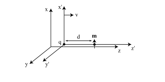
Figure 1: Electric charge ($q$) and magnetic dipole (m) in proper (primed) and lab (unprimed) frames.

First the paradox: In ${\cal S}^{\prime}$ (the “proper” frame) there is an ideal magnetic dipole ${\bf m}=m_{0}\,{\bf\hat{x}}$ at $(0,0,d)$, and a point charge $q$ at the origin, both at rest. The torque on m is (obviously) zero. Now examine the same configuration in ${\cal S}$ (the “lab” frame), with respect to which ${\cal S}^{\prime}$ moves at constant speed $v$ in the $z$ direction (Fig. 1). In ${\cal S}$ the (moving) point charge generates electric and magnetic fields

$${\bf E}(x,y,z,t) = \frac{q}{4\pi\epsilon_{0}}\frac{\gamma}{R^{3}}\left(x\,{\bf\hat{x}}+y\,{\bf\hat{y}}+(z-vt)\,{\bf\hat{z}}\right),$$ (2)

$${\bf B}(x,y,z,t) = \frac{q}{4\pi\epsilon_{0}}\frac{v\gamma}{c^{2}R^{3}}\left(-y\,{\bf\hat{x}}+x\,{\bf\hat{y}}\right),$$ (3)

($\gamma\equiv 1/\sqrt{1-(v/c)^{2}}$, $R\equiv\sqrt{x^{2}+y^{2}+\gamma^{2}(z-vt)^{2}}\,$), and the (moving) magnetic dipole acquires an electric dipole moment VH

$${\bf p}=\frac{1}{c^{2}}({\bf v}\times{\bf m})=\frac{1}{c^{2}}vm_{0}\,{\bf\hat{y}}.$$ (4)

The torque on the dipole is

$${\bf N}=({\bf m}\times{\bf B})+({\bf p}\times{\bf E})=\frac{qm_{0}}{4\pi\epsilon_{0}}\frac{v}{c^{2}d^{2}}\,{\bf\hat{x}}$$ (5)

(by Lorentz transformation, $d=\gamma(z-vt)$; the magnetic contribution is zero, because B vanishes on the $z$ axis). The torque is zero in one inertial frame, but non-zero in the other! Mansuripur concludes that the Lorentz force law (on which Eq. 5 is predicated) is inconsistent with special relativity.

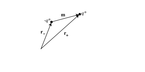
Figure 2: “Gilbert” magnetic dipole.

This “paradox” was resolved years ago by Victor Namias. Namias The standard torque formulas (${\bf p}\times{\bf E}$ and ${\bf m}\times{\bf B}$) apply to dipoles at rest, but they do not hold, in general, for dipoles in motion. Suppose we model the magnetic dipole as separated monopoles (Fig. 2). The “Lorentz force law” for a magnetic monopole $q^{*}$ reads DJG1

$${\bf F}=q^{*}\left[{\bf B}-(1/c^{2}){\bf v}\times{\bf E}\right],$$ (6)

so the torque origin on a moving dipole ${\bf m}=q^{*}({\bf r}_{+}-{\bf r}_{-})$ is

$${\bf N} = ({\bf r}_{+}\times{\bf F}_{+})+({\bf r}_{-}\times{\bf F}_{-})$$

$$= ({\bf m}\times{\bf B})-\frac{1}{c^{2}}{\bf m}\times({\bf v}\times{\bf E}).$$

But ${\bf m}\times({\bf v}\times{\bf E})={\bf v}\times({\bf m}\times{\bf E})+({\bf m}\times{\bf v})\times{\bf E}$, so

$${\bf N} = ({\bf m}\times{\bf B})-\frac{1}{c^{2}}({\bf m}\times{\bf v})\times{\bf E}-\frac{1}{c^{2}}{\bf v}\times({\bf m}\times{\bf E})$$ (7)

$$= ({\bf m}\times{\bf B})+({\bf p}\times{\bf E})-\frac{1}{c^{2}}{\bf v}\times({\bf m}\times{\bf E}).$$

There is a third term, missing in Eq. 5, which (it is easy to check) exactly cancels the offending torque; the net torque is zero in both frames.

III Ampère Dipoles: Hidden Momentum

Namias believed that his formula (Eq. 7) applies just as well to an Ampère dipole as it does to a Gilbert dipole. He was mistaken. An Ampère dipole in an electric field carries “hidden” momentum, hid_mom

$${\bf p}_{h}=\frac{1}{c^{2}}({\bf m}\times{\bf E}).$$ (8)

Because it is crucial in understanding the resolution to Mansuripur’s paradox, we pause to review the derivation of this formula, in a simple model.

Imagine a rectangular loop of wire carrying a steady current. Picture the current as a stream of noninteracting positive charges that move freely within the wire. UN When a uniform electric field E is applied (Fig. 3), the charges accelerate up the left segment, and decelerate down the right one. Question: What is the total momentum of all the charges in the loop? The left and right segments cancel, so we need only consider the top and bottom. Say there are $N_{t}$ charges in the top segment, going to the right at speed $v_{t}$, and $N_{b}$ charges in the lower segment, going at (slower) speed $v_{b}$ to the left. The current ($I=\lambda v$) is the same in all four segments (otherwise charge would be piling up somewhere). Thus

$$I={qN_{t}\over l}v_{t}={qN_{b}\over l}v_{b},\quad{\rm so}\quad N_{t}v_{t}=N_{b}v_{b}={Il\over q},$$ (9)

where $q$ is the charge of each particle, and $l$ is the length of the rectangle. Classically, the momentum of a single particle is $p=mv$, where $m$ is its mass, so the total momentum (to the right) is

$$p_{\rm classical}=mN_{t}v_{t}-mN_{b}v_{b}=m{Il\over q}-m{Il\over q}=0,$$ (10)

as one would certainly expect (after all, the loop as a whole is not moving). But relativistically the momentum of a particle is $p=\gamma mv$, and we get

$$p_{\rm relativistic}=\gamma_{t}mN_{t}v_{t}-\gamma_{b}mN_{b}v_{b}={mIl\over q}\left(\gamma_{t}-\gamma_{b}\right),$$ (11)

which is not zero, because the particles in the upper segment are moving faster. In fact, the gain in energy ($\gamma mc^{2}$), as a particle goes up the left side, is equal to the work done by the electric force, $qEw$, where $w$ is the height of the rectangle, so

$$\gamma_{t}-\gamma_{b}={qEw\over mc^{2}},\quad{\rm and\ hence}\quad p_{\rm rel}={IlEw\over c^{2}}.$$ (12)

Now $Ilw$ is the magnetic dipole moment of the loop; as vectors, m points into the page and p is to the right, so

$${\bf p}_{\rm rel}={1\over c^{2}}({\bf m}\times{\bf E}).$$ (13)

This is the “hidden” momentum in Eq. 8.

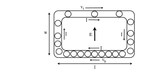
Figure 3: Current loop in an external electric field.

The term “hidden momentum” was coined by Shockley; hid_mom it was an unfortunate choice. The phenomenon itself was first studied in the context of static electromagnetic systems with nonzero field momentum (${\bf p}_{\rm field}=\epsilon_{0}\int({\bf E}\times{\bf B})\,d^{3}{\bf r}$). In such configurations the hidden momentum exactly cancels the field momentum (${\bf p}_{h}=-{\bf p}_{\rm field}$), leaving a total of zero, as required by the “center of energy theorem.” CET This has created the impression that hidden momentum is something artificial and ad hoc—invented simply to rescue an abstract theorem. ABS   Nothing could be farther from the truth. Hidden momentum is perfectly ordinary relativistic mechanical momentum, as the example above indicates; it occurs in systems with internally moving parts, such as current-carrying loops, and it is “hidden” only in the sense that it not associated with motion of the object as a whole. A Gilbert dipole in an electric field, having no moving parts, harbors no hidden momentum (and the fields—with the crucial delta-function term in B included—carry no compensating momentum). HM

Returning to the configuration in Fig. 1, the hidden momentum in ${\cal S}^{\prime}$ is

$${\bf p}_{h}=\frac{1}{c^{2}}\left[(m_{0}\,{\bf\hat{x}})\times\left(\frac{1}{4\pi\epsilon_{0}}\frac{q}{d^{2}}\,{\bf\hat{z}}\right)\right]=-\frac{qm_{0}}{4\pi\epsilon_{0}c^{2}d^{2}}\,{\bf\hat{y}}.$$ (14)

Because ${\bf p}_{h}$ is perpendicular to v, and transverse components are unaffected by Lorentz transformations, this is also the hidden momentum in $\cal S$. It is constant (in time), so there is no associated force. But the hidden angular momentum,

$${\bf L}_{h}={\bf r}\times{\bf p}_{h},$$ (15)

is not constant (in the lab frame), because r is changing. In fact,

$$\frac{d{\bf L}_{h}}{dt}={\bf v}\times{\bf p}_{h}=\frac{qm_{0}}{4\pi\epsilon_{0}}\frac{v}{c^{2}d^{2}}\,{\bf\hat{x}}.$$ (16)

This increase in angular momentum requires a torque,

$${\bf N}=\frac{qm_{0}}{4\pi\epsilon_{0}}\frac{v}{c^{2}d^{2}}\,{\bf\hat{x}},$$ (17)

and this is precisely what we found in Eq. 5.

Recapitulating: In the Gilbert model there is an extra term in the torque formula (Eq. 7); the total torque is zero, there is no hidden angular momentum, and nothing rotates. In the Ampère model there is no third term in the torque formula (Eq. 5)NTT ; the torque is not zero, and drives the increasing hidden angular momentum—but still nothing rotates.lab_torque It helps to separate the angular momentum into two types: “overt” (associated with actual rotation) and “hidden” (so called because it is not associated with any overt rotation of the object). Torque is the rate of change of the total angular momentum:

$${\bf N}=\frac{d{\bf L}_{o}}{dt}+\frac{d{\bf L}_{h}}{dt}.$$ (18)

In both models $d{\bf L}_{o}/dt={\bf 0}$. In the Gilbert model N and $d{\bf L}_{h}/dt$ are also zero; in the Ampère model they are equal but non-zero.

IV Magnetized Materials

It is of interest to see how this plays out in Mansuripur’s formulation of the problem. He treats the dipole as magnetized medium, and calculates the torque directly from the Lorentz force law, without invoking ${\bf p}\times{\bf E}$ or ${\bf m}\times{\bf B}$. In the proper frame, he takes

$${\bf M}^{\prime}(x^{\prime},y^{\prime},z^{\prime},t^{\prime})=m_{0}\delta(x^{\prime})\delta(y^{\prime})\delta(z^{\prime}-d)\,{\bf\hat{x}}.$$ (19)

Now, M and P constitute an antisymmetric second-rank tensor:

$$P^{\mu\nu}=\begin{pmatrix}0&cP_{x}&cP_{y}&cP_{z}\\ -cP_{x}&0&-M_{z}&M_{y}\\ -cP_{y}&M_{z}&0&-M_{x}\\ -cP_{z}&-M_{y}&M_{x}&0,\end{pmatrix}$$ (20)

and the transformation rule is DJG2

$$P_{z}=P_{z}^{\prime},\ P_{x}=\gamma(P_{x}^{\prime}+\frac{v}{c^{2}}M_{y}^{\prime}),\ P_{y}=\gamma(P_{y}^{\prime}-\frac{v}{c^{2}}M_{x}^{\prime})$$

$$M_{z}=M_{z}^{\prime},\ M_{x}=\gamma(M_{x}^{\prime}-vP_{y}^{\prime}),\ M_{y}=\gamma(M_{y}^{\prime}+vP_{x}^{\prime})$$

(for motion in the $z$ direction). In the present case, then, the polarization and magnetization in the “lab” frame are

$${\bf M}(x,y,z,t) = m_{0}\delta(x)\delta(y)\delta\left(z-vt-(d/\gamma)\right){\bf\hat{x}},$$ (21)

$${\bf P}(x,y,z,t) = \frac{m_{0}v}{c^{2}}\delta(x)\delta(y)\delta\left(z-vt-(d/\gamma)\right){\bf\hat{y}}.$$ (22)

According to the Lorentz law, the force density is

$${\bf f}=\rho{\bf E}+{\bf J}\times{\bf B},$$ (23)

where $\rho=-\mbox{\boldmath$\nabla$}\mbox{\boldmath$\,\cdot\,$}{\bf P}$ is the bound charge density and ${\bf J}=\partial{\bf P}/\partial t+\mbox{\boldmath$\nabla$}\times{\bf M}$ is the sum of the polarization current and the bound current density. Using Eqs. 2, 3, 21, and 22, we obtain

$${\bf f} = -(\mbox{\boldmath$\nabla$}\mbox{\boldmath$\,\cdot\,$}{\bf P}){\bf E}+(\mbox{\boldmath$\nabla$}\times{\bf M})\times{\bf B}+\frac{\partial{\bf P}}{\partial t}\times{\bf B}$$ (24)

$$= -\frac{qm_{0}v}{4\pi\epsilon_{0}c^{2}}\frac{d}{R^{3}}\delta(x)\delta^{\prime}(y)\delta(z-vt-d/\gamma)\,{\bf\hat{z}}$$

(where a prime denotes the derivative). The net force on the dipole is

$${\bf F}=\int{\bf f}\,dx\,dy\,dz=\frac{qm_{0}vd}{4\pi\epsilon_{0}c^{2}}\frac{d}{dy}\left[\frac{1}{(y^{2}+d^{2})^{3/2}}\right]\Bigg{|}_{y=0}\,{\bf\hat{z}}={\bf 0}.$$ (25)

Meanwhile, the torque density is

$${\bf n}={\bf r}\times{\bf f}=-\frac{qm_{0}vd}{4\pi\epsilon_{0}c^{2}}\frac{y}{R^{2}}\delta(x)\delta^{\prime}(y)\delta(z-vt-d/\gamma)\,{\bf\hat{x}},$$ (26)

so the net torque on the dipole is

$${\bf N} = \int{\bf n}\,dx\,dy\,dz$$ (27)

$$= -\frac{qm_{0}vd}{4\pi\epsilon_{0}c^{2}}\left\{-\frac{d}{dy}\left[\frac{y}{(y^{2}+d^{2})^{3/2}}\right]\right\}\Bigg{|}_{y=0}\,{\bf\hat{x}}$$

$$= \frac{qm_{0}v}{4\pi\epsilon_{0}c^{2}d^{2}}\,{\bf\hat{x}},$$

confirming Eq. 5. This is the torque required to account for the increase in hidden angular momentum.

What if we run Mansuripur’s calculation for a dipole made out of magnetic monopoles? The bound charge, bound current, and magnetization current are minus

$$\rho^{*}_{b}=-\mbox{\boldmath$\nabla$}\mbox{\boldmath$\,\cdot\,$}{\bf M},\quad{\bf J}^{*}_{b}=-c^{2}\mbox{\boldmath$\nabla$}\times{\bf P},\quad{\bf J}^{*}_{p}=\frac{\partial{\bf M}}{\partial t},$$ (28)

so the force density on the magnetic dipole (again invoking Eqs. 2, 3, 21, and 22) isLFL

$${\bf f} = \rho^{*}{\bf B}-\frac{1}{c^{2}}{\bf J}^{*}\times{\bf E}$$ (29)

$$= -(\mbox{\boldmath$\nabla$}\mbox{\boldmath$\,\cdot\,$}{\bf M}){\bf B}+(\mbox{\boldmath$\nabla$}\times{\bf P})\times{\bf E}-\frac{1}{c^{2}}\left(\frac{\partial{\bf M}}{\partial t}\right)\times{\bf E}$$

$$= {\bf 0}.$$

The total force is again zero, but this time so too is the torque density (${\bf n}={\bf r}\times{\bf f}$), and hence the total torque. As before, the torque is zero in the Gilbert model—and there is no hidden angular momentum.

V The Einstein–Laub Force Law

Having concluded that the Lorentz force law is unacceptable, Mansuripur proposes to replace Eq. 24 with an expression based on the Einstein–Laub law: EL

$${\bf f}_{\rm EL} = ({\bf P}\mbox{\boldmath$\,\cdot\,$}\mbox{\boldmath$\nabla$}){\bf E}+\frac{\partial\bf P}{\partial t}\times(\mu_{0}{\bf H})+({\bf M}\mbox{\boldmath$\,\cdot\,$}\mbox{\boldmath$\nabla$})\mu_{0}{\bf H}$$ (30)

$$-\ \frac{1}{c^{2}}\,\frac{\partial\bf M}{\partial t}\times{\bf E}$$

$$= \frac{m_{0}qv\gamma}{4\pi\epsilon_{0}c^{2}}\frac{1}{R^{3}}\delta(x)\delta(y)[2\delta(z-vt-d/\gamma)$$

$$-\,(z-vt)\delta^{\prime}(z-vt-d/\gamma)]\,{\bf\hat{y}}.$$

The total force on the dipole still vanishes:

$${\bf F}_{\rm EL} = \frac{m_{0}qv\gamma}{4\pi\epsilon_{0}c^{2}}\,{\bf\hat{y}}\left\{\frac{2}{d^{3}}+\frac{1}{\gamma^{3}}\frac{d}{dz}\left[\frac{1}{(z-vt)^{2}}\right]\Bigg{|}_{z-vt=d/\gamma}\right\}$$ (31)

$$= {\bf 0}.$$

The torque density should be ${\bf r}\times{\bf f}_{\rm EL}$:

$${\bf n}_{\rm EL} = -\frac{m_{0}qv\gamma}{4\pi\epsilon_{0}c^{2}}\frac{z}{R^{3}}\delta(x)\delta(y)[2\delta(z-vt-d/\gamma)$$ (32)

$$\quad-\,(z-vt)\delta^{\prime}(z-vt-d/\gamma)]\,{\bf\hat{x}},$$

giving a total torque

$${\bf N}_{\rm EL} = -\,\frac{m_{0}qv\gamma}{4\pi\epsilon_{0}c^{2}}\,{\bf\hat{x}}\left\{\frac{2(vt+d/\gamma)}{d^{3}}+\frac{1}{\gamma^{3}}\frac{d}{dz}\left[\frac{z}{(z-vt)^{2}}\right]\right\}$$ (33)

$$= -\frac{m_{0}qv}{4\pi\epsilon_{0}c^{2}d^{2}}\,{\bf\hat{x}}$$

(the derivative is again evaluated at $z-vt=d/\gamma$). It’s not zero! In fact, it’s minus the “Lorentz” torque, Eq. 27. But Mansuripur argues that, “To guarantee the conservation of angular momentum, [Eq. 32] must be supplemented …”

$${\bf n}_{\rm EL}^{\prime}={\bf n}_{\rm EL}+({\bf P}\times{\bf E})+({\bf M}\times{\bf B}).$$ (34)

In our case the extra terms are

$$({\bf P}\times{\bf E})+({\bf M}\times{\bf B})=\frac{m_{0}qv}{4\pi\epsilon_{0}c^{2}d^{2}}\delta(x)\delta(y)\delta(z-vt-d/\gamma)\,{\bf\hat{x}},$$

and their contribution to the total torque is

$$\int[({\bf P}\times{\bf E})+({\bf M}\times{\bf B})]\,dx\,dy\,dz=\frac{m_{0}qv}{4\pi\epsilon_{0}c^{2}d^{2}}\,{\bf\hat{x}},$$ (35)

which is just right to cancel Eq. 33, yielding a net torque of zero (which Mansuripur takes to be the correct answer).

What are we to make of this argument? In the first place, the Einstein–Laub force density was derived assuming that the medium is at rest,EL which in this case it is not. More important, the magnetization terms implicitly assume a Gilbert model for the magnetic dipole:

$$({\bf M}\mbox{\boldmath$\,\cdot\,$}\mbox{\boldmath$\nabla$}){\bf B}=-\mbox{\boldmath$\nabla$}\times({\bf M}\times{\bf B})+({\bf B}\mbox{\boldmath$\,\cdot\,$}\mbox{\boldmath$\nabla$}){\bf M}-(\mbox{\boldmath$\nabla$}\mbox{\boldmath$\,\cdot\,$}{\bf M}){\bf B};$$ (36)

as long as the magnetization is localized, the first two terms yield vanishing surface integrals, SUI leaving $-(\mbox{\boldmath$\nabla$}\mbox{\boldmath$\,\cdot\,$}{\bf M}){\bf B}-(1/c^{2})[(\partial{\bf M}/\partial t)\times{\bf E}]$ for the net force density on the object, the same as in the Gilbert model (Eq. 29). Tellegen There may be some contexts in which the Einstein–Laub force law is valid and useful, but this is not one of them. Mansuripur is quite explicit in writing that the magnetic dipole he has in mind is “a small, charge neutral loop of current,” which is to say, an Ampère dipole.

VI Conclusion

The resolution of Mansuripur’s “paradox” depends on the model for the magnetic dipole:

• If it is a Gilbert dipole (made from magnetic monopoles), the third term in Namias’s formula (Eq. 7) supplies the missing torque. In Mansuripur’s formulation (using a polarizable medium), it comes from a correct accounting of the bound charge/current (Eq. 28). The net torque is zero in the lab frame, just as it is in the proper frame.

• If it is an Ampère dipole (an electric current loop), the third term in Namias’s equation is absent, and the torque on the dipole is not zero. It is, however, just right to account for the increasing hidden angular momentum in the dipole.

In either model the Lorentz force law is entirely consistent with special relativity.

We thank Kirk McDonald, Daniel Vanzella, and Daniel Cross for useful correspondence. VH coauthored this paper in his private capacity; no official support or endorsement by the Centers for Disease Control and Prevention is intended or should be inferred.

References

- (1) M. Mansuripur, “Trouble with the Lorentz Law of Force: Incompatibility with Special Relativity and Momentum Conservation,” Phys. Rev. Lett. 108, 193901(4) (2012).
- (2) A. Cho, “Textbook Electrodynamics May Contradict Relativity,” Science 336, 404 (2012).
- (3) K. T. McDonald, “Mansuripur’s Paradox,” www.physics.princeton.edu/mcdonald/examples/mansuripur.pdf (14 pp); D. A. T. Vanzella, “Comment on ‘Trouble with the Lorentz law of force,’” e-print arXiv:1205.1502 (2 pp); D. J. Cross, “Resolution of the Mansuripur Paradox,” e-print arXiv:1205:5451 (3 pp); P. L. Saldanha, “Comment on ‘Trouble with the Lorentz law of force,’” e-print arXiv:1205:6858 (2 pp); D. J. Griffiths and V. Hnizdo, “Comment on ‘Trouble with the Lorentz law of force,’” e-print arXiv:1205.4646 (3 pp). Later critiques include K. A. Milton and G. Meille, “Electromagnetic Angular Momentum and Relativity,” e-print arXiv:1208:4826 (4 pp); F. De Zela, “Comment on ‘Trouble with the Lorentz law of force,’” e-print arXiv:1210.7344 (2 pp); T. M. Boyer, “Examples and comments related to relativity controversies,” Am. J. Phys. 80, 962-971 (2012); A. L. Kholmetskii, O. V. Missevitch, and T. Yarman, “Torque on a Moving Electric/Magnetic Dipole,” Prog. Elecromagnetics Research B, 45, 83-99 (2012). See also M. Mansuripur, “Trouble with the Lorentz Law of Force: Response to Critics,” Proc. SPIE, 8455, 845512 (2012).
- (4) The details are worked out in Cross and Vanzella (ref. 3).
- (5) D. A. T. Vanzella,“Comment on ‘Trouble with the Lorentz Law of Force: Incompatibility with Special Relativity and Momentum Conservation,’” Phys. Rev. Lett. 110, 089401-1 (2013); and, under the same title, S. M. Barnett, Phys. Rev. Lett. 110, 089402-1 (2013); P. L. Saldanha, Phys. Rev. Lett. 110, 089403-1-2 (2013); M. Khorrami, Phys. Rev. Lett. 110, 089404-1 (2013).
- (6) “Paradox Lost,” Science 339, 496 (2013); A. Cho, “Purported Relativity Paradox Resolved,” http://scim.ag/Lorpara (2013). Mansuripur himself does not accept this verdict, though he does appear to have softened his assertions somewhat: M. Mansuripur, “Mansuripur replies,” Phys. Rev. Lett. 110, 089405-1 (2013).
- (7) V. Namias, “Electrodynamics of moving dipoles: The case of the missing torque,” Am. J. Phys. 57, 171-177 (1989); D. Bedford and P. Krumm, “On the origin of magnetic dynamics,” Am. J. Phys. 54, 1036-1039 (1986).
- (8) See, for instance, V. Hnizdo, “Magnetic dipole moment of a moving electric dipole,” Am. J. Phys. 80, 645-647 (2012).
- (9) See, for example, D. J. Griffiths, Introduction to Electrodynamics, 4th ed. (Pearson, Boston, 2013), Eq. 7.69.
- (10) We calculate all torques (in the lab frame) with respect to the origin. But because the net force on the dipole is zero in all cases, it does not matter—we could as well use any fixed point, including the (instantaneous) position of the dipole.
- (11) W. Shockley and R. P. James, “‘Try simplest cases’ discovery of ‘hidden momentum’ forces on ‘magnetic currents,’” Phys. Rev. Lett. 18, 876-879 (1967); W. H. Furry, “Examples of momentum distributions in the electromagnetic field and in matter,” Am. J. Phys. 37, 621-636 (1969); L. Vaidman, “Torque and force on a magnetic dipole,” Am. J. Phys. 58, 978-983 (1990); V. Hnizdo, “Conservation of linear and angular momentum and the interaction of a moving charge with a magnetic dipole,” Am. J. Phys. 60, 242-246 (1992); V. Hnizdo, “Hidden mechanical momentum and the field momentum in stationary electromagnetic and gravitational systems,” Am. J. Phys. 65, 515-518 (1997).
- (12) This is of course an unrealistic model for an actual current-carrying wire. Vaidman (Ref. 11) explores more plausible models, but the result is unchanged.
- (13) If the center of energy of a closed system is at rest, the total momentum of the system must be zero. See, for example, S. Coleman and J. H. Van Vleck, “Origin of ‘Hidden Momentum Forces’ on Magnets,” Phys. Rev. 171, 1370-1375 (1968); M. G. Calkin, “Linear momentum of the source of a static electromagnetic field,” Am. J. Phys. 39, 513-516 (1971).
- (14) Mansuripur variously calls hidden momentum an “absurdity” (M. Mansuripur, “Resolution of the Abraham-Minkowski controversy,” Opt. Commun. 283, 1997-2005 (2010), p. 1999), a “problem” to be “solved” (Ref. 1) and “as applied to magnetic materials …an unnecessary burden” (Ref. 6).
- (15) D. J. Griffiths, “Dipoles at rest,” Am. J. Phys. 60, 979-987 (1992). The magnetic field of a point dipole is where for Ampère dipoles and for Gilbert dipoles. The delta function term leads, for example, to hyperfine splitting in the ground state of hydrogen, and provides experimental confirmation that the proton is an Ampére dipole.
- (16) We do not know a simple way to prove this directly, but we will confirm it implicitly in Section IV.
- (17) This is certainly not the first time such issues have arisen. How can there be a torque in the lab frame, when there is none in the proper frame? See J. D. Jackson, “Torque or no torque? Simple charged particle motion observed in different inertial frames,” Am. J. Phys. 72, 1484-1487 (2004). How can there be a torque, with no accompanying rotation? See D. G. Jensen, “The paradox of the L-shaped object,” Am. J. Phys. 57, 553-555 (1989).
- (18) See, for instance, Ref. 9, Eq. 12.118.
- (19) The minus sign in is due to the switched sign in “Ampère’s law” for magnetic monopoles (see Ref. 9, Eq. 7.44). Note that in Eq. 28 (and hence also Eq. 29), M and P are the densities of the dipole moments of magnetic monopoles and magnetic-monopole currents, respectively.
- (20) There is some dispute as to the correct form of the Lorentz force law for magnetic monopoles in the presence of polarizable and magnetizable materials, but not when (as here) the polarization/magnetization is itself due to monopoles. See K. T. McDonald, “Poynting’s Theorem with Magnetic Monopoles,” (11 pp), http://puhep1.princeton.edu/mcdonald/examples/poynting.pdf (2013).
- (21) A. Einstein and J. Laub, “Über die im elektromagnetischen Felde auf ruhende Körper ausgeübten ponderomotorischen Kräfte,” Ann. Phys. (Leipzig) 26, 541–550 (1908); English translation in The Collected Papers of Albert Einstein, Vol. 2 (Princeton University Press, Princeton, NJ, 1989). In evaluating the force, Mansuripur uses the field due to (see Eq. 12b in Ref. 1); his is our B (Eq. 3).
- (22) The th component of the second term is .
- (23) B. D. H. Tellegen, “Magnetic-dipole models,” Am. J. Phys. 30, 650–652 (1962). Tellegen’s force (6), which assumes a Gilbert magnetic dipole, can be obtained by integrating the magnetization-dependent terms in the Einstein–Laub force density in which it is assumed that . Another derivation of the force on a Gilbert magnetic dipole is by A. D. Yaghjian, “Electromagnetic forces on point dipoles,” IEEE Anten. Prop. Soc. Symp. 4, 2868–2871 (1999).