A scaling law beyond Zipf’s law and its relation to Heaps’ law

Abstract

The dependence on text length of the statistical properties of word occurrences has long been considered a severe limitation on the usefulness of quantitative linguistics. We propose a simple scaling form for the distribution of absolute word frequencies that brings to light the robustness of this distribution as text grows. In this way, the shape of the distribution is always the same, and it is only a scale parameter that increases (linearly) with text length. By analyzing very long novels we show that this behavior holds both for raw, unlemmatized texts and for lemmatized texts. In the latter case, the distribution of frequencies is well approximated by a double power law, maintaining the Zipf’s exponent value $\gamma\simeq 2$ for large frequencies but yielding a smaller exponent in the low-frequency regime. The growth of the distribution with text length allows us to estimate the size of the vocabulary at each step and to propose a generic alternative to Heaps’ law, which turns out to be intimately connected to the distribution of frequencies, thanks to its scaling behavior.

I Introduction

Zipf’s law is perhaps one of the best pieces of evidence about the existence of universal physical-like laws in cognitive science and the social sciences. Classic examples where it applies include the population of cities, company income, and the frequency of words in texts or speech Zipf (1949). In the latter case, the law is obtained directly by counting the number of repetitions, i.e., the absolute frequency $n$, of all words in a long enough text, and assigning increasing ranks, $r=1,2,\dots$, to decreasing frequencies. When a power-law relation

$$n\propto\frac{1}{r^{\beta}}$$

holds for a large enough range, with the exponent $\beta$ more or less close to 1, Zipf’s law is considered to be fullfilled (with $\propto$ denoting proportionality). An equivalent formulation of the law is obtained in terms of the probability distribution of the frequency $n$, such that it plays the role of a random variable, for which a power-law distribution

$$D(n)\propto\frac{1}{n^{\gamma}},$$

should hold, with $\gamma=1+1/\beta$ (taking values close to 2) and $D(n)$ as the probability mass function of $n$ (or the probability density of $n$, in a continuous approximation) Mandelbrot (1961); Ferrer i Cancho and Hernández-Fernández (2008); Adamic and Huberman (2002); Kornai (2002); Zanette (2012). Note that this formulation implies performing double statistics (i.e., doing statistics twice), first counting words to get frequencies and then counting repetition of frequencies to get the distribution of frequencies.

The criteria for the validity of Zipf’s law are arguably rather vague (long enough text, large enough range, exponent $\beta$ more or less close to 1). Generally, a long enough text means a book, a large range can be a bit more than an order of magnitude, and the proximity of the exponent $\beta$ to 1 translates into an interval (0.7,1.2), or even beyond that Zanette and Montemurro (2005); Zanette (2012); Ferrer i Cancho (2005a). Moreover, no rigorous methods have been usually required for the fitting of the power-law distribution: Linear regression in double-logarithmic scale is the most common method, either for $n(r)$ or for $D(n)$, despite the fact that it is well known that this procedure suffers from severe drawbacks and can lead to flawed results Clauset et al. (2009); Corral et al. (2011). Nevertheless, once these limitations are assumed, the fulfillment of Zipf’s law in linguistics is astonishing, being valid no matter the author, style, or language Zipf (1949); Zanette and Montemurro (2005); Zanette (2012). So, the law is universal, at least in a qualitative sense.

At a theoretical level, many different competing explanations of Zipf’s law have been proposed Zanette (2012), such as random (monkey) typing Miller (1957); Li (1992) ,preferential repetitions or proportional growth Simon (1955); Newman (2005); Saichev et al. (2009), the principle of least effort Zipf (1949); Ferrer i Cancho and Solé (2003); Corominas-Murtra et al. (2011); Ferrer i Cancho (2005b), and, beyond linguistics, Boltzmann-type approaches Düring et al. (2009), or even avalanche dynamics in a critical system Bak (1996); most of these options have generated considerable controversy Mitzenmacher (2004); Ferrer i Cancho and Elvevåg (2010); Dickman et al. (2012). In any case, the power-law behavior is the hallmark of scale invariance, i.e., the impossibility to define a characteristic scale, either for frequencies or for ranks. Although power laws are sometimes also referred to as scaling laws, we will make a more precise distinction here. In short, a scaling law is any function invariant under a scale transformation (which is a linear dilation or contraction of the axes). In one dimension the only scaling law is the power law, but this is not true with more than one variable Christensen and Moloney (2005). Note that in text statistics, other variables to consider in addition to frequency are the text length $L$ (the total number of words, or tokens) and the size of the vocabulary $V_{L}$ (i.e., the number of different words, or types).

Somehow related to Zipf’s law is Heaps’ law (also called Herdan’s law Baayen (2001); Herdan (1964)), which states that the vocabulary $V_{L}$ grows as a function of the text length $L$ as a power law,

$$V_{L}\propto L^{\alpha},$$

with the exponent $\alpha$ smaller than one. However, even simple log-log plots of $V_{L}$ versus $L$ do not show a convincing linear behavior Gerlach and Altmann (2013) and therefore, the evidence for this law is somewhat weak (for a notable exception see Ref. Kornai (2002)). Nevertheless, a number of works have derived the relationship $\beta=1/\alpha$ between Zipf’s and Heaps’ exponents Mandelbrot (1961); Kornai (2002); van Leijenhorst and van der Weide (2005), at least in the infinite-system limit Serrano et al. (2009); Lü et al. (2010), using different assumptions.

Despite the relevance of Zipf’s law, and its possible relations with criticality, few systematic studies about the dependence of the law on system size (i.e., text length) have been carried out. It was Zipf himself (Zipf, 1949, pp. 144) who first observed a variation in the exponent $\beta$ when the system size was varied. In particular, “small” samples would give $\beta<1$, while “big” ones yielded $\beta>1$. However, that was attributed to “undersampling” and “oversampling”, as Zipf believed that there was an optimum system size under which all words occurred in proportion to their theoretical frequencies, i.e., those given by the exponent $\beta=1$. This increase of $\beta$ with $L$ has been confirmed later, see Refs. Powers (1998); Baayen (2001), leading to the conclusion that the practical usefulness of Zipf’s law is rather limited Baayen (2001).

More recently, using rather large collections of books from single authors, Bernhardsson et al. Bernhardsson et al. (2009) find a decrease of the exponents $\gamma$ and $\alpha$ with text length, in correspondence with the increase in $\beta$ found by Zipf and others. They propose a size-dependent word-frequency distribution based on three main assumptions:

1. The vocabulary scales with text length as $V_{L}\propto L^{\alpha(L)}$, where the exponent $\alpha(L)$ itself depends on the text length. Note however that this is not an assumption in itself, just notation, and it is also equivalent to writing the average frequency $\langle n\rangle=L/V_{L}$ as $\langle n(L)\rangle\propto L^{1-\alpha(L)}$.

2. The maximum frequency is proportional to the text length, i.e. $n_{\max}=n(r=1)\propto L$.

3. The functional form of the word frequency distribution $D_{L}(n)$ is that of a power law with an exponential tail, with both the scale parameter $c(L)$ and the power-law exponent $\gamma(L)$ depending on the text length $L$. That is,

   $$D_{L}(n)=A\frac{e^{-n/c(L)}}{n^{\gamma(L)}},$$

   with $1<\gamma(L)<2$.

Taking $c(L)=c_{0}L$ guarantees that $n_{\max}\propto L$; moreover, the form of $D_{L}(n)$ implies that, asymptotically, $\langle n(L)\rangle\propto L^{2-\gamma(L)}$ Christensen and Moloney (2005), which comparing to assumption (i) leads to

$$\alpha(L)=\gamma(L)-1,$$

so, $0<\alpha(L)<1$. This relationship between $\alpha$ and $\gamma$ is in agreement with previous results if $L$ is fixed Mandelbrot (1961); Lü et al. (2010); Serrano et al. (2009). It was claimed in Ref. Bernhardsson et al. (2009) that $\alpha(L)$ decreases from 1 to 0 for increasing $L$ and therefore $\gamma(L)$ decreases from 2 to 1. The resulting functional form,

$$D_{L}(n)=A\frac{e^{-n/(c_{0}L)}}{n^{1+\alpha(L)}},$$

is in fact the same functional form appearing in many critical phenomena, where the power-law term is limited by a characteristic value of the variable, $c_{0}L$, arising from a deviation from criticality or from finite-size effects Christensen and Moloney (2005); Stauffer and Aharony (1994); Zapperi et al. (1995); Corral and Font-Clos (2013). Note that this implies that the tail of the frequency distribution is not a power law but an exponential one, and therefore the frequency of most common words is not power-law distributed. This is in contrast with recent studies that have clearly established that the tail of $D_{L}(n)$ is well modelled by a power law Clauset et al. (2009); Corral et al. (2013). However, what is most uncommon about this functional form is the fact that it has a “critical” exponent that depends on system size: The values of exponents should not be influenced by external scales. So, here we look for an alternative picture that is more in agreement with typical scaling phenomena.

Our proposal is that, although the word-frequency distribution $D_{L}(n)$ changes with system size $L$, the shape of the distribution is independent of $L$ and $V_{L}$, and only the scale of $D_{L}(n)$ changes with these variables. This implies that the shape parameters of $D_{L}(n)$ (in particular, any exponent) do not change with $L$; only one scale parameter changes with $L$, increasing linearly. This is explained in the next section, while the third one is devoted to the validation of our scaling form in real texts, using both plain words and their corresponding lemma forms; in the latter case an alternative to Zipf’s law can be proposed, consisting of a double power-law distribution (which is a distribution with two power-law regimes that have different exponents). Our findings for words and lemmas suggest that the previous observation that the exponent in Zipf’s law depends on text length Powers (1998); Baayen (2001); Bernhardsson et al. (2009), might be an artifact of the increasing weight of a second regime in the distribution of frequencies beyond a certain text length. The fourth section investigates the implications of our scaling approach for Heaps’ law. Although the scaling ansatz we propose has a counterpart in the rank-frequency representation, we prefer to illustrate it in terms of the distribution of frequencies, as this approach has been deemed more appropriate from a statistical point of view Corral et al. (2013).

II The scaling form of the word-frequency distribution

Let us come back to the rank-frequency relation, in which the absolute frequency $n$ of each type is a function of its rank $r$. Defining the relative frequency as $x\equiv n/L$ and inverting the relationship, we can write

$$r=G_{L}(x).$$

Note that here we are not assuming a power-law relationship between $r$ and $x$, just a generic function $G_{L}$, which may depend on the text length $L$. Instead of the three assumptions introduced by Bernhardsson et al. we just need one assumption, which is the independence of the function $G_{L}$ with respect to $L$; so

$$r=G(n/L).$$ (1)

This turns out to be a scaling law, with $G(x)$ a scaling function. It means that if in the first 10,000 tokens of a book there are 5 types with relative frequency larger than or equal to 2%, that is, $G(0.02)=5$, then this will still be true for the first 20,000 tokens, and for the first 100,000 and for the whole book. These types need not necessarily be the same ones, although in some cases they might be. In fact, instead of assuming as in Ref. Bernhardsson et al. (2009) that the frequency of the most used type scales linearly with $L$, what we assume is just that this is true for all types, at least on average. Notice that this is not a straightforward assumption, as, for instance, Ref. Kornai (2002) considers instead that $n$ is just a (particular) function of $r/V_{L}$.

Now let us introduce the survivor function or complementary cumulative distribution function $S_{L}(n)$ of the absolute frequency, defined in a text of length $L$ as $S_{L}(n)=\mbox{Prob}[\mbox{frequency}\geq n]$. Note that, estimating from empirical data, $S_{L}(n)$ turns out to be essentially the rank, but divided by the total number of ranks, $V_{L}$, i.e., $S_{L}(n)=r/V_{L}$. Therefore, using our ansatz for $r$ we get

$$S_{L}(n)=\frac{G(n/L)}{V_{L}}.$$

Within a continuous approximation the probability mass function of $n$, $D_{L}(n)=\mbox{Prob}[\mbox{frequency}=n]$, can be obtained from the derivative of $S_{L}(n)$,

$$D_{L}(n)=-\frac{\partial S_{L}(n)}{\partial n}=\frac{g(n/L)}{LV_{L}},$$ (2)

where $g$ is minus the derivative of $G$, i.e., $g(x)=-G\hskip 1.99168pt^{\prime}(x)$. If one does not trust the continuous approximation, one can write $D_{L}(n)=S_{L}(n)-S_{L}(n+1)$ and perform a Taylor expansion, for which the result is the same, but with $g(x)\simeq-G\hskip 1.99168pt^{\prime}(x)$. In this way, we obtain simple forms for $S_{L}(n)$ and $D_{L}(n)$, which are analogous to standard scaling laws, except for the fact that we have not specified how $V_{L}$ changes with $L$. If Heaps’ law holds, $V_{L}\propto L^{\alpha}$, we recover a standard scaling law, $D_{L}(n)=g(n/L)/L^{1+\alpha}$, which fulfills invariance under a scaling transformation, or, equivalently, fulfills the definition of a generalized homogeneous function Christensen and Moloney (2005); Hankey and Stanley (1972),

$$D_{\lambda_{L}L}(\lambda_{n}n)=\lambda_{D}D_{L}(n),$$

where $\lambda_{L}$, $\lambda_{n}$, and $\lambda_{D}$ are the scale factors, related in this case through

$$\lambda_{n}=\lambda_{L}\equiv\lambda$$

and

$$\lambda_{D}=\frac{1}{\lambda^{1+\alpha}}.$$

However, in general (if Heaps’ law does not hold), the distribution $D_{L}(n)$ still is invariant under a scale transformation but with a different relation for $\lambda_{D}$, which is

$$\lambda_{D}=\frac{V_{L}}{\lambda V_{\lambda L}}.$$

So, $D_{L}(n)$ is not a generalized homogeneous function, but presents an even more general form. In any case, the validity of the proposed scaling law, Eq. (1), can be checked by performing a very simple rescaled plot, displaying $LV_{L}D_{L}(n)$ versus $n/L$. A resulting data collapse support the independence of the scaling function with respect to $L$. This is undertaken in the next section.

III Data analysis results

To test the validity of our predictions, summarized in Eq. (2), we analyze a corpus of literary texts, comprised by seven large books in English, Spanish, and French (among them, some of the longest novels ever written, in order to have as much statistics of homogeneous texts as possible). In addition to the statistics of the words in the texts, we consider the statistics of lemmas (roughly speaking, the stem forms of the word; for instance, dog for dogs). In the lemmatized version of each text, each word is substituted by its corresponding lemma, and the statistics are collected in the same way as they are collected for word forms. Appendix A provides detailed information on the lemmatization procedure, and Table 1 summarizes the most relevant characteristics of the analyzed books.

Title	author	language	year	$L_{\text{tot}}$	$V_{\text{tot}}$	$L_{\text{tot}}^{(l)}$	$V_{\text{tot}}^{(l)}$
Artamène	Scudéry siblings	French	1649	2,078,437	25,161	1,737,556	5,008
Clarissa	Samuel Richardson	English	1748	971,294	20,490	940,967	9,041
Don Quijote	Miguel de Cervantes	Spanish	1605-1615	390,436	21,180	378,664	7,432
La Regenta	L. Alas “Clarín”	Spanish	1884	316,358	21,870	309,861	9,900
Le Vicomte de Bragelonne	A. Dumas (father)	French	1847	693,947	25,775	676,252	10,744
Moby-Dick	Herman Melville	English	1851	215,522	18,516	204,094	9,141
Ulysses	James Joyce	English	1918	268,144	29,448	242,367	12,469

Table 1: Total text length and vocabulary before ($L_{\text{tot}},V_{\text{tot}}$) and after ($L_{\text{tot}}^{(l)},V_{\text{tot}}^{(l)}$) the lemmatization process, for all the books considered (including also their author, language, and publication year). The text length for lemmas is shorter than for words because for a number of word tokens their corresponding lemma type could not be determined, and they were ignored.

First, we plot the distributions of word frequencies, $D_{L}(n)$ versus $n$, for each book, considering either the whole book or the first $L/L_{\text{tot}}$ fraction, where $L_{\text{tot}}$ is the real, complete text length (i.e., if $L=L_{\text{tot}}/2$ we consider just the first half of the book, no average is performed over parts of size $L$). For a fixed book, we observe that different $L$ leads to distributions with small but clear differences, see Fig. 1. The pattern described by Bernhardsson et al. (equivalent to Zipf’s findings for the change of the exponent $\beta$) seems to hold, as the absolute value of the slope in log-log scale (i.e., the apparent power-law exponent $\gamma$) decreases with increasing text length.

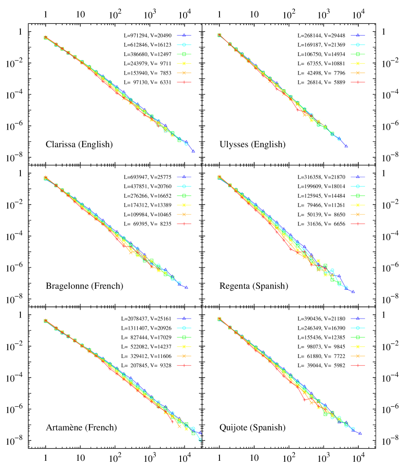
Figure 1: Density of word frequencies $D_{L}(n)$ ($y$-axis) against absolute frequency $n$ ($x$-axis), for six different books, taking text length $L=L_{\text{tot}}/10$, $L_{\text{tot}}/10^{4/5}$, $L_{\text{tot}}/10^{3/5}$, $\dots$, $L_{\text{tot}}$. The slope seems to decrease with text length.

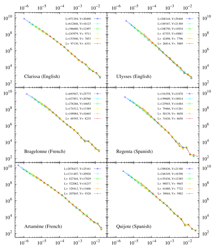
Figure 2: Rescaled densities $LV_{L}D_{L}(n)$ ($y$-axis) against relative frequency $n/L$ ($x$-axis), for the same books and fractions of text as in Fig. 1. The rescaled densities collapse onto a single function, independently of the value of $L$, validating our proposed scaling form for $D_{L}(n)$ [Eq. (2)] and making it clear that the decrease of the log-log slope with $L$ is not a consequence of a genuine change in the scaling properties of the distribution.

However, a scaling analysis reveals an alternative picture. As suggested by Eq. (2), plotting $LV_{L}D_{L}(n)$ against $n/L$ for different values of $L$ yields a collapse of all the curves onto a unique $L-$independent function for each book, which represents the scaling function $g(x)$. Figure 2 shows this for the same books and parts of the books as in Fig. 1. The data collapse can be considered excellent, except for the smallest frequencies. For the largest $L$ the collapse is valid up to $n\simeq 3$ if we exclude La Regenta, which only collapses for about $n\geq 6$. So, our scaling hypothesis is validated, independently of the particular shape that $g(x)$ takes. Note that $g(x)$ is independent of $L$ but not the book, i.e., each book has its own $g(x)$, different from the rest. In any case, we observe a slightly convex shape in log-log space, which leads to the rejection of the power-law hypothesis for the whole range of frequencies. Nevertheless, the data does not show any clear parametric functional form. A double power law, a stretched exponential, a Weibull, or a lognormal tail could be fit to the distributions. This is not incompatible with the fact that the large $n$ tail can be well fit by a power law (the Zipf’s law), for more than 2 orders of magnitude Corral et al. (2013).

Things turn out to be somewhat different after the lemmatization process. The scaling ansatz is still clearly valid for the frequency distributions, see Fig. 3, but with a different kind of scaling function $g(x)$, with a more defined characteristic shape, due to a more pronounced log-log curvature or convexity. In fact, close examination of the data leads us to conclude that the lemmatization process enhances the goodness of the scaling approximation, specially in the low-frequency zone. It could be reasoned that, as lemmatized texts have a significantly reduced vocabulary compared to the original ones, but the total length remains essentially the same, they are somehow equivalent to much longer texts, if one considers the length-to-vocabulary ratio. Although this matter needs to be further investigated, it supports the idea that our main hypothesis, the scale-invariance of the distribution of frequencies, holds more strongly for longer texts.

Due to the clear curvature of $g(x)$ in the lemmatized case, we go one step further and propose a concrete function to fit these data, namely,

$$g(x)=\frac{k}{x(a+x^{\gamma-1})}.$$ (3)

This function has two free parameters, $a$ and $\gamma$ (with $\gamma>1$ and $a>0$), and behaves as a double power law, that is, for large $x$, $g(x)\sim x^{-\gamma}$ (we still have Zipf’s law), while for small $x$, $g(x)\sim x^{-1}$. The transition point between both power-law tails is determined by $a$ (more precisely, by $a^{\frac{1}{\gamma-1}}$), and $k$ is fixed by normalization. But an important issue is that it is not $g(x)$ which is normalized to one but $D_{L}(n)$. We select a power-law with exponent one for small $x$ for three reasons: first, in order to explore an alternative to the power law in the $V_{L}$ versus $L$ relation (which is not clearly supported by the data, see next section); second, to allow for a better comparison of our results and those of Ref. Bernhardsson et al. (2009); third, to keep the number of parameters minimum. Thus, we do not look for the most accurate fit but for the simplest description of the data.

Then, defining $n_{a}=a^{\frac{1}{\gamma-1}}L$, the corresponding word-frequency density (or, more properly, lemma-frequency density, or type-frequency density) turns out to be

$$D_{L}(n)\propto\frac{1}{n\left(1+(n/n_{a})^{\gamma-1}\right)},$$ (4)

with $n_{a}$ the scale parameter (recall that the scale parameter of $g(x)$ was $a^{\frac{1}{\gamma-1}}$).

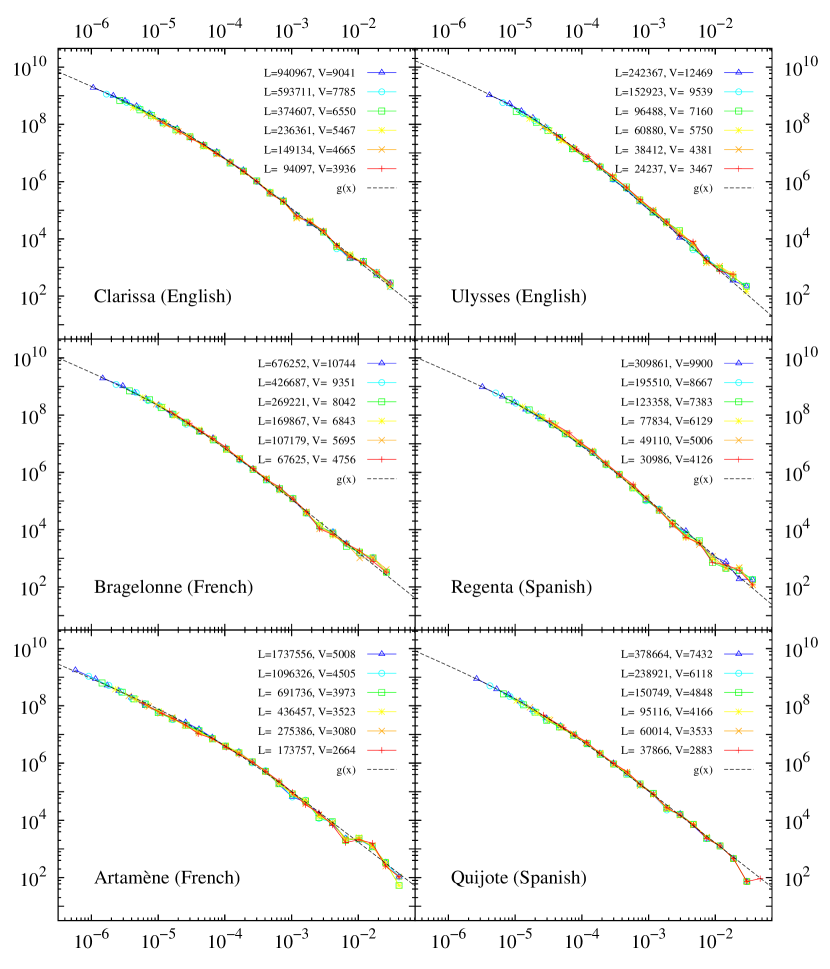
Figure 3: Same rescaled distributions as in previous figure ($LV_{L}D_{L}(n)$ versus $n/L$), but for the frequencies of lemmas. The data collapse guarantees the fulfillment of the scaling law also in this case. The fit resulting from the double power-law distribution, Eq. (3), is also included.

The data collapse in Fig. 3 and the good fit imply that the Zipf-like exponent $\gamma$ does not depend on $L$, but the transition point between both power laws, $n_{a}$, obviously does. Hence, as $L$ grows the transition to the $\sim n^{-\gamma}$ regime occurs at higher absolute frequencies, given by $n_{a}$, but fixed relative frequencies, given by $a^{\frac{1}{\gamma-1}}$. In Table 2 we report the fitted parameters for all seven books, obtained by maximum likelihood estimation of the frequencies of the whole books, as well as Monte Carlo estimates of their uncertainties. We have confirmed the stability of $\gamma$ fitting only a power-law tail from a fixed common relative frequency, for different values of $L$ Corral et al. (2013).

title	$n_{a}\pm\sigma_{n_{a}}$	$\gamma\pm\sigma_{\gamma}$	$a\pm\sigma_{a}$
Artamène(l)	$129.7\pm 12.6$	$1.807\pm 0.026$	$(4.65\pm 0.91)\cdot 10^{-4}$
Clarissa(l)	$32.70\pm 2.17$	$1.864\pm 0.021$	$(1.40\pm 0.24)\cdot 10^{-4}$
Don Quijote(l)	$7.91\pm 0.75$	$1.827\pm 0.020$	$(1.35\pm 0.22)\cdot 10^{-4}$
La Regenta(l)	$9.45\pm 0.66$	$1.983\pm 0.021$	$(3.68\pm 0.62)\cdot 10^{-5}$
Bragelonne(l)	$14.56\pm 1.23$	$1.866\pm 0.018$	$(9.10\pm 1.37)\cdot 10^{-5}$
Moby-Dick(l)	$8.21\pm 0.53$	$2.050\pm 0.024$	$(2.42\pm 0.47)\cdot 10^{-5}$
Ulysses(l)	$5.38\pm 0.31$	$2.020\pm 0.017$	$(1.79\pm 0.28)\cdot 10^{-5}$

Table 2: Values of the parameters $n_{a},\gamma$, and $a$ for the lemmatized versions (indicated with the superscript $l$) of the seven complete books. The fits are performed numerically through maximum likelihood estimation, while the standard deviations come from Monte Carlo simulations, see Appendix B.

Regarding the low-frequency exponent, one could find a better fit if the exponent was not fixed to be one; however, our data does not allow this value to be well constrained. A more important point is the influence of lemmatization errors in the characteristics of the low-frequency regime. Although the tools we use are rather accurate, rare words are likely to be assigned a wrong lemma. This limitation is intrinsic to current computational tools and has to be considered as a part of the lemmatization process. Nevertheless, the fact that the behavior at low frequencies is robust in front of a large variation in the percentage of lemmatization errors implies that our result is a genuine consequence of the lemmatization. See Appendix A for more details.

Although double power laws have been previously fit to rank-frequency plots for unlemmatized multi-author corpora Ferrer i Cancho and Solé (2001); Gerlach and Altmann (2013); Petersen et al. (2012), the resulting exponents for large ranks (low frequencies) are different than the ones obtained for our lemmatized single-author texts. Note that Ref. Gerlach and Altmann (2013) also proposed that the crossover between both power laws happened for a constant number of types, around 7900, independently of corpus size. This corresponds indeed to $r=7900$ and therefore, from Eq. (1), to a fixed relative frequency. This is certainly in agreement with our results, supporting the hypothesis that rank-frequency plots and frequency distributions are stable in terms of relative frequency.

IV An asymptotic approximation of Heaps’ law

Coming back to our scaling ansatz, Eq. (2), the normalization of $D_{L}(n)$ will allow us to establish a relationship between the word-frequency distribution and the growth of the vocabulary with text length. In the continuous approximation,

$$1=\int_{1}^{\infty}D_{L}(n)dn=\frac{1}{V_{L}}\int_{1}^{\infty}g(n/L)\frac{dn}{L}=\frac{1}{V_{L}}\int_{1/L}^{\infty}g(x)dx=\frac{1}{V_{L}}G\left(\frac{1}{L}\right),$$

where we have used the previous relation $g(x)=-G\hskip 1.99168pt^{\prime}(x)$, and have additionally imposed $G(\infty)\equiv 0$, for which it is necessary that $g(x)$ decays faster than a power law with exponent one. So,

$$V_{L}=G\left(\frac{1}{L}\right).$$ (5)

This just means, compared to Eq. (1), that the number of types with relative frequency greater or equal than $1/L$ is the vocabulary size $V_{L}$, as this is the largest rank for a text of length $L$. It is important to notice the difference between saying that $G_{L}(1/L)=V_{L}$, which is a trivial statement, and stating that $G(1/L)=V_{L}$, which provides a link between Zipf’s and Heaps’ law, or, more generally, between the distribution of frequencies and the vocabulary growth, by approximating the latter by the former. The quality of such an approximation will depend, of course, on the goodness of the scale-invariance approximation. In the usual case of a power-law distribution of frequencies extending to the lowest values, $g(x)\propto 1/x^{\gamma}$, with $\gamma>1$, then $G(x)\propto 1/x^{\gamma-1}$, which turns into Heaps’ law, $V_{L}\propto L^{\alpha}$, with $\alpha=\gamma-1$, in agreement with previous research Mandelbrot (1961); Kornai (2002); Lü et al. (2010); Serrano et al. (2009); Bernhardsson et al. (2009).

However, this power-law growth of $V_{L}$ with $L$ is not what is observed in texts, in general. Due to the accurate fit that we can achieve for lemmatized texts, we can explicitly derive an asymptotic expression for $V_{L}$ given our proposal for $g(x)$. As we have just shown, $g(x)$ is not normalized to one, rather, $\int_{1/L}^{\infty}g(x)dx=V_{L}$. Hence, substituting $g(x)$ from Eq. (2) and integrating,

$$V_{L}= \int_{1/L}^{\infty}\frac{k}{x(a+x^{\gamma-1})}dx=\frac{k}{a}\int_{1/L}^{\infty}\frac{ax^{-\gamma}}{ax^{1-\gamma}+1}dx=$$

$$= \frac{k}{a(1-\gamma)}\ln(ax^{1-\gamma}+1)\Bigr{|}_{1/L}^{\infty}=\frac{k}{a(\gamma-1)}\ln(aL^{\gamma-1}+1).$$ (6)

In this case $V_{L}$ is not a power law, and behaves asymptotically as $\propto\ln L$. This is a direct consequence of our choice for the exponent 1 in the left-tail of $g(x)$. Indeed, it seems clear that the vocabulary growth curve greatly deviates from a straight line in log-log space, for it displays a prominent convexity, see Fig. 4 as an example. Nevertheless, the result from Eq. (6) is not a good fit either, due to a wrong proportionality constant. This is caused by the continuous approximation in Eq. (6).

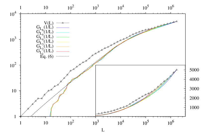
Figure 4: The actual curve $V_{L}$ (solid black with triangles) for the lemmatized version of the book Artamène, together with the curves $V_{L}=G(1/L)$ obtained by using the empirical inverse of the rank-frequency plot, $r=G(n/L)$, with $L_{i}=L_{\text{tot}}/10^{(6-i)/5}$ (colors), and the analytical expression Eq. (7) with parameters determined from the fit of $D_{L_{\text{tot}}}(n)$, Eq. (6) (dashed black).

For an accurate calculation of $V_{L}$ we must treat our variables as discrete and compute discrete sums rather than integrals. In the exact, discrete treatment of $D_{L}(n)$, equation (6) must be rewritten as

$$V_{L} =G\left(\frac{1}{L}\right)=G\left(\frac{L_{\text{tot}}/L}{L_{\text{tot}}}\right)=\sum_{n\geq L_{\text{tot}}/L}\frac{g(n/L_{\text{tot}})}{L_{\text{tot}}}=$$

$$=\frac{1}{L_{\text{tot}}}\sum_{n\geq L_{\text{tot}}/L}\frac{k}{\left(\frac{n}{L_{\text{tot}}}\right)\left(a+\left(\frac{n}{L_{\text{tot}}}\right)^{\gamma-1}\right)}$$ (7)

where we have used the fact that $S_{L_{\text{tot}}}(n^{\prime})=\sum_{n\geq n^{\prime}}D_{L_{\text{tot}}}(n)$, with $n^{\prime}=L_{\text{tot}}/L$ (notice that in the discrete case, $g(x)\neq-G^{\prime}(x)$). This is consistent with the fact that, indeed, the maximum likelihood parameters $\gamma$ and $a$ have been computed assuming a discrete probability function (see Appendix B), and so has the normalization constant. We would like to stress that no fit is performed in Figure 4, that is, the constant $k$ in $g(x)$ is directly derived from the normalizing constant of $D_{L}(n)$, and depends only on $\gamma$ and $a$.

V Conclusions

In summary, we have shown that, contrary to claims in previous research Baayen (2001); Powers (1998); Bernhardsson et al. (2009), Zipf’s law in linguistics is extraordinarily stable under changes in the size of the analyzed text. A scaling function $g(x)$ provides a constant shape for the distribution of frequencies of each text, $D_{L}(n)$, no matter its length $L$, which only enters into the distribution as a scale parameter and determines the size of the vocabulary $V_{L}$. The apparent size-dependent exponent found previously seems to be an artifact of the slight convexity of $g(x)$ in a log-log plot, which is more clearly observed for very small values of $x$, accessible only for the largest text lengths. Moreover, we find that in the case of lemmatized texts the distribution can be well described by a double power law, with a large-frequency exponent $\gamma$ that does not depend on $L$, and a transition point $n_{a}$ that scales linearly with $L$. The small-frequency exponent is different than the ones reported in Refs. Ferrer i Cancho and Solé (2001); Gerlach and Altmann (2013) for non-lemmatized corpora. Further, the stability of the shape of the frequency distribution allows one to predict the growth of vocabulary size with text length, resulting in a generalization of the popular Heaps’ law.

The robustness of Zipf-like parameters under changes in system size opens the way to more practical applications of word statistics. In particular, we provide a consistent way to compare statistical properties of texts with different lengths Baixeries et al. (2013). Another interesting issue would be the application of the same scaling methods to other fields in which Zipf’s law has been proposed to hold, as economics and demography, for instance.

Appendix A Lemmatization

To analyze the distribution of frequencies of lemmas, the texts needed to be lemmatized. To manually lemmatize the words would have exceeded the possibilities of this project, so we proceeded to automatic processing with standard computational tools: FreeLing FreeLing for Spanish and English and TreeTagger Schmid (1994) for French. The tools carry out the following steps:

1. Tokenization: Segmentation of the texts into sentences and sentences into words (tokens).

2. Morphological analysis: Assignment of one or more lemmas and morphological information (tag) to each token. For instance, found in English can correspond to the past tense of the verb find or to the base form of the verb found. At this stage, both are assigned whenever the word form found is encountered.

3. Morphological disambiguation: An automatic tagger assigns the single most probable lemma and tag to each word form, depending on the context. For instance, in I found the keys the tagger would assign the lemma find to the word found, while in He promised to found a hospital, the lemma found would be preferred.

All these steps are automatic, such that errors are introduced at each step. However, the accuracy of the tools is quite high (e.g., around 95-97% at the token level for morphological disambiguation), so a quantitative analysis based on the results of the automatic process can be carried out. Also note that step 2 is based on a pre-existing dictionary (of words, not of lemmas, also called a lexicon): only the words that are in the dictionary are assigned a reliable set of morphological tags and lemmas. Although most of the tools used heuristically assign tag and/or lemma information to words that are not in the dictionary, we only count tokens of lemmas for which the corresponding word types are found in the dictionary, so as to minimize the amount of error introduced by the automatic processing. This comes at the expense of losing some data. However, the dictionaries have quite a good coverage of the vocabulary, particularly at the token level, but also at the type level (see Table 3). The exceptions are Ulysses, because of the stream of consciousness prose, which uses many non-standard word forms, and Artamène, because 17th century French contains many word forms that a dictionary of modern French does not include.

Table 3: Coverage of the vocabulary by the dictionary in each language, both at the type and at the token level. Remember that we distinguish between a word type (corresponding to its orthographic form) and its tokens (actual occurrences in text).

title	types	tokens
Clarissa	68.0 %	96.9 %
Moby-Dick	70.8 %	94.7 %
Ulysses	58.6 %	90.4 %
Don Quijote	81.3 %	97.0 %
La Regenta	89.5 %	97.9 %
Artamène	43.6 %	83.6 %
Bragelonne	89.8 %	97.5 %
Seitsemän v.	89.8 %	95.4 %
Kevät ja t.	96.2 %	98.3 %
Vanhempieni r.	96.5 %	98.5 %
average	78.4 %	95.0 %

Appendix B Maximum likelihood fitting

The fitted values of Table 2 have been obtained by maximum-likelihood estimation (MLE). This well-known procedure consists firstly in computing the log-likelihood function $\mathcal{L}$, which in our case reads

$$\mathcal{L}=\frac{1}{V_{L}}\sum_{i=1}^{V_{L}}\ln D_{L}(n_{i})=\ln K-\frac{1}{V_{L}}\sum_{i=1}^{V_{L}}\ln\left(n_{i}(b+n_{i}^{\gamma-1})\right)$$

with $n_{i}$ the $V_{L}$ values of the frequency and the normalization constant $K$ in the discrete case equal to

$$K=\left[\sum_{n=1}^{n_{\max}}\frac{1}{n(b+n^{\gamma-1})}\right]^{-1}.$$

Note that we have reparameterized the distribution compared to the main text, introducing $b=n_{a}^{\gamma-1}=aL^{\gamma-1}$. Then, $\mathcal{L}$ is maximized with respect to the parameters $\gamma$ and $b$; this has been done numerically using the simplex method Press et al. (1992). The error terms $\sigma_{\gamma}$ and $\sigma_{b}$, representing the standard deviation of each estimator, are computed from Monte Carlo simulations: From the resulting maximum-likelihood parameters $\gamma^{*}$ and $b^{*}$, synthetic data samples are simulated, and the MLE parameters of these samples are calculated in the same way; their fluctuations yield $\sigma_{\gamma}$ and $\sigma_{b}$. We stress that no continuous approximation has been made, that is, the simulated data follows the discrete probability function $D_{L}(n)$ (this is done using the rejection method, see Ref. Devroye (1986); Corral et al. (2013) for details for a similar case). In a summarized recipe, the procedure simply is:

1. Numerically compute the MLE parameters, $\gamma^{*}$ and $b^{*}$.

2. Draw $M$ datasets, each of size $V_{L}$, from the discrete probability function $D_{L}(n;\gamma^{*},b^{*})$.

3. For each dataset $m=1\dots M$, compute the MLE parameters $\gamma^{m},b^{m}$.

4. Compute the standard deviations $\sigma_{\gamma}$ and $\sigma_{b}$ of the sets $\{\gamma^{m}\}_{m=1}^{M}$ and $\{b^{m}\}_{m=1}^{M}$.

The standard deviations of $n_{a}$ and $a$ are computed in the same way using their relationship to $b$ and $\gamma$.