Penalized Likelihood and Bayesian Function Selection in Regression Models

Abstract

Challenging research in various fields has driven a wide range of methodological advances in variable selection for regression models with high-dimensional predictors. In comparison, selection of nonlinear functions in models with additive predictors has been considered only more recently. Several competing suggestions have been developed at about the same time and often do not refer to each other. This article provides a state-of-the-art review on function selection, focusing on penalized likelihood and Bayesian concepts, relating various approaches to each other in a unified framework. In an empirical comparison, also including boosting, we evaluate several methods through applications to simulated and real data, thereby providing some guidance on their performance in practice.

Key-words: generalized additive model, regularization, smoothing, spike and slab priors

1 Introduction

Challenging substantive research questions and technological innovations, beginning in molecular life sciences, stimulated a revival of methodological and applied research for selection of influential components in regression models. There exists now a vast literature on variable selection in linear regression models

$$y_{i}=\beta_{0}+\beta_{1}x_{i1}+\ldots+\beta_{p}x_{ip}+\epsilon_{i}=\eta_{i}^{\operatorname{lin}}+\epsilon_{i},\quad i=1,\ldots,n,$$ (1)

as well as in generalized linear models or hazard rate models, with high-dimensional linear predictor $\eta_{i}^{\operatorname{lin}}$, where $p$ is (very) large compared to the sample size $n$.

In comparison, corresponding research on function selection in additive models

$$y_{i}=\beta_{0}+f_{1}(x_{i1})+\ldots+f_{p}(x_{ip})+\epsilon_{i}=\eta_{i}^{\operatorname{add}}+\epsilon_{i}$$ (2)

is more recent and still comparably sparse, especially so for non-Gaussian models with additive predictors $\eta_{i}^{\operatorname{add}}$, possibly including further components such as linear effects and interaction terms.

The following related issues are of interest in function selection: Should a function $f_{j}(x_{j})$ be included in the predictor at all? Because functions are usually centered around zero, we therefore want to know whether $f_{j}(x_{j})$ differs significantly from zero. Moreover, we are often interested whether the effect is linear, that is $f_{j}(x_{j})=\beta_{j}x_{j}$ or nonlinear, that is, does $f_{j}(x_{j})$ differ significantly from a straight line? Is the approximation of the regression function through an additive predictor good enough or do we have to incorporate varying coefficient terms, such as $f_{1}(x_{1})x_{2}$, or interactions such as $f_{12}(x_{1},x_{2})$?

The aims of this article are as follows: We provide a state-of-the-art survey on recent advances in function selection. Our focus is on penalized least squares or likelihood methods and on Bayesian concepts, in particular based on selection indicators and spike-and-slab priors. We sketch - mostly asymptotic - results on model selection consistency, convergence rates or oracle properties, as far as they are available. To explore and to illustrate performance in finite sample situations, we compare and evaluate several methods through application to simulated and real benchmark data. Naturally, usable software implementation has been a key criterion for including a selection method into this empirical evaluation. This is the first empirical comparison of several recent methods for function selection and provides guidance on their performance in practice.

Most frequentist and Bayesian approaches for function selection are based on or motivated from variable selection in regression models with high-dimensional linear predictors as in (1). Very popular penalization methods for variable selection are the Lasso [Tibshirani, 1996], the SCAD penalty [Fan and Li, 2001], and modifications such as the adaptive Lasso [Zou, 2006], the groupLasso [Yuan and Lin, 2006] and the groupSCAD [Wang et al., 2007]. Another branch is boosting [Bühlmann and Yu, 2003, Bühlmann and Hothorn, 2007], which we include as a further competitor in our empirical analyses since it is applicable to a wide range of regression models and is implemented in the R package mboost [Hothorn et al., 2012].

Bayesian variable selection in linear predictors is often based on spike-and-slab priors for single regression coefficients and has been most extensively discussed for the classical linear model (1), see George and McCulloch [1993, 1997]. The basic idea is that each coefficient $\beta_{l}$ is modeled as having come either from a distribution with most (or all) of its mass concentrated around zero (the ’spike’), or from a comparably diffuse distribution (the ’slab’). A closely related concept is to introduce selection indicator variables for coefficients being zero or non-zero [Smith and Kohn, 1996]. Instead of placing spike-and-slab priors directly on regression coefficients, Ishwaran and Rao [2005] assume a spike-and-slab prior for the variance of (conditionally) Gaussian priors. This concept is conveniently extended to generalized linear models, see Fahrmeir et al. [2010]. In a recent review paper, O’Hara and Sillanpää [2009] compare several Bayesian variable selection methods for linear models; see also Fahrmeir and Kneib [2011, Section 4.5.3].

The common feature of penalization methods for function selection is to place a penalty on certain norms of functional components or associated blocks of basis function coefficients. The penalty term usually enforces sparseness or smoothness of regression functions, but both properties are also related to each other through the choice of the function space. Lin and Zhang [2006] proposed the component selection and smoothing operator (COSSO) in additive smoothing spline ANOVA models, with extensions to exponential family responses in Zhang and Lin [2006] and to hazard regression in Leng and Zhang [2006]. Ravikumar et al. [2009] enforce sparsity in additive models by imposing a penalty on the empirical $L_{2}$-norm of functional components. Meier et al. [2009] incorporate an additional smoothness penalty and Radchenko and James [2010] impose a further $L_{2}$-norm penalty to obtain sparse hierarchical structures in models with two-way functional interactions. All these methods include only one global penalty parameter to enforce sparseness of main effects, or a second one to control the amount of smoothness of main effects or hierarchical structures in two-way interaction models. This leads to a tendency to oversmooth nonzero functional components in order to set unimportant functions to zero. Motivated by the adaptive groupLasso, Storlie et al. [2011] propose the adaptive COSSO (ACOSSO) to penalize each functional component in additive models differently so that more flexibility is obtained for functional components with more curvature while shrinking unimportant components more heavily to zero. Zhang et al. [2011b] extend the adaptive COSSO by decomposing nonlinear functions into a linear part and a nonlinear deviation. A similar adaptive groupLasso approach is studied in Huang et al. [2010]. Instead of penalizing directly the norms of basis function coefficient vectors, leading to groupLasso-type penalties, Xue [2009, for additive models] and Wang et al. [2007, for varying coefficient models], insert norms into the SCAD penalty, leading to groupSCAD-type penalties.

Belitz and Lang [2008] propose a simple and computationally efficient method for simultaneous estimation and selection in (generalized) additive models based on the quadratic P-spline penalty in combination with an extended backfitting algorithm. In a double penalty approach, Marra and Wood [2011] decompose the quadratic smoothing spline penalty for generalized additive models into two terms corresponding to the null space, e.g. linear functions, and the penalty range space, e.g. cubic spline deviations from linear functions, shrinking both of them to zero. A related idea has been suggested in Avalos et al. [2007] for additive models, shrinking linear functions to zero in Lasso-type fashion.

While most penalization methods have been primarily developed for additive models, boosting approaches are also available for more general semiparametric predictors and non-Gaussian models, see e.g. Tutz and Binder [2006] and Kneib et al. [2009].

Bayesian function selection is mostly based on introducing spike-and-slab priors with a point mass at zero for blocks of basis function coefficients or, equivalently, indicator variables for functions being zero or nonzero. Wood et al. [2002] and Yau et al. [2003] describe implementations using a data-based prior that requires two MCMC runs, a pilot run to obtain a data-based prior for the “slab” part and a second one to estimate parameters and select model components. Panagiotelis and Smith [2008] combine this indicator variable approach with partially improper Gaussian priors, as for basis coefficients of Bayesian P-splines, in high-dimensional additive models. They suggest several sampling schemes that dominate the scheme in Yau et al. [2003]. A more general approach based on double exponential regression models that also allows for flexible modeling of the dispersion is described by Cottet et al. [2008]. They use a reduced rank representation of cubic smoothing splines with a very small number of basis functions to model the smooth terms in order to reduce the complexity of the fitted models, and, presumably, to avoid mixing problems. Reich et al. [2009] consider a Gaussian functional ANOVA model with (conditionally) conjugate Gaussian process priors for functions. To perform function selection, they impose a spike-and-slab prior on variances of Gaussian processes, with a point mass at zero for the spike and a half-Cauchy prior for the slab. It seems difficult, however, to extend it to non-Gaussian regression models.

A novel spike-and-slab prior structure for function selection in the broad class of structured additive regression models for Gaussian and discrete responses is proposed in Scheipl [2011a], Scheipl et al. [2012] and implemented in the R package spikeSlabGAM [Scheipl, 2011b].

2 Penalized least squares and likelihood-based function selection

2.1 General concept

Let $\boldsymbol{y}=(y_{1},\ldots,y_{n})^{{}^{\prime}}$ denote the vector of all responses, $\boldsymbol{\eta}=(\eta_{1},\ldots,\eta_{n})^{{}^{\prime}}$ the vector of corresponding predictor values, and $\boldsymbol{f}_{j}=(f_{j}(x_{1j}),\ldots,f_{j}(x_{nj}))^{{}^{\prime}}$ the vector of function evaluations of a function $f_{j}(x_{j})$. All penalization methods measure the fit of a regression model by some loss function $\operatorname{loss}(\boldsymbol{y},\boldsymbol{\eta})$ or equivalently through a utility function $\operatorname{utility}(\boldsymbol{y},\boldsymbol{\eta})=-\operatorname{loss}(\boldsymbol{y},\boldsymbol{\eta})$.

The $L_{2}$-loss

$$\operatorname{loss}(\boldsymbol{y},\boldsymbol{\eta})=||\boldsymbol{y}-\boldsymbol{\eta}||^{2}$$

i.e., the squared Euclidian distance between $\boldsymbol{y}$ and $\boldsymbol{\eta}$, is commonly used for additive models $\boldsymbol{y}=\boldsymbol{\eta}^{\operatorname{add}}+\boldsymbol{\epsilon}$ and extensions including a linear predictor $\boldsymbol{\eta}^{\operatorname{lin}}$ or interaction terms. Sometimes the empirical $L_{2}$-loss $||\boldsymbol{y}-\boldsymbol{\eta}||^{2}/n$ is considered as a slight modification. For Gaussian i.i.d. errors the $L_{2}$-loss coincides with the negative log-likelihood, up to an additive constant. The $L_{2}$-loss is also considered for non-Gaussian errors with distributions with similar shapes, but then it is only a (negative) quasi-log-likelihood. To improve efficiency, one may consider a weighted $L_{2}$-loss, with weights proportional to the inverse standard deviations. For non-Gaussian responses with exponential family distributions, in particular binary, categorical or count responses, the negative log-likelihood

$$\operatorname{loss}(\boldsymbol{y},\boldsymbol{\eta})=-\operatorname{l}(\boldsymbol{y},\boldsymbol{\eta})$$

is a more natural choice. For Cox-type hazard regression models or quasi-likelihood models the loss is defined by the (negative) partial log-likelihood or some pseudo-log-likelihood.

To regularize estimation of high-dimensional regression models and to enforce sparseness through component selection and/or smoothness of functions, a penalty function $\operatorname{pen}(\boldsymbol{\eta})$ is introduced, including one or more tuning parameters $\lambda$ to control the amount of penalization. For models with an additive predictor (2), the penalty is a sum of penalties for each function

$$\operatorname{pen}(\boldsymbol{\eta})=\sum_{j=1}^{p}\operatorname{pen}_{j}(\boldsymbol{f}_{j}),$$

where each penalty term $\operatorname{pen}_{j}(\boldsymbol{f}_{j})$ includes one (or two) tuning parameter common to all of them, or separate, in case of tensor product terms possibly multi-dimensional, tuning parameters $\boldsymbol{\lambda}_{j}$ for each of them. We distinguish between sparseness and smoothness penalties. Sparseness penalties are constructed to shrink (suitable norms of) functions to zero, deleting “unimportant” functions. Smoothness is - hopefully - obtained as a by-product, e.g. through the choice of a suitable space of smooth functions. Smoothness penalties explicitly encourage the fitting of smooth functions. Modifications of well-known smoothing spline penalized or regression spline approaches are required, however, to encourage sparseness of predictors. Section 2.2 describes sparseness penalties in more detail, while Section 2.3 deals with smoothness penalties or a combination of both types.

The ultimate goal is to (simultaneously) estimate and select functions $\boldsymbol{f}=(f_{1},\ldots,f_{j},\ldots)$ by minimizing the penalized loss

$$\operatorname{loss}(\boldsymbol{y},\boldsymbol{\eta})+\operatorname{pen}(\boldsymbol{\eta})\rightarrow\underset{\boldsymbol{f}\in\mathcal{F}}{\operatorname{min}}$$

where $\mathcal{F}$ is a prespecified suitable function space. Tuning parameters are assumed to be fixed or known in this minimization problem and are estimated by minimizing additional criteria, in particular cross-validation, information criteria such as (modifications of) AIC, BIC, and Mallows $\text{C}_{p}$, or (restricted) marginal likelihood (REML).

In almost all approaches considered in Sections 2.2 and 2.3, the function space $\mathcal{F}_{j}$ for each function $f_{j}$ is a linear space defined through basis functions $B_{jk}(x),\;k=1,2,\ldots$, such as the space of polynomial splines equipped with a B-spline basis. Then

$$f_{j}(x)=\sum_{k}\beta_{jk}B_{jk}(x)$$ (3)

and the vector $\boldsymbol{f}_{j}$ of function evaluations can be expressed as

$$\boldsymbol{f}_{j}=\boldsymbol{X}_{j}\boldsymbol{\beta}_{j}$$ (4)

with basis function values $B_{jk}(x_{ij})$ as elements of the design matrix $\boldsymbol{X}_{j}$. Then the penalized loss can be expressed as

$$\operatorname{loss}(\boldsymbol{y},\boldsymbol{\beta})+\operatorname{pen}(\boldsymbol{\beta})\rightarrow\underset{\boldsymbol{\beta}}{\operatorname{min}},$$

where $\boldsymbol{\beta}$ is the vector of all basis function coefficients. For an additive model (2) and an $L_{2}$-loss, we obtain the penalized least squares criterion

$$\operatorname{PLS}(\boldsymbol{\beta})=||\boldsymbol{y}-\mathbf{1}\beta_{0}-\sum_{j=1}^{p}\boldsymbol{X}_{j}\boldsymbol{\beta}_{j}||^{2}+\sum_{j=1}^{p}\operatorname{pen}_{j}(\boldsymbol{\beta}_{j})\rightarrow\underset{\beta_{0},\boldsymbol{\beta}}{\operatorname{min}}.$$ (5)

with $\mathbf{1}=(1,\ldots,1)^{{}^{\prime}}$ denoting a vector of ones. To guarantee identifiability, appropriate constraints have to be introduced. In particular, we have to assume non-concurvity of the functions and ensure that each function estimate is centered around zero.

Many function selection penalties are based on or related to the groupLasso. Yuan and Lin [2006] introduced it for linear models as an extension of the Lasso for selecting groups of coefficients $\boldsymbol{\beta}_{j}$ associated with factor variables or a polynomial function of a continuous covariate. The groupLasso estimator is defined as the solution to

$$||\boldsymbol{y}-\mathbf{1}\beta_{0}-\sum_{j=1}^{p}\boldsymbol{X}_{j}\boldsymbol{\beta}_{j}||^{2}+\lambda\sum_{j=1}^{p}||\boldsymbol{\beta}_{j}||_{\boldsymbol{K}_{j}}\rightarrow\underset{\beta_{0},\boldsymbol{\beta}_{1},\ldots,\boldsymbol{\beta}_{p}}{\operatorname{min}}.$$ (6)

where the design matrix $\boldsymbol{X}_{j}$ corresponds to the $j$th factor. After centering covariates and responses, the unpenalized intercept term may be omitted for simplicity. The norms in the groupLasso penalty are defined by

$$||\boldsymbol{\beta}_{j}||_{\boldsymbol{K}_{j}}=(\boldsymbol{\beta}_{j}^{{}^{\prime}}\boldsymbol{K}_{j}\boldsymbol{\beta}_{j})^{1/2},$$

where $\boldsymbol{K}_{j}$ is a $d_{j}\times d_{j}$ positive (semi-)definite matrix $\boldsymbol{K}_{j}$, $d_{j}=\operatorname{dim}(\boldsymbol{\beta}_{j})$. For $d_{j}=1,\quad j=1,\ldots,p$, the groupLasso reduces to the usual Lasso. For $\boldsymbol{K}_{j}=\boldsymbol{I}_{dj}$, the norm reduces to the Euclidian norm $||\boldsymbol{\beta}_{j}||$. To scale for different dimensions of the coefficient vectors, $\boldsymbol{K}_{j}=d_{j}\boldsymbol{I}_{dj}$ may be chosen, so that $||\boldsymbol{\beta}_{j}||_{\boldsymbol{K}_{j}}$ reduces to $\sqrt{d_{j}}||\boldsymbol{\beta}_{j}||$. Yuan and Lin [2006] discuss shrinkage properties of the groupLasso and suggest a coordinate-wise algorithm for estimating the coefficients. Solution paths look similar as for the Lasso: Depending on the shrinkage parameter $\lambda$, $\hat{\boldsymbol{\beta}}_{j}$ may be exactly zero and the corresponding group of variables is removed from the model.

Conceptually, the groupLasso is easily extended to high-dimensional generalized linear models: The $L_{2}$-loss has to be replaced by the negative log-likelihood of a generalized linear model, e.g. a logit model, see Meier et al. [2008]. However, parameter estimation becomes more demanding. An implementation can be found in the R-package grplasso [Meier, 2009].

In analogy, the SCAD penalty of Fan and Li [2001] can be extended to a groupSCAD penalty by inserting some norm $||\boldsymbol{\beta}_{j}||_{\boldsymbol{K}_{j}}$ into the (scalar) argument of the SCAD penalty. This seems promising, at least from an asymptotic point of view, because the SCAD selector possesses the oracle property, in contrast to the Lasso selector.

2.2 Sparseness penalties

Ravikumar et al. [2009] develop function selection for sparse additive models based on the sparseness penalty

$$\operatorname{pen}(\boldsymbol{f}_{j})=\lambda\big{(}\frac{1}{n}\boldsymbol{f}_{j}^{{}^{\prime}}\boldsymbol{f}_{j}\big{)}^{1/2}=\lambda||\boldsymbol{f}_{j}||_{n}$$

where $||\boldsymbol{f}_{j}||_{n}$ is the empirical $L_{2}$-norm, and the functions are assumed to be centered around zero. Thus, the norm $||\boldsymbol{f}_{j}||_{n}$ penalizes deviations from zero and shrinks function to zero. The shrinkage parameter $\lambda$ is the same for all functions. To minimize the PLS criterion, they propose a “sparse” backfitting algorithm (SPAM) which works for any smoother, e.g. also for local linear or kernel smoothers. Thus, smoothness is considered implicitly. Their approach and parts of the algorithm can be seen as a “functional” version of the groupLasso. This becomes evident if functions are represented through basis functions. Then $\boldsymbol{f}_{j}=\boldsymbol{X}_{j}\boldsymbol{\beta}_{j}$ and the empirical $L_{2}$-norm becomes

$$\operatorname{pen}(\boldsymbol{\beta}_{j})=\lambda||\boldsymbol{\beta}_{j}||_{\boldsymbol{K}_{j}},\quad\boldsymbol{K}_{j}=\frac{1}{n}\boldsymbol{X}_{j}^{{}^{\prime}}\boldsymbol{X}_{j}$$ (7)

which is a groupLasso penalty.

Radchenko and James [2010] extend the sparse additive model by incorporating two-way interaction terms $f_{jl}$. They suggest the penalty function

$$\operatorname{pen}(\boldsymbol{\eta})=\lambda_{1}\sum_{j=1}^{p}(||\boldsymbol{f}_{j}||^{2}+\sum_{l=j+1}^{p}||\boldsymbol{f}_{jl}||^{2})^{1/2}+\lambda_{2}\sum_{j=1}^{p}\sum_{l=j+1}^{p}||\boldsymbol{f}_{jl}||,$$

where $||\cdot||$ is the usual $L_{2}$-norm. The first term penalizes all model terms, while the second term additionally discourages interaction terms to enter the model in order to support the hierarchical structure of main and interaction effects.

Huang et al. [2010] propose an adaptive groupLasso for additive models, with functions $f_{j}(x_{j})$ represented through B-splines. After centering the B-splines $B_{jk}(x)$ by redefining

$$B_{jk}(x):=B_{jk}-\bar{B}_{jk},\quad\bar{B}_{jk}(x)=\frac{1}{n}\sum_{i=1}^{n}B_{jk}(x_{ij})$$

(and centering responses around their mean), they suggest to estimate $\boldsymbol{\beta}_{j}$ through a PLS criterion with the adaptive groupLasso penalty

$$\operatorname{pen}(\boldsymbol{\beta}_{j})=\lambda w_{j}||\boldsymbol{\beta}_{j}||.$$ (8)

While the shrinkage parameter $\lambda$ is estimated through minimizing the BIC, the weights $w_{j}$ are determined in a first step via the groupLasso estimator, in analogy to the adaptive Lasso of Zou [2006] for linear models. Thus, another shrinkage parameter has to be estimated in this step. Because the adaptive Lasso possesses the oracle property, one may expect desirable properties for the adaptive groupLasso (see Section 2.4).

Xue [2009] and Wang et al. [2007] suggest a grouped version of the SCAD penalty for function selection in additive and varying coefficient models respectively. Functions $f_{j}(x_{j})$ are again represented through a B-spline expansion. Xue [2009] defines the groupSCAD penalty through

$$\operatorname{pen}(\boldsymbol{\beta}_{j})=p_{\lambda}(||\boldsymbol{\beta}_{j}||_{\boldsymbol{K}_{j}}),$$

where $\boldsymbol{K}_{j}=\boldsymbol{X}_{j}^{{}^{\prime}}\boldsymbol{X}_{j}/n$ as in (7), while Wang et al. [2007] insert the Euclidian norm $||\boldsymbol{\beta}_{j}||$ into the SCAD penalty of Fan and Li [2001]. It is given by

$$p_{\lambda}(w)=\begin{cases}\lambda|w|&\text{if }|w|\leq\lambda\\ -(w^{2}-2a\lambda|w|+\lambda^{2})&\text{if }\lambda<|w|<a\lambda\\ \frac{(a+1)\lambda^{2}}{2}&\text{if }|w|>a\lambda,\end{cases}$$

which is a quadratic spline with knots at $\lambda$ and $a\lambda$, with $a=3.7$ as a standard option. Because the SCAD selector in linear models possesses the oracle property, one may again expect desirable asymptotic properties for groupSCAD selectors (see Section 2.4).

2.3 Smoothness penalties

Smoothness penalties are well-known from representing and fitting smooth functions $f_{j}(x_{j})$ in additive and generalized additive models with predictors

$$\eta_{i}=\boldsymbol{x}_{0}^{{}^{\prime}}\boldsymbol{\beta}_{0}+\sum_{j=1}^{p}f_{j}(x_{ij})$$

through smoothing splines or penalized regression splines. Expressing splines by their basis function representations $\boldsymbol{f}_{j}=\boldsymbol{X}_{j}\boldsymbol{\beta}_{j}$ in (4), estimates $\boldsymbol{\hat{f}}_{j}$ and $\boldsymbol{\hat{\beta}}_{j}$ are obtained as the minimizers of

$$\operatorname{loss}(\boldsymbol{y},\boldsymbol{\beta})+\sum_{j=1}^{p}\operatorname{pen}_{j}(\boldsymbol{\beta}_{j})$$

where

$$\operatorname{pen}_{j}(\boldsymbol{\beta}_{j})=\lambda_{j}\boldsymbol{\beta}_{j}^{{}^{\prime}}\boldsymbol{K}_{j}\boldsymbol{\beta}_{j}=\lambda_{j}||\boldsymbol{\beta}_{j}||_{\boldsymbol{K}_{j}}^{2}.$$ (9)

The loss function is the $L_{2}$-norm for AMs and the negative exponential family log-likelihood for GAMs, and $\boldsymbol{K}_{j}$ are the penalty matrices of smoothing splines or P-splines measuring roughness of the fitted functions. Although the smoothness penalties (9) look similar to sparseness penalties, there are three important differences. First, the penalty matrices $\boldsymbol{K}_{j}$ are only positive semidefinite and the null space corresponds to functions which are not penalized. For the most common case of cubic splines, the null space consists of linear functions. This implies that functions will not be shrunk towards zero without some modification. Second, instead of the (semi-)norm $||\boldsymbol{\beta}_{j}||_{\boldsymbol{K}_{j}}$, the quadratic norm is used. Thus, $\boldsymbol{\hat{\beta}}_{j}$ is a Ridge-type but not a Lasso-type estimator. Third, the penalty terms have separate smoothness parameters $\lambda_{j}$ to allow for different degrees of smoothness of the various functions $f_{j}(x_{j}),\,j=1,\dots,p$. In contrast, all sparsity penalties have one (or two) common shrinkage parameters, leading to a tendency to oversmooth functions.

To circumvent the difficulty that smooth functions will in general not be estimated as zero even if they are nuisance functions, Marra and Wood [2011] impose an additional penalty on the null space. Let

$$\boldsymbol{K}_{j}=\boldsymbol{U}_{j}\boldsymbol{\Lambda}_{j}\boldsymbol{U}_{j}^{{}^{\prime}}$$

be the spectral decomposition of the smoothing matrix, with zero eigenvalues in $\boldsymbol{\Lambda}_{j}$ corresponding to the null space of $\boldsymbol{K}_{j}$. Then an extra penalty can be defined based on $\boldsymbol{K}_{j}^{*}=\boldsymbol{U}_{j}^{*}(\boldsymbol{U}_{j}^{*})^{{}^{\prime}}$, where $\boldsymbol{U}_{j}^{*}$ is the matrix of eigenvectors corresponding to the zero eigenvalues of $\boldsymbol{\Lambda}_{j}$. This allows to impose a double penalty

$$\lambda_{j}\boldsymbol{\beta}_{j}^{{}^{\prime}}\boldsymbol{K}_{j}\boldsymbol{\beta}_{j}+\lambda_{j}^{*}\boldsymbol{\beta}_{j}^{{}^{\prime}}\boldsymbol{K}_{j}^{*}\boldsymbol{\beta}_{j}$$

on each component $f_{j}$. By estimating $\lambda_{j}$ and $\lambda_{j}^{*}$ separately, a function $f_{j}$ can now be completely removed from the predictor. For the case of cubic smoothing splines, the first term penalizes deviations from a straight line and the second term penalizes straight but non-horizontal lines. This double penalty approach is implemented for GAMs in the R package mgcv [Wood, 2012].

A related idea has been considered by Avalos et al. [2007] for additive models. They impose a Lasso penalty on the coefficients of linear terms.

Belitz and Lang [2008] develop a computationally very efficient modification of backfitting for simultaneous component selection and model estimation. Their approach applies to the very broad class of structured additive regression, with continuous and discrete response as in generalized linear models. The additive predictor can include linear terms, smooth functions as well as interactions, spatial effects for geoadditive regression, and random effect terms for clustered or longitudinal data. Univariate functions are modelled through P-splines, two-way interactions through corresponding penalized tensor product-splines, spatial components through Gaussian Markov random fields, and (uncorrelated) random effects are assumed to be i.i.d. Gaussian. Each of these different types of “functions” $f_{j}$ is associated with a quadratic penalty

$$\operatorname{pen}(\boldsymbol{\beta}_{j})=\lambda_{j}||\boldsymbol{\beta}_{j}||_{\boldsymbol{K}_{j}}^{2},$$

where $\boldsymbol{K}_{j}$ depends on the different types of functions. For univariate smooth functions, $\boldsymbol{K}_{j}$ is the usual regression spline penalty matrix, a Markov random field precision matrix for spatial components, and an inverse correlation matrix for Gaussian random effects. Estimation and selection are carried out by modified backfitting for each of the components: At each step, a number of alternative smoothers is computed for a grid of smoothing parameters, determined through equivalent degrees of freedom, as well as for the null function, which corresponds to removing the component. The “best” alternative, measured through a GCV or AIC score, is selected until the iterations stop at convergence.

Comparing with sparseness penalties in the previous subsection, it seems natural to replace quadratic norms $||\boldsymbol{\beta}_{j}||_{\boldsymbol{K}_{j}}^{2}$ in (9) by norms $||\boldsymbol{\beta}_{j}||_{\boldsymbol{K}_{j}}$. Meier et al. [2009] consider additive models (2), where (centered) functions are represented through B-spline basis functions. They introduce a sparsity-smoothness penalty

$$\operatorname{pen}(f_{j})=\lambda_{1}\left(||\boldsymbol{f}_{j}||_{n}^{2}+\lambda_{2}\int(f_{j}^{{}^{\prime\prime}}(x))^{2}dx\right)^{1/2},$$ (10)

where the first term encourages sparsity, and the second, weighted by the (common) smoothing parameter $\lambda_{2}$, measures smoothness through the usual cubic smoothing spline penalty. With the B-spline representation $\boldsymbol{f}_{j}=\boldsymbol{X}_{j}\boldsymbol{\beta}_{j}$, one obtains

$$\operatorname{pen}(\boldsymbol{\beta}_{j})=\lambda_{1}\left(||\boldsymbol{\beta}_{j}||_{\boldsymbol{K}_{j}}^{2}+\lambda_{2}||\boldsymbol{\beta}_{j}||_{\boldsymbol{K}_{j}^{*}}^{2}\right)^{1/2},$$ (11)

where $\boldsymbol{K}_{j}=\boldsymbol{X}_{j}^{{}^{\prime}}\boldsymbol{X}_{j}/n$ as in (7) and $\boldsymbol{K}_{j}^{*}$ is the cubic smoothing spline penalty. As an alternative, they also suggest

$$\operatorname{pen}(\boldsymbol{\beta}_{j})=\lambda_{1}||\boldsymbol{\beta}_{j}||_{\boldsymbol{K}_{j}}+\lambda_{2}||\boldsymbol{\beta}_{j}||_{\boldsymbol{K}_{j}^{*}},$$ (12)

a weighted sum of the sparseness and the smoothness norm.

Lin and Zhang [2006] proposed the component selection and smoothing operator (COSSO) within the framework of functional ANOVA models, decomposing a regression function $f(x_{1},\ldots,x_{p})$ into the sum of main effects $f_{j}(x_{j})$, two-way interaction effects and higher-order interaction effects similar to classical ANOVA models. Estimation of the components can be based on the theory of reproducing Hilbert spaces (RKHS), see Wahba [1990] and Gu [2002] for thorough exposures. In practice, however, only main effects or two-way interaction models are considered. We focus on additive models (2) and assume that each function $f_{j}(x_{j})$, $x_{j}\in[a,b]$, lies in the second order Sobolev space

$$\begin{split}S_{2}=\bigg{\{}f:&f\text{ and }f^{{}^{\prime}}\text{ are continuous, }f^{{}^{\prime\prime}}\text{ exists and is}\\ &\text{square-integrable, i.e. }\int_{a}^{b}f^{{}^{\prime\prime}}(t)dt<\infty\bigg{\}}.\end{split}$$

Extensions to higher-order Sobolev spaces and ANOVA decompositions are considered in Lin and Zhang [2006]. The norm of a function $f\in S_{2}$ is defined as

$$||f||=\left[\left(\int_{a}^{b}f^{2}(x)dx\right)^{2}+\left(\int_{a}(f^{{}^{\prime}}(x)\right)^{2}+\left(\int_{a}^{b}(f^{{}^{\prime\prime}}(x))^{2}dx\right)^{2}\right]^{1/2}.$$ (13)

The penalty for each main effect is

$$\operatorname{pen}(f_{j})=\lambda||f_{j}||,$$

and the COSSO estimate in additive models (2) is the minimizer of the PLS criterion

$$\frac{1}{n}\sum_{i=1}^{n}\left(y_{i}-\beta_{0}-\sum_{j=1}^{p}f_{j}(x_{ij})\right)^{2}+\lambda\sum_{j=1}^{p}||f_{j}||.$$ (14)

The COSSO penalty is also a sparsity-smoothness penalty, comparable to but different from the sparsity-smoothness penalty (10) of Meier et al. [2009]: The first term in (13) is the usual (squared) sparsity $L_{2}$-penalty, while the second and third term are the squared penalties used in traditional spline smoothing. However, there is only one common tuning parameter $\lambda$ to control the amount of sparsity and smoothness.

RKHS-theory shows that minimizers $f_{j},\;j=1,\ldots,p$, of (14) can be represented as

$$f_{j}(x)=\sum_{k=1}^{n}\beta_{jk}(x)K(x,x_{kj})$$

where $x_{kj},\;k=1,\ldots,n$, are the observed values of the covariate $x_{j}$, and $K(s,t)$ is the “reproducing kernel” of $S_{2}$, equipped with the norm (13). Its explicit form is

$$K(s,t)=1+k_{1}(s)k_{1}(t)+k_{2}(s)k_{2}(t)-k_{4}(|s-t|),$$

with $$k_{1}(s)=s-0.5,\;k_{2}(s)=[k_{1}^{2}(s)-1/12]/2,$$

$$k_{4}(s)=[k_{1}^{4}(s)-k_{1}^{2}(s)/2+7/240]/24,$$

see Wahba [1990, eq. 10.2.4]. Thus $f_{j}(x)$ has a basis function representation (3), with basis functions $B_{jk}(x)=K(x,x_{kj})$, and the function penalty $\lambda||f_{j}||$ defined in (13) can be determined based on this representation as a function of the regression coefficients to obtain a corresponding PLS criterion.

The COSSO is extended to generalized additive (and interaction) models in Zhang and Lin [2006], replacing the $L_{2}$-loss by the negative log-likelihood resulting from exponential family distributions, and to Cox-type hazard rate models

$$\lambda(t|x_{1},\ldots,x_{p})=\lambda_{0}(t)\exp\left(f_{1}(x_{1})+\ldots+f_{p}(x_{p})\right)$$

in Leng and Zhang [2006], replacing the $L_{2}$-loss by the negative partial log-likelihood.

Because of the relationship to the groupLasso, the COSSO will not possess the oracle property. The common tuning parameter $\lambda$ also leads to a tendency to oversmooth nonzero function $f_{j}$ in favor of sparsity. Storlie et al. [2011] suggest the adaptive COSSO (ACOSSO) by introducing weights into the COSSO penalty, resulting in the ACOSSO penalty

$$\lambda\sum_{j=1}^{p}w_{j}||f_{j}||\quad\text{or}\quad\lambda\sum_{j=1}^{p}w_{j}||\boldsymbol{\beta}_{j}||_{\boldsymbol{K}_{j}},$$

in analogy to the adaptive groupLasso (8) of Huang et al. [2010]. The weights are determined in a first step as

$$w_{j}=\left(\int\tilde{f}_{j}(x)dx\right)^{-\lambda},$$

where $\tilde{f}_{j}$ is the usual smoothing spline estimate of $f_{j}$, and $\gamma>3/4$, e.g. $\gamma=1$. As Storlie et al. [2011] show, ACOSSO has favorable asymptotic properties, including the oracle property, and dominates COSSO in simulation studies. Zhang et al. [2011a] extend ACOSSO by decomposing nonlinear functions in additive models into a linear effect and a nonlinear deviation, orthogonal to each other. This allows to decide if a significant effect is linear or nonlinear.

2.4 Properties of selectors

The following properties are desirable but not always met, even asymptotically. They are basically the same as for variable selection in models with linear predictors.

Model selection consistency

All influential functions or components are selected and all non-influential nuisance components are removed with probability tending to 1 when the sample size tends to infinity. In finite samples, this property cannot be met exactly, and goodness of selection is measured through false negative rates, i.e., rates at which influential components are not selected, and false positive rates, i.e., rates at which spurious nuisance components are selected. Alternatively, one may of course use true positive and negative rates.

In models with sparse predictors, where the number of zero components is very large and may even grow asymptotically faster than the sample size, selection consistency is also called sparsistency.

Although selection consistency or sparsistency are desirable, they are not always met. A weaker form is what we call selection sub-consistency: Asymptotically the true nonzero functions or components are only a subset of the selected components.

Estimation consistency

All functions or components are estimated consistently, that is, estimates $\hat{f}_{j}$ converge (in probability) to the true nonzero or zero functions $f_{j}$. If functions are represented through some (truncated) basis function expansion, corresponding groups of coefficients $\boldsymbol{\beta}_{j}$ are estimated consistently.

Convergence rates and the oracle property

Convergence rates measure the speed of convergence of consistent estimators. If convergence for simultaneous selection and estimation in sparse models is as fast as for estimation of the true (unknown) submodel that only contains the nonzero components, than the selection and estimation procedure has the oracle property.

For models with high-dimensional linear predictors, the Lasso selects models consistently under regularity assumptions but does not possess the oracle property. The adaptive Lasso and the SCAD selection procedure possess the oracle property. Therefore, one may expect similar properties for function selection procedures in models with additive predictors based on the (adaptive) groupLasso or groupSCAD.

Rigorous proofs of asymptotic properties are only available for additive models. All authors assume that functions $f_{j}$ are centered around zero, either by assuming $\mathbb{E}(f_{j}(x_{j}))=0$ for random covariates $x_{j}$, or by centering functions empirically, so that $\sum_{i=1}^{n}f_{j}(x_{ij})=0$. For simplification, we may also assume that responses are centered around their mean, so that the intercept term $\beta_{0}$ can be omitted.

Most authors relax the conventional assumption of Gaussian i.i.d. errors $\epsilon_{i}$ to a certain extent. For example Huang et al. [2010] assume i.i.d. errors with $\mathbb{E}(\epsilon_{i})=0$ and $\operatorname{Var}(\epsilon_{i})=\sigma^{2}$, with tail probabilities satisfying $\operatorname{P}(|\epsilon_{i}|>x)\leq K(\exp-Cx^{2})$ for some constants $C>0$ and $K>0$. Meier et al. [2009] and Storlie et al. [2011] allow errors to be uniformly sub-Gaussian, that is there exist constants $K>0$ and $C>0$ such that

$$\underset{n}{\operatorname{sup}}\underset{i=1,\ldots,n}{\operatorname{max}}\mathbb{E}(\exp(\epsilon_{i}^{2}/K))\leq C.$$

An important difference is whether the number $q$ of nonzero functions $f_{j}\neq 0,\;j=1,\ldots,q$, and the number of zero functions $f_{j}\equiv 0,\;j=q+1,\ldots,p$, are fixed or may grow with a certain rate with increasing sample size $n$. Lin and Zhang [2006], Storlie et al. [2011] and Xue [2009] assume that $q$ as well as $p$ (and therefore the number $p-q$ of zero functions) is fixed. Huang et al. [2010] assume that $q$, the number of nonzero functions $f_{j}\neq 0$, is fixed, but $p$ and therefore the number of zero functions may even grow faster than the sample size. Meier et al. [2009] consider the case where the numbers of zero and of nonzero $f_{j}$’s may both be larger than $n$.

In many applications it seems realistic, that the number $q$ of nonzero influential functions is fixed while $p$ may grow with $n$ in sparse models. Therefore, we take a closer look at the assumptions and the results for the adaptive groupLasso selector of Huang et al. [2010]. They consider model selection and estimation in additive models, where each function $f_{j}$ belongs to a class $\mathcal{F}$ of smooth functions $f$ on an interval $[a,b]$, say, whose $k$th derivative $f^{(k)}$ exists and satisfies a Lipschitz condition of order $\alpha\in(0,1]$, i.e.

$$|f^{(k)}(s)-f^{(k)}(t)|\leq C|s-t|^{\alpha}\quad\text{for }s,t\in[a,b].$$

The order of smoothness is defined as $d=k+\alpha$. For example, the second order Sobolev space $S_{2}$ is such a class $\mathcal{F}$ with $d=1+1=2$.

Beyond the assumptions on the errors $\epsilon_{i}$ already stated, they assume that the covariate vectors $\boldsymbol{x}_{i}=(x_{i1},\ldots,x_{ip})^{{}^{\prime}},\;i=1,\ldots,n$, are realizations of a random covariate vector $\boldsymbol{x}$ with continuous density, with marginal densities $g_{j}$ of $x_{j}$ satisfying $0<C_{1}<g_{j}(x)<C_{2}<\infty$ ón $[a,b]$ for every $j=1,\ldots,p$.

To select and estimate functions with the adaptive groupLasso, each function $f_{j}$ is approximated through a centered B-spline expansion

$$f_{j}(x_{j})=\sum_{k=1}^{m}\beta_{jk}B_{j}(x_{j}),$$

where $m$ also grows with $n$ at an appropriate rate. Finally, the shrinkage parameter $\lambda_{0}$ of the groupLasso estimator, needed to estimate the weights $w_{j}$ of the adaptive groupLasso in a first step, as well as the shrinkage parameter $\lambda$ of the adaptive groupLasso penalty, have to increase with the sample size $n$, with rates defined in a number of theorems and corollaries on selection consistency and convergence rates of the adaptive (as well as the non-adaptive) groupLasso estimator. In particular, their Corollary 2 provides sufficient conditions which are easy to verify and guarantee that the adaptive groupLasso estimator using the groupLasso as the initial estimator is selection consistent and achieves optimal rate of convergence, that is it possesses the oracle property. More precisely, Corollary 2 of Huang et al. [2010] says:

Let the groupLasso estimator with $\lambda_{0}\sim\sqrt{n\log(pm)}$ and $m\sim n^{1/2d+1}$ be the initial estimator in the adaptive groupLasso. Suppose that the number of nonzero components $q$ is fixed and that the above assumptions on error and covariates hold. If the shrinkage parameter $\lambda\leq\operatorname{O}(n^{1/2})$ satisfies

$$\frac{\lambda}{n^{(8d+3)/(8d+4)}}=\operatorname{o}(1)\;\;\text{and}\;\;\frac{n^{1/4d+2}\log^{1/2}(pm)}{\lambda}=\operatorname{o}(1),$$

a further condition restricting its admissible growth rate, then the adaptive groupLasso consistently selects the nonzero components, that is

$$\operatorname{P}(||\hat{f}_{j}||_{2}>0,\;j=1,\ldots,q,\text{ and }||f_{j}||_{2}=0,\;j=q+1,\ldots,p)\rightarrow 1.$$

In addition,

$$\sum_{j=1}^{q}||\hat{f}_{j}-f_{j}||_{2}^{2}=\operatorname{O}_{p}(n^{-2d/(2d+1)}).$$

In particular we obtain the convergence rate $n^{-4/5}$ for $d=2$, which is the optimal rate for functions with smoothness of order 2 if we had known that $f_{j}=0$ for $j=q+1,\ldots,p$ in advance. Thus, the adaptive groupLasso is oracle-efficient.

For $d=2$, this result is also in agreement with the asymptotic properties of the ACOSSO [Storlie et al., 2011], although the admissible function space is different (second order Sobolev space of periodic functions), the covariate values come from a tensor product design, and the penalty is different. For appropriate growth rates of the smoothing parameters, the ACOSSO selector also has optimal convergence rates and is selection consistent, implying the oracle property.

Xue [2009] provides model selection consistency and optimal convergence rates for his groupSCAD selector under somewhat different but qualitatively comparable assumptions: The density function $g(x)$ of the random covariable $x$ is continuous and bounded away from zero on its (compact) support, the functions $f_{j}$ are $d$-times continuously differentiable, the polynomial spline estimators have degree $d$, and the number of interior knots goes to infinity with the order $n^{1/2d+3}$.

Huang et al. [2010] also show that the (non-adaptive) groupLasso is sub-consistent, that is the selected functions contain the subset of nonzero functions with probability tending to one, but the selected set will be larger than the set of nonzero functions. A similar result on sub-consistency is valid for the sparseness-smoothness penalty selector of Meier et al. [2009].

Asymptotic results as the ones sketched in this subsection provide valuable insight into the properties of selection and estimation procedures. There are, however, essential restrictions which may limit the usefulness of asymptotics of this type in applications:

First, all asymptotic results assume a fixed sequence of penalty parameters, with appropriately chosen growth rates. In practice, however, penalty parameters are chosen by data driven procedures such as cross-validation, AIC, BIC, etc. Second, although the various penalties can also be combined with other loss functions, in particular (negative) log-likelihoods of high-dimensional generalized additive models, extensions of existing asymptotic results to these situations of practical interest are missing and quite challenging. Third, the assumptions on covariates rule out time trends $f(t)$, which are useful in predictors for longitudinal data, or spatial effect $f(s)$ in geoadditive regression models.

3 Bayesian Function Selection

3.1 Bayesian Sparseness and Smoothness Priors

For Bayesian function selection, the first immediate idea might be to transfer the penalty-based approaches discussed so far into corresponding prior formulations. Indeed, if $\operatorname{pen}(\boldsymbol{f}_{j})$ is a smoothness or sparsity penalty for a function, a corresponding prior can always be constructed via

$$p(\boldsymbol{f}_{j})\propto\exp\left(-\operatorname{pen}(\boldsymbol{f}_{j})\right)$$

although the resulting prior may be (partially) improper, i.e., it can not necessarily be normalized to integrate to one. By construction, large values of the penalty now correspond to a rather small prior “probability” such that a priori functions with small penalty values are favored. Since the penalties considered in function selection enforce sparsity and/or smoothness of functions, the corresponding Bayesian priors also yield an a priori preference for sparse models or smooth function estimates. Quite often, the prior will contain additional parameters controlling in particular its variability and therefore governing the impact of the prior on the posterior. These variance parameters then provide the Bayesian counterpart to the frequentist penalty parameters.

The reformulation of penalties as priors establishes an immediate connection between penalized maximum likelihood estimates and Bayesian posterior mode estimates. Since the posterior for a model comprising functions $f_{1},\ldots,f_{p}$ is given by

$$p(\boldsymbol{f}_{1},\ldots,\boldsymbol{f}_{p}|\boldsymbol{y})=\frac{p(\boldsymbol{y}|\boldsymbol{f}_{1},\ldots,\boldsymbol{f}_{p})p(\boldsymbol{f}_{1})\cdot\ldots\cdot p(\boldsymbol{f}_{p})}{p(\boldsymbol{y})}$$

(assuming a priori independence of the functions $\boldsymbol{f}_{1},\ldots,\boldsymbol{f}_{p}$ so that the joint prior factorizes into the product of the individual priors) maximizing the posterior is indeed equivalent to maximizing the penalized log-likelihood

$$l(\boldsymbol{f}_{1},\ldots,\boldsymbol{f}_{p})-\sum_{j=1}^{p}\log\left(p(\boldsymbol{f}_{j})\right).$$

Many commonly applied smoothness penalties are based on basis function representations of the nonparametric functions such that $\boldsymbol{f}_{j}=\boldsymbol{X}_{j}\boldsymbol{\beta}_{j}$ and a quadratic penalty

$$\operatorname{pen}(\boldsymbol{f}_{j})=\operatorname{pen}(\boldsymbol{\beta}_{j})=\lambda_{j}\boldsymbol{\beta}_{j}^{\prime}\boldsymbol{K}_{j}\boldsymbol{\beta}_{j}$$

with positive semidefinite penalty matrix $\boldsymbol{K}_{j}$. The corresponding Bayesian smoothness prior is then multivariate Gaussian with prior density

$$p(\boldsymbol{\beta}_{j}|\tau_{j}^{2})\propto\exp\left(-\frac{1}{2\tau_{j}^{2}}\boldsymbol{\beta}_{j}^{\prime}\boldsymbol{K}_{j}\boldsymbol{\beta}_{j}\right).$$ (15)

The penalty matrix $\boldsymbol{K}_{j}$ can be interpreted as a prior precision matrix inducing correlation properties. The prior variance $\tau_{j}^{2}$ can be linked to the smoothing parameter of the penalty via $\lambda_{j}=\tfrac{1}{2}\tau_{j}^{-2}$ and therefore has to be interpreted inversely to the smoothing parameter, i.e., large variances correspond to only moderate impact of the prior on the posterior, while small variances induce a large impact of the prior. In most cases, further hyperpriors are placed on the variance parameter to enable a data-driven choice of the prior impact, see for example Fahrmeir et al. [2010] or Fahrmeir and Kneib [2011]. The most common, conjugate choice would be an inverse gamma prior $\tau_{j}^{2}\sim IG(a,b)$ with $a=b=0.001$ as a default option.

The above construction principle does not only work with smoothness priors but also with sparseness priors. For example, the Bayesian LASSO [Park and Casella, 2008] has been introduced as a Bayesian counterpart to LASSO regression and relies on the prior specification

$$p(\beta_{j}|\lambda)\propto\exp(-\lambda|\beta_{j}|)$$ (16)

for an individual regression coefficient. This Laplace prior is exactly the Bayesian analogue to the absolute value penalty considered in the frequentist framework. In fact, the equivalence between posterior modes and penalized maximum likelihood allows to transfer basically all penalties discussed in the previous section to the Bayesian framework. However, Bayesian inference will usually rely on Markov chain Monte Carlo (MCMC) simulation techniques that require either closed form full conditionals or suitable proposal densities. These are typically difficult to obtain with non-standard priors comprising for example combinations of squared penalties and absolute value penalties or special penalties like the SCAD. The most convenient framework is obtained with conditionally Gaussian priors, i.e., hierarchical prior specifications where the prior for the basis coefficients is Gaussian given suitable hyperprior specifications. In fact, quite different marginal priors for the basis coefficients may arise given specific hyperpriors, Griffin and Brown [2005] and Polson and Scott [2012] contain overviews of some sparseness-inducing possibilities and their properties. For example, the Bayesian LASSO can be formulated as a scale mixture of Gaussian prior with exponential hyperprior on the variance of the Gaussian distribution in the following hierarchy:

$$\beta_{j}|\lambda,\tau_{j}^{2}\sim N(0,\tau_{j}^{2}),\qquad\tau_{j}^{2}|\lambda\sim\text{Exp}(\tfrac{1}{2}\lambda^{2}).$$

After integrating out $\tau_{j}^{2}$, the regression coefficient $\beta_{j}$ has a marginal Laplace prior (16). By treating $\tau_{j}^{2}$ as additional unknown parameters arising from the scale mixture representation in conditionally Gaussian priors for the regression coefficients, efficient Gibbs samplers can be constructed if the observation model is also Gaussian or has a latent Gaussian representation (as for example in the case of probit models). In all other cases, iteratively weighted least squares proposals within a Metropolis Hastings algorithm are a suitable alternative, see Fahrmeir et al. [2010] for details.

From a conceptual point of view, the equivalence of priors and penalties could now be used to implement Bayesian function selection by applying the sparsity and smoothness penalties from the previous section. For example, the Bayesian analogue to the group LASSO penalty (7) would induce the prior

$$p(\boldsymbol{\beta}_{j})\propto\exp\left(-\lambda||\boldsymbol{\beta}_{j}||_{\boldsymbol{K}_{j}}\right),\quad\boldsymbol{K}_{j}=\boldsymbol{X}_{j}^{{}^{\prime}}\boldsymbol{X}_{j}$$

that would replace the Gaussian standard prior (15). However, the automatic selection properties of popular sparseness penalties are typically lost in the Bayesian framework when inference is based on MCMC. There are at least two reasons for this: First, the marginal posterior medians or means are easily obtained from MCMC output while the posterior modes are more difficult to obtain in a sampling-based approach. Unfortunately, posterior means and medians do not possess the selection properties of the mode unless the posterior is exactly symmetric around zero. Second, MCMC inference is sampling based and the inherent sampling variability will almost surely prevent the algorithm from estimating effects to be exactly equal to zero even if the posterior mean or median should in fact be zero. However, the Bayesian approach for example to LASSO regularisation also has a number of remarkable advantages: First of all, the Bayesian inferential scheme, unlike the frequentist optimisation approaches, does not only provide point estimates but the complete posterior distribution. As a consequence, estimation uncertainty is easily addressed and the selection of “relevant” effects can be based on suitable measures of this uncertainty. In addition, Bayesian smoothness and spareness priors can easily be combined with other complex predictor structures such as nonlinear or spatial effects due to the modular nature of MCMC algorithms. Finally, there is some empirical evidence that Bayesian sparseness priors can yield a considerable improvement in terms of prediction accuracy when being compared to standard prior structures, see for example Kneib et al. [2011], Konrath et al. [2012] who compare several prior structures for high-dimensional parametric predictor components in additive models and additive hazard regression.

3.2 Indicator Selection Approaches

Due to the difficulties with Bayesian sparseness priors discussed in the previous paragraph, Bayesian selection schemes based on indicator variables have been developed that explicitly include or exclude terms from a model. For example, model (2) could be replaced by

$$\eta_{i}=\beta_{0}+\gamma_{1}f_{1}(x_{i1})+\ldots+\gamma_{p}f_{p}(x_{ip})$$

where the indicator $\gamma_{j}\in\{0,1\}$ can be used to include ($\gamma_{j}=1$) or remove ($\gamma_{j}=0$) terms from the model. To further improve Bayesian function selection, most approaches discussed in the following use a decomposition of terms $f_{j}$ into a simple, parametric part and more complex deviations. For example, in the context of nonparametric regression where $f_{j}$ corresponds to the potentially nonlinear effect of a continuous covariate $x_{j}$, it makes sense to decompose the total effect into a linear part $x_{j}\beta_{0j}$ and the deviation from the linear part $\tilde{f}_{j}(x_{j})$, i.e.,

$$f_{j}(x_{j})=x_{j}\beta_{0j}+\tilde{f}_{j}(x_{j}).$$ (17)

Instead of putting one joint selection indicator on the overall function $f_{j}$, one can then assign separate selection indicators to the linear effect and the nonlinear deviation. As a consequence, one can determine whether the effect of covariate $x_{j}$ shall be included at all, whether it can be adequately described by a linear effect or whether more complex nonlinear modelling is indeed needed. While the decomposition is easily incorporated in the Bayesian selection framework by modifying the design matrices of the model before actually starting estimation, it is usually more difficult to incorporate in frequentist approaches relying on sparseness or smoothness penalties.

In a Bayesian formulation, the selection indicators $\gamma_{j}$ are then treated as additional unknowns that are assigned a Bernoulli prior $\gamma_{j}\sim\operatorname{Be(\pi_{j})}$ where $\pi_{j}=P(\gamma_{j}=1)$ is the prior inclusion probability of term $f_{j}$ and additional prior hierarchies may be placed on $\pi_{j}$. Incorporating the indicators $\gamma_{j}$ in an MCMC estimation scheme allows to estimate posterior inclusion probabilities $P(\gamma_{j}=1|\boldsymbol{y})$ for example by calculating the relative frequency of samples with $\gamma_{j}=1$ (although more efficient estimates can be obtained from Rao-Blackwellization, i.e. by averaging the full conditional probabilities that are used for proposing a new state of $\gamma_{j}$ in the MCMC algorithm). Applying a threshold to the estimated inclusion probability then provides a means of function selection.

If interest is not on one final model but on incorporating model uncertainty in the estimation of the functions, Bayesian model averaging can be implemented by averaging over all samples obtained from the different configurations of selection indicators. This in fact yields estimates that are weighted averages of the individual model estimates with weights proportional to the posterior model probabilities.

Cottet et al. [2008] consider function selection in double exponential families where separate predictors can be placed on expectation and variance of the responses. Generalized additive models are contained as a special case and we will restrict our attention to this situation. Nonlinear effects of continuous covariates are modelled utilizing the RKHS representation of smoothing splines that exhibits a direct differentiation into a linear function part and nonlinear deviations as in (17) and yields a zero mean Gaussian smoothness prior for the nonlinear effects $\tilde{\boldsymbol{f}}_{j}$ with covariances

$$\operatorname{Cov}(\tilde{f}_{j}(x_{j}),\tilde{f}_{j}(x_{j}^{\prime}))=\tau_{j}^{2}C(x_{j},x_{j}^{\prime})\qquad\mbox{and}\qquad C(x,x^{\prime})=\frac{1}{2}x^{2}\left(x^{\prime}-\frac{1}{3}x\right).$$

To make inference via MCMC numerically tractable, a low rank approximation based on the spectral decomposition of the covariance matrix is employed, leading to

$$\boldsymbol{f}_{j}=\boldsymbol{X}_{j}\boldsymbol{\beta}_{j},\quad\boldsymbol{\beta}_{j}\sim N(0,\tau_{j}^{2}\boldsymbol{I}).$$ (18)

The very small dimension of $\boldsymbol{\beta}_{j}$ chosen by Cottet et al. [2008] in their analyses may also be related to mixing problems associated with larger blocks of coefficients (as detailed in the next section) but since no implementation of the approach has been made available by the authors, this conjecture can not be checked empirically. An inverse gamma prior is assigned to the smoothing variances $\tau_{j}^{2}$ of the nonlinear effects to include estimation of the required amount of smoothness. To be able to differentiate between the necessity of linear and nonlinear effects for specific covariates, each covariate is assigned two indicator variables: one for the linear part of the effect and one for a completely nonlinear model. By assuming a priori dependence between the indicators such that the indicator for the nonlinear part is only nonzero if the indicator for the linear effect is nonzero, the model is made identifiable.

For the selection indicators, Cottet et al. [2008] consider i.i.d. Bernoulli priors $\gamma_{j}\sim B(\pi_{j})$ with a uniform prior $\pi_{j}\sim U[0,1]$ for the inclusion probability. This corresponds to the special case of i.i.d. $\operatorname{Beta}(a,b)$ priors with $a=b=1$. While a flat prior seems to make sense intuitively in representing the absence of prior knowledge on the model complexity, it in fact induces a binomial distribution with success probability 0.5 for the number of terms included in the model such that it favors models of intermediate size and has prior expectation of models of size $p/2$. As a consequence, more refined priors have been developed and will be discussed in more detail in the following in the context of specific proposals.

Instead of cubic smoothing splines, Panagiotelis and Smith [2008] consider penalized splines in the spirit of Eilers and Marx [1996] for modelling nonparametric effects in a purely additive model. In order to achieve a separation between linear and nonlinear part of a function, they impose a constrained prior on the penalized splines that effectively removes the null space from the penalty. When using penalized splines with second order difference penalty, this means that a linear constraint is placed on the basis coefficients that restricts the linear part of the function to be zero. Then, a separate linear effect can be included in the model and an explicit differentiation is possible. The linear constraint in the prior for the penalized spline basis leads to similar constraints in the posterior but fortunately such a constraint can easily be incorporated when sampling from Gaussian full conditionals or proposal densities (see [Rue and Held, 2005] for corresponding simulation algorithms). As a beneficial side effect, the constraint also allows to formulate the complete model in terms of proper priors which is a prerequisite for Bayesian function selection. Due to the explicit differentiation between linear and nonlinear effects, Panagiotelis and Smith [2008] can put separate selection indicators on them without additional hierarchical requirements. As a prior for the selection indicators, they do not consider an i.i.d. Bernoulli prior with flat hyperprior but the prior

$$p(\boldsymbol{\gamma})=\frac{1}{p+1}\binom{p}{q_{\gamma}}^{-1}$$

where $\boldsymbol{\gamma}$ denotes the complete vector of selection indicators, $p$ is the number of model terms under selection and $q_{\gamma}$ is the number of indicators that are non-zero, i.e., the number of terms to be included. This prior structure implies a uniform prior

$$p(q_{\gamma})=\frac{1}{p-1}$$

on the number of model terms and therefore assigns equal probability to all possible model sizes. To circumvent sampling problems that have been present in previous function selection approaches such as Yau et al. [2003], Panagiotelis and Smith [2008] propose a sampler where both the selection indicator and the basis coefficients are updated simultaneously. However, their proposal is currently limited to models with Gaussian responses and no implementation is publicly available.

A related approach to function selection based on categorical instead of binary selection indicators is proposed in Sabanés Bové et al. [2011] to directly incorporate prior information on the model space in the model formulation. For each nonlinear effect $f_{j}$ in the model, Sabanés Bové et al. [2011] define a discrete, finite list $d=\{0,1,\ldots,K\}$ of potential degrees of freedom comprising $df=0$ (no effect) and $df=1$ (linear effect) as special cases. This can be seen as a categorical extension of the binary indicators that only allow for inclusion or exclusion of effects and model the variability of effects given the indicator in a separate step. Instead, Sabanés Bové et al. [2011] combine inclusion or exclusion and variability of the effect estimates in one joint indicator.

The functions $f_{j}$ are specified in mixed model representation as in (18) and a $g$-type prior

$$N(\boldsymbol{0},g\boldsymbol{J}_{0}^{-1})$$

is specified for the “fixed effects” part of the model after marginalizing with respect to the “random effects” part of the resulting mixed model where $g$ is a scaling factor that is assigned a further hyperprior and $\boldsymbol{J}_{0}$ is the prior precision matrix obtained in the marginal mixed model representation. Posterior inference on the model space is then accomplished by MCMC sampling where special sampling types are defined to move along the model space. More specifically, they consider the sampling steps “Move”, corresponding to a change in the degrees of freedom of a specific term from the current value to one of the neighboring values in the prespecified list, and “Swap”, where a pair of terms is selected and the degrees of freedom for the two terms are interchanged. The latter step is introduced to allow the model to account for collinearity by swapping terms associated with highly correlated covariates.

The model space for a specific model instance can then be described by a $p$-dimensional vector $\boldsymbol{d}$ that contains the degrees of freedom for the various terms. Assuming for simplicity that $K+1$ possible degrees of freedom have been prespecified for each term (including the special cases $df=0$ and $df=1$), the prior on the model space is constructed so that all positive degrees of freedom are equally probable a priori for each included model term and so that the prior on the number of included model terms $q$ is uniform. This leads to the prior

$$p(\boldsymbol{d})=\left[(p+1)\binom{p}{q}K^{q}\right]^{-1}$$

that has the nice feature that for each term the prior inclusion probability (with any positive value for the degrees of freedom) is $\tfrac{1}{2}$ while avoiding a preference for models of intermediate size. Sabanés Bové et al. [2011] also describe how to adapt the $g$-prior approach to generalized additive models based on a Laplace approximation. An implementation for both Gaussian and non-Gaussian responses with binomial or Poisson distribution is provided in the R-package hypergsplines [Sabanés Bové, 2012]. The sampling algorithm is a two-step procedure that first marginalizes over the spline coefficients to sample only model configurations $\boldsymbol{d}$, and then samples coefficients for models whose posterior support exceeds a certain threshold.

3.3 Spike and Slab Priors

One common problem with the approaches discussed in the previous paragraph is that the discrete-continuous mixture of priors may lead to considerable difficulties when trying to achieve satisfactory sampling performance. Quite often, the mixing properties of the resulting chains are affected by the chain getting stuck in basins of attraction corresponding to specific selection configurations. This problem can sometimes be alleviated by considering marginalized sampling for the indicators after integrating out the corresponding regression coefficients or by joint updates but these approaches are mostly restricted to Gaussian responses where – for example – marginalization can be implemented analytically.

As a consequence, a second branch of Bayesian selection approaches replaces the point mass in zero corresponding to exact selection or exclusion of effects by a continuous approximation. In this case, the prior for an effect is a mixture of a very narrow component that basically reduces the effect size to zero (the so-called spike) and a usual standard prior that is spread out over the domain of the parameter space (the slab). For example, when selecting single regression coefficients $\beta_{j}$, such a prior may be

$$\beta_{j}\sim(1-\pi_{j})N(0,\tau_{0}^{2})+\pi_{j}N(0,\tau_{1}^{2})$$

where $\tau_{0}^{2}$ is chosen to be a very small constant such that the first part of the prior approximates a point mass in zero while an inverse gamma prior may be assigned to the variance of the second prior component $\tau_{1}^{2}$. The approaches based on binary selection indicators discussed in the previous section can be considered as limiting cases with $\tau_{0}^{2}\rightarrow 0$ such that the spike part concentrates in a Dirac measure in zero. However, this limiting case often induces the same mixing problems and related necessity for marginalizing out the regression coefficients for sampling the indicator variable as discussed above.

In the function selection framework, spike and slab priors are more conveniently placed on the smoothing variances $\tau_{j}^{2}$ where the spike could then be an inverse gamma distribution concentrated close to zero while the slab could be an inverse gamma prior with an additional hyperparameter. The underlying reasoning is that when setting the smoothing variance to zero, this induces maximal penalty and therefore also induces a reduced model. When decomposing the nonlinear effect into a linear one and nonlinear deviation, setting the smoothing variance to zero for example induces the deletion of the nonlinear deviation from the model. There are basically two advantages of placing the spike and slab prior on the smoothing variance: On the one hand, it avoids the need to define multivariate spikes and slabs that would be needed for the basis coefficient vectors and, on the other hand, the original prior structure can be kept for the basis coefficients and modifications are only required in higher levels of the prior hierarchy (and therefore also the resulting full conditionals).

Scheipl et al. [2012] propose a very general spike and slab prior for function selection in structured additive regression models embedded in the exponential family regression framework where the predictor may not only comprise linear and nonlinear effects of continuous covariates as in (18) but also interaction surfaces, spatial effects or random effects. Similarly as in Cottet et al. [2008], all these terms are parameterized in the form (18). They place the spike and slab structure on the smoothing variance $\tau_{j}^{2}=\gamma_{j}v_{j}^{2}$ with $v_{j}^{2}\sim IG(a_{j},b_{j})$ and the selection indicator following the two-component mixture

$$\gamma_{j}\sim(1-\pi_{j})\delta_{\nu_{0}}+\pi_{j}\delta_{\nu_{1}}$$

where $\delta_{\nu}$ denotes a point mass in $\nu$ and $0\leq\nu_{0}\ll\nu_{1}$ are constants chosen to scale the variance $v_{j}^{2}$ either to a very small value ($\nu_{0}$ close to zero) or a larger positive value ($\nu_{1}$ considerably larger than $\nu_{0}$). To avoid mixing problems arising with the direct application of the spike and slab prior structure to coefficient blocks of more than moderate size, Scheipl et al. [2012] propose a multiplicative parameter expansion where the basis coefficients $\boldsymbol{\beta}_{j}$ are replaced by $\boldsymbol{\beta}_{j}=\omega_{j}\boldsymbol{\xi}_{j}$ with a scalar parameter $\omega_{j}$ that represents the overall importance of the effect and a vector $\boldsymbol{\xi}_{j}$ representing the distribution of the importance across the basis coefficients. The spike and slab prior structure is then placed on the scalar importance, i.e., $\omega_{j}\sim N(0,\gamma_{j}v_{j}^{2})$, while the components of $\boldsymbol{\xi}_{j}$ are assumed to be i.i.d. from the mixture $0.5N(1,1)+0.5N(-1,1)$. As a consequence, the dimension of the parameter associated with the selection prior is always equal to one, which has beneficial impact on the mixing behaviour of the MCMC algorithm. Similar as in the previous approaches, Scheipl et al. [2012] apply a mixed model representation to all model terms that allows to separate for example linear effects and nonlinear deviations for continuous covariates and therefore allows to separately include or exclude linear effects and nonlinear deviations. Since the spike and slab prior is placed on the variances, usual updates for the regression coefficients can still be used (with some minor modifications due to the parameter expansion) such that the prior structure can readily be used with all exponential family response types. The approach is also implemented in the R-package spikeSlabGAM [Scheipl, 2011b].

Reich et al. [2009] embed their Bayesian function selection approach in the context of reproducing kernel Hilbert spaces such that both the basis and the prior precision matrix arise from the reproducing kernel. They also consider indicators on the smoothing variance, or more precisely on the smoothing standard deviations $\tau_{j}$, in the limiting form with a point mass spike in zero. This leads to a type of zero-inflated prior distribution for the standard deviations with a point mass in zero and a continuous, positive part. For the latter, Reich et al. [2009] consider a half Cauchy distribution and propose hyperparameter choices that control the long run false positive rate of the algorithm. Sampling for the selection indicators is not performed in a separate step but – similar as in the proposal by Panagiotelis and Smith [2008] via a joint update of the indicator and standard deviation. Currently, the approach by Reich et al. [2009] is limited to Gaussian responses and also seems hard to extend beyond that setting.

4 Empirical evaluation

In the following Sections 4.1, 4.2, and 4.3 we compare the performance of a number of approaches, all of them implemented either in R [R Development Core Team, 2011] or MATLAB [MATLAB, 2010]. To the best of our knowledge, these constitute the currently available implementations for function selection in additive models. ACOSSO [Storlie et al., 2011] was left out of this comparison because earlier simulation studies in Scheipl [2011a] showed it to be not competitive. We did not include the approach of Xue [2009], for which a rudimentary MATLAB implementation is available, as the available code does not perform the essential smoothing parameter estimation. Our empirical evaluation therefore compares:

• avalos: Parsimonious additive models described in Avalos et al. [2007] available as a collection of MATLAB scripts. Note that the MATLAB scripts of Avalos et al. were run under the GNU Octave system [Eaton et al., 2008], which is known to be somewhat slower than MATLAB, so our timings for avalos are pessimistic.

• hgam: the high-dimensional additive model approach of Meier et al. [2009], as implemented in R-package hgam [Eugster et al., 2010]. Smoothing parameters for hgam are determined via five-fold cross validation.

• hypergsplines: objective Bayesian model selection with penalised splines as described in Sabanés Bové et al. [2011] and implemented in hypergsplines [Sabanés Bové, 2012]. We used 8 cubic B-spline basis functions for the designs and ran the sampler for the model indicators for 10000 iterations, followed by generating 2000 samples from the models representing 90% of the posterior mass explored by the model indicator sampling phase.

• mboost: componentwise gradient boosting as implemented in mboost [Hothorn et al., 2012]. We supply separate base learners for the linear and smooth parts of covariate influence. We use 10-fold cross validation on the training data to determine the optimal stopping iteration (with a maximum of 1000 iterations) and count a baselearner as included in the model if it is selected in at least half of the cross-validation runs up to the stopping iteration.

• mgcv: the double shrinkage approach for GAM estimation and term selection described in Marra and Wood [2011], as implemented in R-package mgcv [Wood, 2012].

• oraclemgcv: additive models as implemented in R-package mgcv based on the true model formula to serve as a reference for estimation accuracy.

• spam: the approach for sparse additive models by Ravikumar et al. [2009], available as a collection of R-scripts.

• spikeSlabGAM: stochastic search term selection for GAMMs as described in Scheipl et al. [2012] and implemented in spikeSlabGAM [Scheipl, 2011b]. Results for spikeslabgam based on the default settings supplied in the package.

• stepwise: Stepwise selection as described in Belitz and Lang [2008], implemented in BayesX [Belitz et al., 2012], accessed via R2BayesX [Umlauf et al., 2012].

For approaches returning estimated effective degrees of freedom (mgcv, spam), we count a covariate included as a linear effect if its estimated effective degrees of freedom are $>10^{-5}$ and as included as a non-linear effect if its estimated effective degrees of freedom are $>1$. For approaches returning only the estimated effects (avalos, hgam), we cannot differentiate between linear and non-linear inclusion and count effects as included both non-linearly and linearly if the norm of the estimated effect vector is $>0$. For approaches returning estimated posterior inclusion probabilities (hypergsplines, spikeslabgam), we use probability 0.5 as a threshold for inclusion.

Table 1 summarizes the properties and capabilities of the compared implementations.

Algorithm	Language	GLM	CIs	Cat.	Lin.	Ran.	Non-Sel.	$d>n$
avalos	MATLAB				$\surd$			$\surd$
hgam	R	$\surd$						$\surd$
hypergsplines	R, C++	$\surd$	$\surd$	$\surd$	$\surd$			$\surd$
mboost	R, C	$\surd$		$\surd$	$\surd$	$\surd$		$\surd$
mgcv	R, C	$\surd$	$\surd$	$\surd$		$\surd$	$\surd$
spam	R							$\surd$
spikeslabgam	R, C	$\surd$	$\surd$	$\surd$	$\surd$	$\surd$	$\surd$	$\surd$
stepwise	R, C++		$\surd$	$\surd$				$\surd$

Table 1: Properties and capabilities of the compared implementations. “GLM” indicates whether function selection in models for non-Gaussian responses (binary, Poisson, etc.) is implemented. “CIs” indicates whether any variability estimates for the effects are returned. “Cat.” indicates whether estimation and selection of effects of categorical covariates is possible. “Lin.” indicates whether the implementation explicitly differentiates between inclusions of linear and non-linear, smooth effects. “Ran.” indicates whether the implementation allows for estimation and selection of random effects. “Non-Sel.” indicates whether the implementation allows for a subset of covariate effects that is always included and not under selection. “$d>n$” indicates whether the implementation allows for coefficient vectors whose dimension $d$ is bigger than the number of observations $n$.

4.1 Simulation study 1: Additive model

We simulate data from the following data generating process of a sparse additive model:

• We define 4 functions

  • $f_{1}(x)=x$,

  • $f_{2}(x)=x+\frac{(2x-2)^{2}}{5.5}$,

  • $f_{3}(x)=-x+\pi\sin(\pi x)$,

  • $f_{4}(x)=0.5x+15\phi(2(x-.2))-\phi(x+0.4)$, where $\phi()$ is the standard normal density function,

  which enter into the additive predictor.

• We define 2 scenarios:

  • a “low sparsity” scenario: Generate 16 covariates, 12 of which have non-zero influence. The true additive predictor is

    $$\eta =f_{1}(x_{1})+f_{2}(x_{2})+f_{3}(x_{3})+f_{4}(x_{4})+$$

    $$+1.5(f_{1}(x_{5})+f_{2}(x_{6})+f_{3}(x_{7})+f_{4}(x_{8}))+$$

    $$+2(f_{1}(x_{9})+f_{2}(x_{10})+f_{3}(x_{11})+f_{4}(x_{12})).$$

  • a “high sparsity” scenario: Generate 20 covariates, only 4 of which have non-zero influence and $\eta=f_{1}(x_{1})+f_{2}(x_{2})+f_{3}(x_{3})+f_{4}(x_{4})$.

• The covariates are either

  • $\stackrel{{\scriptstyle\operatorname{i.i.d.}}}{{\sim}}U[-2,2]$ or

  • from an AR(1) process with correlation $\rho=0.7$.

• $y_{i}=\eta_{i}+\epsilon_{i}$, $i=1,\dots,n$ with $\epsilon_{i}\stackrel{{\scriptstyle\operatorname{i.i.d.}}}{{\sim}}N(0,\sigma^{2})$

• number of observations $n=100,1000$

• signal to noise ratio $\frac{\operatorname{Var}(\eta)}{\sigma^{2}}=3,10$

• We simulate 50 replications for each combination of the various settings.

This simulation study setup has previously been used in Scheipl [2011a]. Predictive root mean square error (RMSE) is evaluated on test data sets with 5000 observations. Selection performance, i.e. how well the different approaches select covariates with true influence on the response and remove covariates without true influence on the response is measured in terms of accuracy, defined as the number of correctly classified model terms (true positives and true negatives) divided by the total number of terms in the model. For example, the full model in the “low sparsity” scenario has 32 potential terms under selection (linear terms and basis expans ions/smooth terms for each of the 16 covariates), only 21 of which are truly non-zero (the linear terms for the first 12 covariates plus the 9 basis expansions of the covariates not associated with the linear function $f_{1}(x_{1})$). Accuracy in this scenario would then be determined as the sum of the correctly included model terms plus the correctly excluded model terms, divided by 32.

Figure 1 shows relative RMSE for the different settings and algorithms. Relative root mean square errors are always relative to the error of the “true” model estimated with mgcv (oraclemgcv). Note that results for stepwise for correlated covariates are omitted as they were orders of magnitude larger than the rest of the results.

Figure 1: Relative RMSE for the different settings and algorithms. Rows for the different combinations of sparsity and signal-to-noise ratio, columns for the different combinations of number of observations $N$ and correlation $\rho$ of the covariates. Vertical gray line denotes a relative RMSE of 1, i.e. parity with the mgcv-estimate of the “true” model. Note that results for stepwise are not shown for correlated responses since it did not return reasonable predictions. Also note that hypergsplines did not return results for some data sets and only available fits are shown here.

Figure 2 shows the accuracy of the variable selection performance in terms of the proportion of correctly excluded or included effects for the different settings and algorithms.

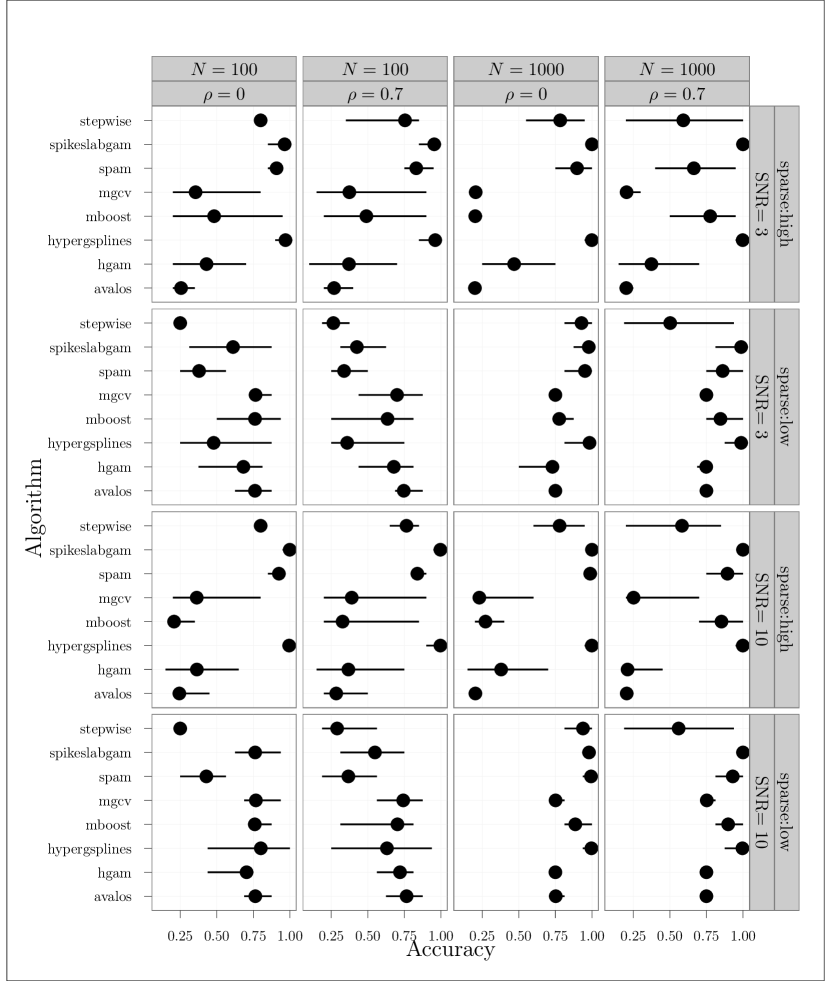
Figure 2: Proportion of correctly in- or excluded covariates for the different settings and algorithms. Rows for the different combinations of sparsity and signal-to-noise ratio, columns for the different combinations of number of observations $N$ and correlation $\rho$ of the covariates. Dot denotes mean accuracy, lines stretch from minimum to maximum accuracy observed over the 50 replications. Note that results for stepwise are not shown for correlated responses since it did not return reasonable predictions. Also note that hypergsplines did not return results for some data sets and only available fits are shown here.

Figure 3 shows computation times for the different algorithms and settings

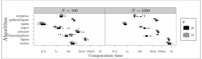
Figure 3: Computation times. Boxplots are color-coded for the dimensionality of the covariate vector. $p=20$ corresponds to the sparse setting with 4 no-zero and 16 zero effects and $p=16$ corresponds to the non-sparse setting with 12 non-zero and 4 zero effects. Horizontal axis on $\log_{10}$-scale. Note that results for stepwise do not include timings for correlated responses since it did not return sensible fits there. Also note that hypergsplines did not return results for some data sets and only timings for the available fits are shown here.

Most implementations were very stable, returning useful results for all 7200 model fits. Notable exceptions were stepwise, which failed to return reasonable fits for any replication of the settings with correlated covariates, and hypergsplines, which did not return predictions for 37 [47] of the 50 replicates for $N=100$, SNR$=3$ and low sparsity and correlation 0 [0.7] and also failed in 25 replications for $N=100$, SNR$=3$, low sparsity and correlation 0.7. Graphs and discussed results are based on all available results. Using only replicates for which hypergsplines also returned predictions would not change the results qualitatively.

Results for relative RMSE (c.f. Figure 1)):

• for small $N$, low SNR (4 panels on top left), spikeslabgam and hgam consistently beat the error of the oraclemgcv benchmark – hypergsplines does too, but only for the sparse setting.

• for small $N$, high SNR (4 panels on bottom left), spikeslabgam, hgam and hypergsplines consistently beat the error of the oraclemgcv benchmark. mboost and avalos also do well for the sparse setting.

• for larger $N$ (two rightmost columns), spikeslabgam, mgcv and, to a lesser extent, hypergsplines achieve performance very close to that of oraclemgcv. stepwise does too, but only for non-correlated responses. spam and mboost do (much) worse than oraclemgcv across the board for large $N$.

Results for selection accuracy (c.f. Figure 2)):

• with the notable exception of mboost in high $N$, high sparsity settings and stepwise, selection accuracy is robust against correlated covariates for all algorithms.

• for $N=1000$, spikeslabGAM, hypergsplines, and to a lesser extent spam as well have almost perfect accuracy across the board.

• for $N=100$, we see a clear split into algorithms that tend to fit very sparse models (spikeslabGAM, spam, hypergsplines) and consequently do well in the sparse settings and more liberal algorithms (mgcv, mboost, hgam) that do relatively better in the non-sparse settings. In the less noisy non-sparse settings, spikeslabGAM and hypergsplines also do well.

Computation times are displayed in Figure 3. The times of avalos and hgam scale very badly for larger data set size, while computation times for other methods that exhibit better or at least competitive selection and estimation performance (i.e., spikeslabGAM, hypergsplines, and, to a lesser extent, mboost) remain feasible. As hypergsplines first samples only the model indicators and then samples from a selection of models with strong posterior support to arrive at model-averaged effect estimates, it achieves a significant speed-up in the sparse case ($p=20$) where the models to be sampled in the second step are very small. All other methods are slower for $p=20$ than for $p=16$. Note that timings for spikeslabGAM, hypergsplines and mboost are (very) pessimistic since they do not make use of the parallelization features available for these 3 algorithms (parallel MCMC chains for spikeslabGAM, parallel computation via OpenMP for hypergsplines, parallel bootstrap iterations to determine the stopping iteration for mboost).

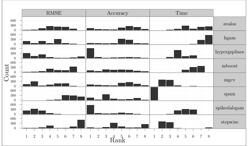
Figure 4: Rank distributions achieved by the 8 different algorithms for the AM simulation. Ties broken by assigning minimum rank to all involved.

Figure 4 shows the distribution of ranks achieved on each replicate of each setting by the 8 different algorithms in order to directly compare relative performance in terms of RMSE, selection accuracy and required computation time. spam and stepwise are fast, but not competitive in terms of estimation or selection. spikeslabgam and hypergsplines deliver the best estimation and selection performance, with slightly more best performances in shorter time for hypergsplines, but more stable results for spikeslabgam. hgam often delivers good estimates, but it is very slow. The best compromise in terms of accurate estimation and computation time seems to be offered by mgcv, but the selection accuracy is below average. Both mboost and avalos show intermediate results in all three performance dimensions we consider. Note that the threshold of $>10^{-5}$ effective degrees of freedom for inclusion of a term that we use for spam and mgcv is very low, leading to comparably less sparse models and more falsely included covariates than for most other methods, especially so for mgcv. In that sense, results for the selection accuracy of mgcv and, to a lesser extent, spam are somewhat pessimistic, especially in sparse settings.

4.2 Simulation study 2: Additive model with concurvity

To investigate the various methods’ robustness to concurvity, we use a similar data generating process as the one used in the previous Subsection:

• We define functions $f_{1}(x)$ to $f_{4}(x)$ as in the data generating process for the previous Subsection.

• We use $p=10$ or $p=20$ covariates: The first 4 are associated with functions $f_{1}$ to $f_{4}$, respectively, while the remainder are “noise” variables without contribution to the additive predictor.

• covariates $x$ are $\sim U[-2,2]$

• we distinguish 3 scenarios of concurvity:

  • in scenario 1, $x_{4}=c\cdot g(x_{3})+(1-c)\cdot u$, i.e., two covariates with real influence on the predictor are functionally related.

  • in scenario 2, $x_{5}=c\cdot g(x_{4})+(1-c)\cdot u$, i.e., a “noise” variable is a noisy version of a function of a covariate with direct influence.

  • in scenario 3, $x_{4}=c\cdot g(x_{5})+(1-c)\cdot u$, i.e., a covariate with direct influence is a noisy version of a “noise” variable.

  where $g(x)=2\Phi(x,\mu=-1,\sigma^{2}=0.16)+2\Phi(x,\mu=1,\sigma^{2}=0.09)-4\phi(x)-2$ with $\Phi(x,\mu,\sigma^{2})$ defined as the cdf of the respective Gaussian distribution, $\operatorname{i.i.d.}$ standard normal variates $u$, and the parameter $c$ controlling the amount of concurvity: $c=1$ for perfectly deterministic relationship, and $c=0$ for independence. In our simulation, $c=0,.2,.4,.6,.8,1$.
  

• we use signal-to-noise ratio SNR$=1,3$.

• we use $n=100$ observations for the training data set.

• we simulate 50 replications for each combination of the various settings.

Predictive MSE is evaluated on test data sets with 5000 observations. A similar simulation study setup has previously been used for comparing a different set of selection and estimation algorithms in Scheipl et al. [2012]. stepwise was omitted from this comparison due to its dismal performance for correlated covariates (see previous subsection). Note that mgcv did not return any fits for $p=20$ as it cannot be used to estimate models with more coefficients than observations.

Figure 5 shows relative predictive RMSE for $y$ for the 7 algorithms and the three scenarios under different concurvity, number of potential predictors $p$ and signal-to-noise ratio.

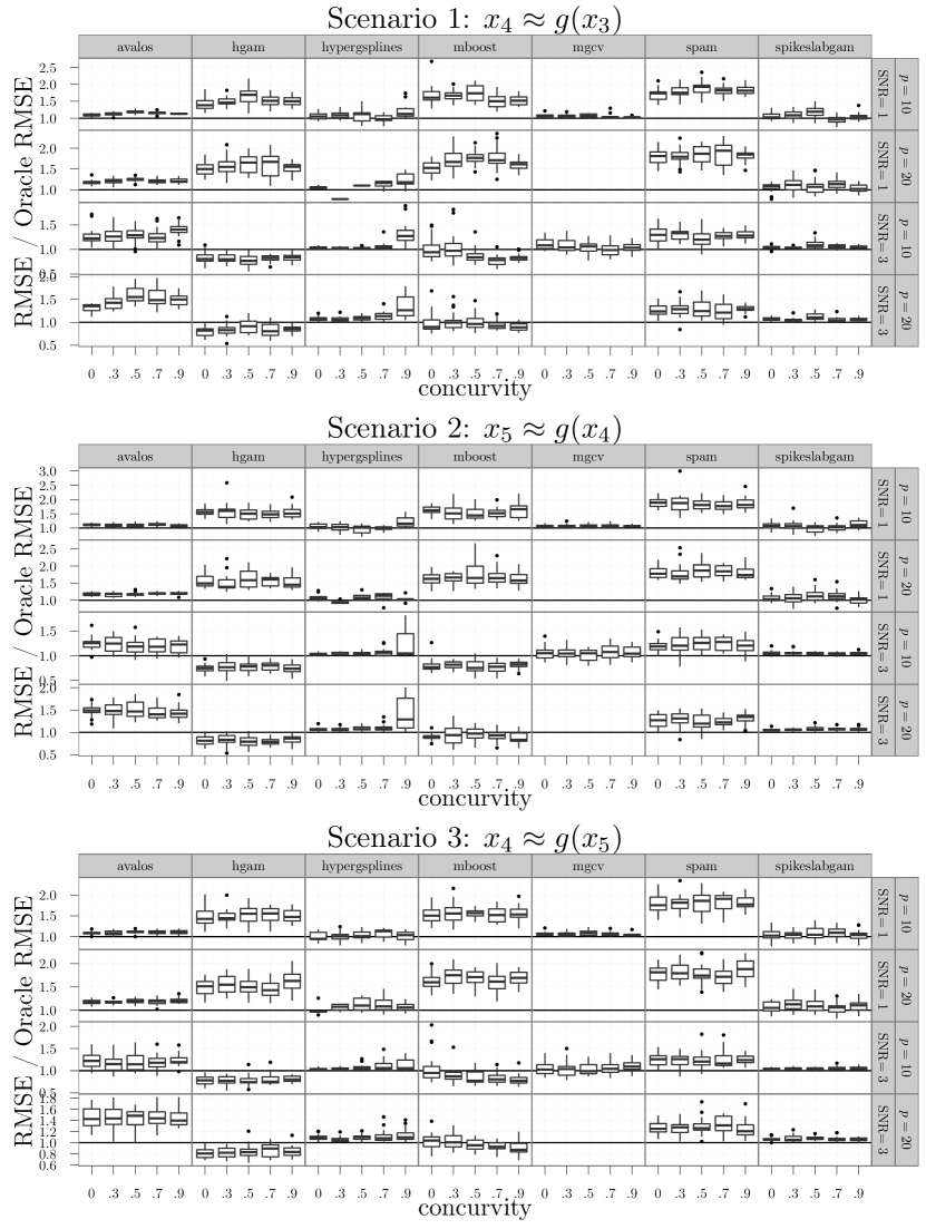
Figure 5: Boxplots of prediction RMSE divided by prediction RMSE of the “true” model fit by mgcv. Horizontal line denotes relative RMSE of 1, i.e. parity with the “oracle” model. Columns correspond to the different algorithms, rows correspond to the 4 combinations of number of potential predictors $p$ and signal to noise ratio. Results for mgcv for $p=20$ are missing as it cannot deal with models with more coefficients than observations.

Results for relative RMSE under concurvity (c.f. Figure 5):

• Overall estimation accuracy of $E(y)$ seems fairly robust against increasing concurvity and different number of noise terms for all the methods we consider here. Relevant increases in the relative error as concurvity increases are visible only for hypergsplines in Scenarios 1 and 2.

• hypergsplines, mgcv and spikeslabgam achieve performance almost equivalent to or better than the “true” model estimates across the board.

• mboost and hgam dominate the other methods and the “true” model estimates for higher signal-to-noise ratios (lower two lines in each figure), but are not competitive for more noisy data (upper two lines in each figure).

4.3 Benchmark study on binary response data

We investigated the performance of a subset of algorithms on four real data sets for binary classification taken from the UCI Machine Learning Repository [Frank and Asuncion, 2010]: the “Musk (Version 1)” (musk), “Liver Disorders” (liver), “Connectionist Bench (Sonar, Mines vs. Rocks)” (sonar) and “Pima Indian Diabetes” (pima) datasets. These datasets were picked since they do not contain any categorical predictors for which none of the algorithms except mboost and spikeslabgam can perform selection. Of the implementations described in the previous section, only hgam, hypergsplines, mboost, mgcv and spikeslabgam can deal with non-Gaussian data, so our comparison is limited to those five approaches.

Table 2 summarizes properties of the four datasets.

Name	$n$	$p$	$n/p$	Balance
liver	345	7	$49$	$1.4$
musk	467	167	$2.8$	$1.3$
sonar	208	61	$3.4$	$1.1$
pima	768	9	$85$	$1.9$

Table 2: Properties of the four benchmark datasets. $n$ denotes the number of observations, $p$ denotes the number of potential covariates, “Balance” is the ratio of the number of cases in the larger class divided by the number of cases in the smaller class, i.e., it is 1 if the data set has equal number of successes (ones) and failures (zeros).

Note that only musk, and, to a lesser extent, sonar, are truly high-dimensional variable selection problems and that only pima is somewhat unbalanced with a ratio of about 2:1 between cases in the bigger class and cases in the smaller class.

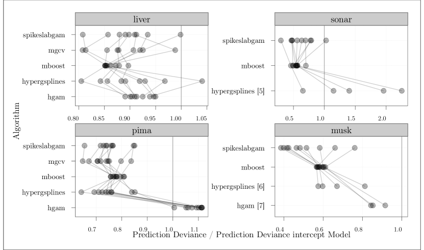
Figure 6: Dotplots of relative predictive deviance on the test data sets. Relative predictive deviance is defined as twice the negative log-likelihood evaluated on the test data sets divided by the predictive deviance of the intercept model on the training data, i.e., lower is better and values above 1 indicate predictions worse than those of a simple intercept model on average and indicate substantial overfitting. Results on the same test set connected by lines. Numbers in brackets after algorithm names indicate the number of times the algorithm failed to fit a model and/or return predictions. For the datasets in the right column, the full models have more coefficients than observations.

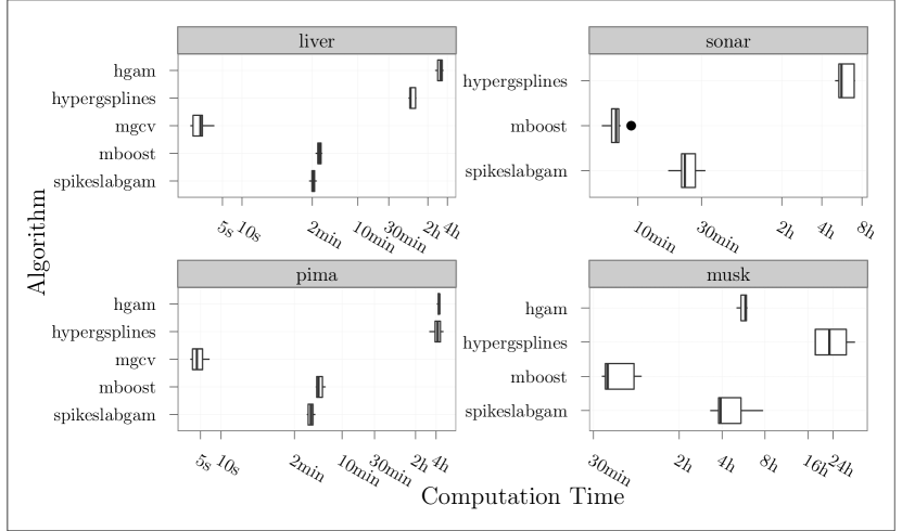
Figure 7: Boxplots of computation time for binary classification data sets in minutes. Time axis on binary log-scale.

For each of the four datasets, we generated ten bootstrap training data sets and evaluated predictive performance for the fitted additive logistic models in terms of minus twice the log likelihood (deviance) on the out-of-bag samples. To avoid extrapolation issues for the smooth terms, all training data sets contain those observations with the minimal and maximal values of the potential covariates for each data set. Figure 6 depicts the ratio between the predictive deviance of the fitted models and a simple logistic intercept model fitted on the training data, i.e., lower is better. Values above 1 indicate predictions worse than those of the simplest conceivable model on average and indicate substantial overfitting. Note that mgcv can not fit the musk and sonar datasets since the full model would have more coefficients than observations. hgam did not return any predictions for sonar due to numerical problems. For the remaining data sets, numbers in brackets after algorithm names indicate the number of times the algorithm failed to fit a model and/or return predictions. Results for the binary classification benchmark (c.f. Figures 6, 7) show that:

• mgcv and spikeslabgam have very similar predictive performances for the small data sets (liver, pima), but mgcv is orders of magnitude faster than all of the other algorithms.

• mboost’s performance is the most stable across replicates on each dataset and competitive to the best methods (mgcv and spikeslabgam). Its computation time is about the same as that of spikeslabgam for the small data sets and three to eight times faster for the high-dimensional problems.

• spikeslabgam performs consistently well on all four data sets, but its computation time is much larger than that of its closest competitor on the small data sets (mgcv) and its closest competitor on the large data sets (mboost).

• hgam’s performance is also fairly stable across replicates for the small data sets, but much less competitive. For the high-dimensional data sets, it becomes very unstable and does not return predictions at all for seven out of ten replicates for musk and no predictions at all for sonar.

• the performance for hypergsplines is similar but slightly worse than spikeslabgam for the smaller problems, but a lack of numerical stability of the implementation leads to a failure to return any predictions for five of the sonar test sets and six of the musk data sets. The remaining fits for the high-dimensional problems are not competitive, with relative predictive deviance values above 1 for the Sonar dataset indicating severe overfitting.

• computation times for hypergsplines and hgam are much larger than those of the other algorithms which yield better predictions in shorter time. The time difference is two orders of magnitude for the small datasets.

5 Conclusions

Currently, function selection is mainly concentrated on additive predictors of scalar Gaussian or exponential family responses. Extensions to other regression models for scalar responses, such as survival models, quantile regression and other beyond mean regression models would be desirable but are still sparse or completely lacking. A wide and open field for future research is variable and function selection in multivariate regression and latent variable models, where the association structure may also depend on covariates.

References

- Avalos et al. [2007] M. Avalos, Y. Grandvalet, and C. Ambroise. Parsimonious additive models. Computational Statistics and Data Analysis, 51:2851–2870, 2007.
- Belitz and Lang [2008] C. Belitz and S. Lang. Simultaneous selection of variables and smoothing parameters in structured additive regression models. Computational Statistics and Data Analysis, 53:61–81, 2008.
- Belitz et al. [2012] C. Belitz, A. Brezger, T. Kneib, S. Lang, and N. Umlauf. BayesX - Software for Bayesian inference in structured additive regression models, 2012. URL http://www.stat.uni-muenchen.de/~bayesx. Version 2.1.
- Bühlmann and Hothorn [2007] P. Bühlmann and T. Hothorn. Boosting algorithms: Regularization, prediction and model fitting. Statistical Science, 22:477–505, 2007.
- Bühlmann and Yu [2003] P. Bühlmann and B. Yu. Boosting with the loss: Regression and Classification. Journal of the American Statistical Association, 98:324–339, 2003.
- Cottet et al. [2008] R. Cottet, R.J. Kohn, and D.J. Nott. Variable Selection and Model Averaging in Semiparametric Overdispersed Generalized Linear Models. Journal of the American Statistical Association, 103:661–671, 2008.
- Eaton et al. [2008] J. W. Eaton, D. Bateman, and S. Hauberg. GNU Octave Manual Version 3. Network Theory Limited, 2008.
- Eilers and Marx [1996] P. H. C. Eilers and B. D. Marx. Flexible smoothing using B-splines and penalized likelihood. Statistical Science, 11:89–121, 1996.
- Eugster et al. [2010] M.A. Eugster, T. Hothorn(Authors), H. Frick, I. Kondofersky, O. S. Kuehnle, C. Lindenlaub, G. Pfundstein, M. Speidel, M. Spindler, A. Straub, F. Wickler, and K. Zink (Contributors). hgam: High-Dimensional Additive Modelling, 2010. R package version 0.1-0.
- Fahrmeir and Kneib [2011] L. Fahrmeir and T. Kneib. Bayesian smoothing and regression for longitudinal, spatial and event history data. Oxford Statistical Science Series 36, Oxford, 2011.
- Fahrmeir et al. [2010] L. Fahrmeir, T. Kneib, and S. Konrath. Bayesian regularization in structured additive regression: A unifying perspective on shrinkage, smoothing and predictor selection. Statistics and Computing, 20:203–219, 2010.
- Fan and Li [2001] J. Fan and R. Li. Variable selection via nonconcave penalized likelihood and its oracle properties. Journal of the American Statistical Association, 96:1348–1360, 2001.
- Frank and Asuncion [2010] A. Frank and A. Asuncion. UCI machine learning repository, 2010. URL http://archive.ics.uci.edu/ml.
- George and McCulloch [1993] E.I. George and R.E. McCulloch. Variable selection via Gibbs sampling. Journal of the American Statistical Association, 88:881–889, 1993.
- George and McCulloch [1997] E.I. George and R.E. McCulloch. Approaches for Bayesian Variable Selection. Statistica Sinica, 7:339–374, 1997.
- Griffin and Brown [2005] J.E. Griffin and P.J. Brown. Alternative prior distributions for variable selection with very many more variables than observations. Technical Report UKC/IMS/05/08, IMS, University of Kent, 2005.
- Gu [2002] C. Gu. Smoothing Spline ANOVA Models. Springer-Verlag, 2002.
- Hothorn et al. [2012] T. Hothorn, P. Bühlmann, T. Kneib, M. Schmid, and B. Hofner. mboost: Model-Based Boosting, 2012. R package version 2.1-1.
- Huang et al. [2010] J. Huang, J.L. Horowitz, and F. Wei. Variable selection in nonparametric additive models. Annals of Statistics, 38:2282–2313, 2010.
- Ishwaran and Rao [2005] H. Ishwaran and J.S. Rao. Spike and slab variable selection: frequentist and Bayesian strategies. Annals of Statistics, 33(2):730–773, 2005.
- Kneib et al. [2009] T. Kneib, T. Hothorn, and G. Tutz. Variable selection and model choice in geoadditive regression models. Biometrics, 65:626–634, 2009.
- Kneib et al. [2011] T. Kneib, S. Konrath, and L. Fahrmeir. High-dimensional structured additive regression models: Bayesian regularisation, smoothing and predictive performance. Applied Statistics, 60:51–70, 2011.
- Konrath et al. [2012] S. Konrath, L. Fahrmeir, and T. Kneib. Bayesian smoothing, shrinkage and variable selection in hazard regression. 2012.
- Leng and Zhang [2006] C. Leng and H.H. Zhang. Model selection in nonparametric hazard regression. Nonparametric Statistics, 18:417–429, 2006.
- Lin and Zhang [2006] Y. Lin and H.H. Zhang. Component selection and smoothing in multivariate nonparametric regression. Annals of Statistics, 34:2272–2297, 2006.
- Marra and Wood [2011] G. Marra and S. Wood. Practical variable selection for generalized additive models. Computational Statistics and Data Analysis, 55:2372–2387, 2011.
- MATLAB [2010] MATLAB. MATLAB version 7.10.0 (R2010a). The MathWorks Inc., Natick, Massachusetts, 2010.
- Meier [2009] L. Meier. grplasso: Fitting user specified models with Group Lasso penalty, 2009. R package version 0.4-2.
- Meier et al. [2008] L. Meier, S. van de Geer, and P. Bühlmann. The group Lasso for logistic regression. Journal of the Royal Statistical Society Series B, 70:53–71, 2008.
- Meier et al. [2009] L. Meier, S. van der Geer, and P. Bühlmann. High-dimensional additive modeling. Annals of Statistics, 37:3779–3821, 2009.
- O’Hara and Sillanpää [2009] R.B. O’Hara and M.J. Sillanpää. A Review of Bayesian Variable Selection Methods: What, How, and Which? Bayesian Analysis, 4:85–118, 2009.
- Panagiotelis and Smith [2008] A. Panagiotelis and M. Smith. Bayesian identification, selection and estimation of semiparametric functions in high-dimensional additive models. Journal of Econometrics, 143:291–316, 2008.
- Park and Casella [2008] T. Park and G. Casella. The Bayesian lasso. Journal of the American Statistical Association, 103:681–686, 2008.
- Polson and Scott [2012] N. G. Polson and J. G. Scott. Local shrinkage rules, Lévy processes and regularized regression. Journal of the Royal Statistical Society Series B, 74(2):287–311, 2012.
- R Development Core Team [2011] R Development Core Team. R: A Language and Environment for Statistical Computing. R Foundation for Statistical Computing, Vienna, Austria, 2011. URL http://www.R-project.org/.