Environmental Time Series Interpolation Based on Spartan Random Processes

Abstract

In many environmental applications, time series are either incomplete or irregularly spaced. We investigate the application of the Spartan random process to missing data prediction. We employ a novel modified method of moments (MMoM) for parameter inference. The CPU time of MMoM is shown to be much faster than that of maximum likelihood estimation and almost independent of the data size. We formulate an explicit Spartan interpolator for estimating missing data. The model validation is performed on both synthetic data and real time series of atmospheric aerosol concentrations. The prediction performance is shown to be comparable with that attained by the best linear unbiased (Kolmogorov-Wiener) predictor at reduced computational cost.

1 Introduction

Time series have wide-ranging applications in environmental monitoring, such as air and water quality control. The series carry information about temporal autocorrelations (henceforth, correlations) in variables such as atmospheric pollutant concentrations, particulate matter, indicators of water clarity, salinity etc. Knowledge of the correlation structure enables the prediction of time-series, estimating the prediction uncertainty, and developing stochastic simulations that reconstruct (at least partially) the process of interest. In many applications, observations are irregularly spaced (due to difficulties and cost of data acquisition), and they include fully missing (due to measurement interruptions) or censored (lying below the equipment detection threshold) data. These gaps in the series prevent the use of standard analytical techniques that assume regular sampling. Recently, the European Union introduced a novel concept in environmental legislation, in an effort to establish common data quality objectives for air pollution (Ballesta,, 2005). Hence, there is a need to harmonize data obtained by means of different measurement techniques and sampling conditions. Difficulties in quantifying uncertainty, due to incomplete time coverage, led to simplistic approaches that assume a random distribution of the missing data. The associated uncertainty is then reduced to a simple function of the percentage of the missing data. However, neglecting the frequency distribution and temporal correlations of the missing data can strongly affect the estimates. Furthermore, the data may be sampled at different temporal scales. By predicting time series at unmeasured instants, it is possible to fill in the missing values or to down-scale (refine) existing measurements.

Several recent papers evaluate methods of time series prediction for environmental applications. In (Houseman,, 2005), a first-order autoregressive model was applied to irregularly spaced water clarity data. Multivariate models have been applied to the time series of pollutant concentrations in the Arctic, using the multiple imputation approach (Hopke et al.,, 2001). Time series of aerosol particle number concentrations were modeled on the basis of traffic-related air pollution and meteorological variables (Paatero et al.,, 2005). In (Junninen et al.,, 2004), the authors evaluate and compare various univariate and multivariate methods for missing data imputation in air quality data sets. Generally, the simple univariate models that either utilize only local information or make linearity assumptions, are fast but their scope is limited. Multivariate models provide higher accuracy and reliability at increased computational cost. In the current study, we present a novel linear predictor, which is based on the use of “pseudo-energy” functionals inspired from statistical physics. We apply this Spartan predictor in conjunction with computationally efficient parameter inference method. We show that the results obtained with the Spartan predictor are comparable with those obtained by the best linear unbiased estimator. However, the former is superior in terms of computational speed.

For Gaussian time series, the temporal structure is determined from the autocovariance (henceforth, covariance) matrix, which is estimated from the data. In the case of non-uniform sampling steps, the structure function (variogram) is typically estimated instead of the covariance for practical reasons. However, temporal correlations are also present (albeit on different physical scales) in models of statistical physics, e.g., in the Ising model and spin glass models. In these models, correlations are imposed by means of physical interactions embodied in the energy functional and thus do not need to be calculated from the data. Recently, the method of Spartan Spatial Random Fields (SSRF) (Hristopulos,, 2003; Hristopulos and Elogne,, 2007) was proposed as a general framework for geostatistical applications. SSRFs are parametrically flexible, do not rely on variogram estimation to determine the spatial structure, and allow incorporating physical constraints in the joint probability density function. In the present study, we define in the same spirit the Spartan Random Processes (SRP) and apply them to time series prediction.

The rest of the paper is organized as follows. Spartan random processes are introduced in Section 2. In Section 3, we discuss parameter inference using maximum likelihood estimation and the modified method of moments. In Section 4 we present the Spartan interpolator and compare it to the Kolmogorov Wiener predictor (simple kriging). In Sections 5 and 6, we compare the model inference and data prediction methods using both synthetic data as well as real time series of aerosol concentration. Finally, we summarize and present our conclusions in Section 7.

2 Spartan Random Processes

Herein we assume a Gaussian, second-order stationary (Yaglom,, 1987), detrended time series, $X_{\lambda}(t);$ $\lambda$ is an intrinsic time scale related to temporal resolution. The pdf can be expressed in terms of an energy functional ${H[X_{\lambda}({t})]}$, according to the familiar from statistical physics expression of Gibbs pdf’s:

$$f_{\rm x}[X_{\lambda}]=Z^{-1}\,e^{-H[X_{\lambda}(t)]},$$ (1)

where the partition function $Z$ is the normalization factor. In the classical geostatistical framework the energy functional corresponds to:

$$H[X_{\lambda}]=\frac{1}{2}\sum_{i=1}^{N}\sum_{j=1}^{N}X_{\lambda}(t_{i})\,[G_{\rm x}]^{-1}_{i,j}X_{\lambda}(t_{j}),$$ (2)

where $[G_{\rm x}]^{-1}_{i,j}$ is the inverse of the covariance matrix (also known as the precision matrix), and $N$ is the number of the data points.

In analogy with Spartan spatial random fields (Hristopulos,, 2003), we define the fluctuation-gradient-curvature (FGC) Spartan random process that involves four parameters with a well defined physical meaning: the scale coefficient $\eta_{0}$, the shape coefficient $\eta_{1}$, the characteristic time $\xi$, and the cutoff circular frequency $k_{c}\propto\lambda^{-1}$. A kernel function is used to implement the cutoff. Below we use a boxcar kernel with sharp spectral cutoff at $k_{c}.$ If time is considered as a continuous variable, the FGC Spartan pdf is determined from the following energy functional:

$$H_{\rm fgc}[X_{\lambda};\bm{\theta}]=\frac{1}{{2\eta_{0}\xi}}\int_{-\infty}^{\infty}{dt}\,\left\{\left[{X_{\lambda}(t)}\right]^{2}+\eta_{1}\,\xi^{2}[{\dot{X}_{\lambda}(t)}]^{2}+\xi^{4}[{\ddot{X}_{\lambda}(t)}]^{2}\right\},$$ (3)

where $\bm{\theta}=(\eta_{0},\eta_{1},\xi,k_{c})$ and the dots denote the first and second order time derivatives. The covariance spectral density is then given by the following expression

$$\tilde{G}_{\rm x}(k;\bm{\theta})=\frac{h_{\lambda}(k)\,\eta_{0}\,\xi}{1+\eta_{1}\,(k\xi)^{2}+(k\xi)^{4}},$$ (4)

where $h_{\lambda}(k)=1,$ if $k\leq k_{c}$ and $h_{\lambda}(k)=0$ otherwise. The covariance function is then obtained from the inverse Fourier transform, given by the following integral:

$$G_{\rm x}(\tau;\bm{\theta})={\int}_{-\infty}^{\infty}\frac{dk}{2\pi}\,\tilde{G}_{\rm x}(k;\bm{\theta})\,e^{\jmath k\tau}.$$ (5)

For a discrete time series, sampled at the times $t_{n}=n\alpha$, $n=1,\ldots,N$, $\alpha>0$, the derivatives are approximated by finite forward differences and the energy functional takes the following form:

$$H_{\rm fgc}\left[X_{\lambda};{\bm{\theta}}\right]=\frac{1}{2\eta_{0}\xi}\sum\limits_{n=1}^{N}\left\{S_{0}(t_{n})+\eta_{1}\,\xi^{2}S_{1}(t_{n})+\xi^{4}S_{2}(t_{n})\right\},$$ (6)

where

$$S_{0}(t_{n})=X_{\lambda}(t_{n})^{2},$$

$$S_{1}(t_{n})=\left[\frac{X_{\lambda}(t_{n}+\alpha)-X_{\lambda}(t_{n})}{\alpha}\right]^{2},$$

$$S_{2}(t_{n})=\frac{\left[X_{\lambda}(t_{n}+\alpha)+X_{\lambda}(t_{n}-\alpha)-2X_{\lambda}(t_{n})\right]^{2}}{\alpha^{4}}.$$

2.1 The Precision Matrix

In Eq. (2), the values of the process are coupled even at distant times through the precision matrix. In contrast, in Eq. (6) only values between neighboring times are coupled. The energy functional is then expressed as follows:

$$H_{{\rm{fgc}}}\left[X_{\lambda};\bm{\theta}\right]=\frac{1}{2}X_{\lambda}(t_{i})J_{\rm x}(t_{i},t_{j};\bm{\theta})X_{\lambda}(t_{j}),$$ (7)

where $J_{\rm x}(t_{i},t_{j};\bm{\theta})$ is the precision matrix. Based on Eq. (6), the precision matrix can be expressed in closed form as follows:

$$J_{{\rm{x}}}(t_{i},t_{j};\bm{\theta})=\frac{1}{\eta_{0}\xi}\Bigg{\{}J_{0}(t_{i},t_{j})+\eta_{1}\frac{\xi^{2}}{\alpha^{2}}J_{1}(t_{i},t_{j})+\frac{\xi^{4}}{\alpha^{4}}J_{2}(t_{i},t_{j})\Bigg{\}},$$ (8)

where $J_{0}(t_{i},t_{j})=\delta_{i,j}$ is the identity matrix, $J_{1}(t_{i},t_{j})$ is the gradient precision sub-matrix,

$$J_{1}(t_{i},t_{j})=\left(\begin{array}[]{ccccc}1&-1&0&\cdots&0\\ -1&2&-1&\cdots&0\\ &\ddots&\ddots&\ddots&\\ 0&\cdots&-1&2&-1\\ 0&\cdots&0&-1&1\\ \end{array}\right),$$ (9)

and $J_{2}(t_{i},t_{j})$ is the curvature precision sub-matrix

$$J_{2}(t_{i},t_{j})=\left(\begin{array}[]{cccccc}1&-2&1&0&\cdots&0\\ -2&5&-4&1&\cdots&0\\ 1&-4&6&-4&1&0\\ &\ddots&\ddots&\ddots&\ddots&\\ 0&\cdots&1&-4&5&-2\\ 0&\cdots&0&1&-2&1\\ \end{array}\right).$$ (10)

In the discrete representation, given by Eqs. (7)-(10), the Spartan random process is equivalent to a Markov random process, the only difference from the latter being the nonlinear dependence on the coefficients. However, in contrast with Markov processes, the Spartan random process can be generalized to non-uniform sampling patterns as shown in (Elogne et al.,, 2008).

3 Parameter Inference

Let $T_{\rm s}=\{t_{1},...,t_{N}\}$ be a set of sampling times and ${\bf X}^{*}(T_{\rm s})=\{X^{*}_{1},...,X^{*}_{N}\}$ the vector of sample measurements. Let $L(\bm{\theta}|{\bf X}^{*})$ denote the likelihood of the parameter vector $\bm{\theta}$ given the data. Let us also define the reduced parameter set $\bm{\theta^{\prime}}=(\eta_{1},\xi,k_{c})$ and the scaled precision matrix $J^{\prime}_{\rm x}(\bm{\theta^{\prime}})=\eta_{0}\,J_{\rm x}(\bm{\theta}).$ Let the sample estimate of the energy functional be $\hat{H}_{\rm{fgc}}\left[X_{\lambda};\bm{\theta}\right]$. The scaled energy functional is defined by $\hat{H^{\prime}}_{\rm{fgc}}\left[X_{\lambda};\bm{\theta^{\prime}}\right]=\eta_{0}\,\hat{H}_{\rm{fgc}}\left[X_{\lambda};\bm{\theta}\right]$.

For a complete (with no missing data) series $\hat{H}_{\rm{fgc}}\left[X_{\lambda};\bm{\theta}\right]$ is given from equation (7) by replacing $X_{\lambda}(t_{i})$ with the data $X^{*}(t_{i}).$

In the case of series with missing data it is preferable to use the definition

$$\hat{H}_{\rm fgc}\left[X_{\lambda};{\bm{\theta}}\right]=\frac{N}{2\eta_{0}\xi}\left\{\overline{S_{0}(t)}+\eta_{1}\,\xi^{2}\overline{S_{1}(t)}+\xi^{4}\overline{S_{2}(t)}\right\},$$ (11)

where $\overline{S_{q}}$ are sample estimates of the respective quantities $S_{q},\,q=0,1,2$, evaluated over all the time instants present in the series. The gaps do not influence the estimation of $\overline{S_{0}}$, which is performed over all the sample points. In the case of $\overline{S_{1}},$ the average involves all compact clusters of data that include at least two nearest neighbors. Similarly, in the case of $\overline{S_{2}},$ the average involves all compact clusters of data that include at least three nearest neighbors.

3.1 Maximum Likelihood Estimation

The maximum likelihood estimates (MLE) are obtained by minimizing numerically the negative log-likelihood (NLL), e.g. (Stein,, 1999, pp. 169-175), which requires the evaluation and inversion of the covariance matrix. The numerical operations are computationally intensive, especially for large sample sizes. As we show below, the Spartan random process has a significant advantage in terms of computational speed. The NLL becomes:

$$-\log L(\bm{\theta}|{\bf X}^{*})=\frac{\hat{H^{\prime}}_{\rm{fgc}}\left[X_{\lambda};\bm{\theta^{\prime}}\right]}{\eta_{0}}+\frac{N}{2}\log(\eta_{0})+\frac{N}{2}\log(2\pi)-\frac{1}{2}\log|J^{\prime}_{\rm x}(\bm{\theta^{\prime}})|.$$ (12)

The estimate $\hat{\eta}_{0}$ follows from requiring the derivative of $\log L(\bm{\theta}|{\bf X}^{*})$ with respect to $\eta_{0}$ to vanish, leading to,

$$\hat{\eta}_{0}=\frac{2\hat{H^{\prime}}_{\rm{fgc}}\left[X_{\lambda};\bm{\theta^{\prime}}\right]}{N},$$ (13)

and by replacing $\eta_{0}$ with $\hat{\eta}_{0}$ in equation (12), the NLL is given in terms of the scaled variables $\hat{H^{\prime}}_{\rm{fgc}}\left[X_{\lambda};\bm{\theta^{\prime}}\right]$ and $J^{\prime}_{\rm x}(\bm{\theta^{\prime}})$ as follows:

$$-\log L(\bm{\theta}|{\bf X}^{*})=\frac{N}{2}\log\bigg{(}{2\hat{H^{\prime}}_{\rm{fgc}}\left[X_{\lambda};\bm{\theta^{\prime}}\right]/N}\bigg{)}-\frac{1}{2}\log|J^{\prime}_{\rm x}(\bm{\theta^{\prime}})|+C_{N}.$$ (14)

The constant $C_{N}=\frac{N}{2}[\log(2\pi)+1]$ is independent of $\bm{\theta^{\prime}}$ and can be dropped from the minimization. The NLL is minimized using a numerical optimization method. In the case of the Spartan random process, the computational efficiency is gained by the fact that $\hat{H^{\prime}}_{\rm{fgc}}\left[X_{\lambda};\bm{\theta^{\prime}}\right]$ is estimated without the inversion of a full covariance matrix. Moreover, based on equations (9) and (10), $J^{\prime}_{\rm x}(\bm{\theta^{\prime}})$ is a pentadiagonal symmetric matrix, so that fast and accurate approximations can be used for the evaluation of its determinant (Reusken,, 2002).

3.2 Modified Method of Moments

The modified method of moments (MMoM) is based on fitting stochastic constraints with their sample counterparts. The constraints are based on short-range correlations and are motivated from the terms $S_{m}(t_{n}),\ m=0,1,2$, in the energy functional (6). The stochastic constraints are expressed as follows:

$$E[S_{0}]=G_{\rm x}(0),$$ (15)

$$E[S_{1}]=\frac{2}{\alpha^{2}}\left[G_{\rm x}(0)-G_{\rm x}(\alpha)\right],$$ (16)

$$E[S_{2}]=\frac{2}{\alpha^{4}}\left[3G_{\rm x}(0)+G_{\rm x}(2\alpha)-4G_{\rm x}(\alpha)\right].$$ (17)

The stochastic constrains are functions of ${\bm{\theta}}$ obtained from spectral integrals (Hristopulos,, 2003). Herein we focus on time series with well defined temporal resolution and correlation times that exceed this resolution. Then, we can assume an infinite band limit ($k_{c}\rightarrow\infty$) and suppress the subscript $\lambda$. The respective Spartan covariance function has been evaluated in Hristopulos and Elogne, (2007), and it is given by the following:

$$G_{\rm x}(t)=\left\{\begin{array}[]{ll}\eta_{0}e^{-h\beta_{2}}\bigg{[}\frac{\cos(h\beta_{1})}{4\beta_{2}}+\frac{\sin(h\beta_{1})}{4\beta_{1}}\bigg{]},&{\rm{for}}\ |\eta_{1}|<2,\\ \eta_{0}\frac{(1+h)}{4e^{h}},&{\rm{for}}\ \eta_{1}=2,\\ \eta_{0}\frac{1}{\Delta}\bigg{[}\frac{e^{-h\omega_{1}}}{2\omega_{1}}-\frac{e^{-h\omega_{2}}}{2\omega_{2}}\bigg{]},&{\rm{for}}\ \eta_{1}>2,\end{array}\right.$$ (18)

where $h\equiv|\tau|/\xi$, $\beta_{1,2}=(|2\pm\eta_{1}|)^{1/2}/2$, $\omega_{1,2}=(|\eta_{1}\pm\Delta|/2)^{1/2}$, and $\Delta=|\eta_{1}^{2}-4|^{1/2}$. Hence, the stochastic constraints given by Eqs. (15-17) can be expressed analytically in terms of the covariance function. The optimal values of the model parameters are estimated by minimizing the following objective functional (Hristopulos,, 2003)

$$\Phi_{s}[X(t)]=\Bigg{|}1-\sqrt{\frac{\overline{S_{1}}}{\overline{S_{0}}}\frac{E[S_{0}]}{E[S_{1}]}}\Bigg{|}^{2}+\Bigg{|}1-\sqrt{\frac{\overline{S_{2}}}{\overline{S_{1}}}\frac{E[S_{1}]}{E[S_{2}]}}\Bigg{|}^{2}$$ (19)

The application of this distance metric (DM) is based on the following assumptions: First, the sample averages $\overline{S_{m}}$, $m=0,1,2$ are accurate and precise estimators of the stochastic expectations $E^{\prime}[S_{m}]$ of the underlying random process (where $E^{\prime}[.]$ denotes the expectation with respect to the unknown probability density). This assumes that ergodic conditions are satisfied, e.g. (Adler,, 1981). Second, the stochastic expectations $E[S_{m}]$ of the Gibbs random process should approximate the expectations $E^{\prime}[S_{m}]$ of the underlying process.

4 Prediction of Missing Data (Temporal Interpolation)

Let us assume that there are points where data are missing in the sampling set $T_{\rm s}.$ The missing points are included in the prediction set, $T_{\rm p}=\{z_{1},...,z_{P}\}$, which is assumed to be disjoint from $T_{\rm s}$. We denote by $\hat{\bf X}(T_{\rm p})$ the vector of estimates (temporal predictions). Finally, let $T=T_{\rm s}\cup T_{\rm p}$ and ${\bf X}(T)=\hat{\bf X}(T_{\rm p})\circ{\bf X}^{*}(T_{\rm s})$ be the joint vector of measurements and prediction points.

Using the Kolmogorov-Wiener theory (Kitanidis,, 1997; Wackernagel,, 2003), the single-point prediction at the point $z_{p},$ $\hat{X}(z_{p}),$ is given as a linear superposition of the data values. The coefficients of the superposition are selected so as to ensure zero bias and minimize the mean square error of the prediction, leading to the following Kolmogorov-Wiener prediction (KWP) equation:

$$\hat{X}(z_{p})=\left[{\bf G}^{-1}({\bm{\theta}};T_{\rm s},T_{\rm s})\,{\bf G}({\bm{\theta}};T_{\rm s},z_{p})\right]^{\rm tr}\,{\bf X}^{*}(T_{\rm s}),\ \ \ p=1,...,P.$$ (20)

In the above, ${\bf G}({\bm{\theta}};T_{\rm s},T_{\rm s})$ is the $N\times N$ data covariance matrix, ${\bf G}^{-1}$ is its inverse, ${\bf G}({\bm{\theta}};T_{\rm s},z_{p})$ is the $N\times 1$ covariance matrix between the estimated point and the data, and ${\bf A}^{\rm tr}$ denotes the transpose of the matrix ${\bf A}.$

The Spartan family of covariance functions, Eq. (18), can be used in KWP algorithms to provide new types of spatial dependence. Within the SRP framework it is also possible to define a new type of linear predictor, which allows multiple-point prediction to be performed simultaneously over all points in $T_{\rm p}$.

4.1 The Spartan predictor

The Spartan predictor (SP) defined below, is based on the FGC model. It relies on maximizing the conditional probability density, $f_{\rm x}[\hat{\bf X}(T_{\rm p})|{\bf X}^{*}(T_{\rm s})]$. Considering the definition $f_{\rm x}[\hat{\bf X}(T_{\rm p})|{\bf X}^{*}(T_{\rm s})]=f_{\rm x}[\hat{\bf X}(T_{\rm p})]/f_{\rm x}[{\bf X}^{*}(T_{\rm s})]$, the problem reduces to maximizing $f_{\rm x}[{\bf X}(T)]$. The latter involves the energy functional over the combined set of sampling and prediction points, i.e.,

$$\hat{H}_{\rm fgc}\left[{\bf X}(T);\bm{\theta}\right]=\frac{1}{2}{\bf X}^{\rm tr}(T)\,{\bf J}_{\rm x}(\bm{\theta})\,{\bf X}(T).$$ (21)

Maximizing the conditional probability with respect to the prediction values leads to the following linear system of $P$ equations

$$\frac{\partial\hat{H}_{fgc}[{\bf X}(T);\bm{\theta}]}{\partial X(z_{p})}\Bigg{|}_{\hat{X}(z_{p})}=0,\ \ \ p=1,\ldots,P.$$ (22)

The predictions do not depend on $\eta_{0}$, since the latter is an overall scaling factor for ${\bf J}_{\rm x}(\bm{\theta})$. If there are no interactions between the prediction points, i.e. $J_{\rm x}({\bm{\theta}};z_{i},z_{j})=0$, $i,j=1,...,P$, the linear predictor is expressed explicitly by

$$\hat{X}(z_{p})=-\sum_{t_{l}\in V(z_{p})}{\frac{J_{\rm x}({\bm{\theta}};t_{l},z_{p})}{J_{\rm x}({\bm{\theta}};z_{p},z_{p})}\,X^{*}(t_{l})},\ \ \ p=1,...,P,$$ (23)

where $V(z_{p})$ is the interaction neighborhood of $z_{p}$, i.e., the set of the points in $t_{l}\in T_{\rm s}$ that interact with $z_{p}$. In the case of the FGC functional the interaction neighborhood spreads up to the second-nearest neighbor.

The Spartan predictor is linear and unbiased. Unlike the KWP, it does not require computationally expensive calculations of the covariance matrix. Specifying an arbitrary search neighborhood for each prediction point is not necessary, since the SP uses only the data in the immediate interaction neighborhood. In KWP the estimation is performed sequentially point-by-point by solving a linear system of equations. In contrast, SP is a multi-point estimator and it can be formulated explicitly only if the interaction neighborhoods of the estimation points are disjoint. The numerical complexity of multipoint SP estimation is $O(P^{3})$, while the numerical complexity of KWP is $O(P\,M^{3})$, where $M$ is average number of points inside the local search neighborhood of the estimation points. In some trivial cases (Fig. 1), the equivalence between the FGC SP and KWP can be shown analytically, using symmetry of the precision and covariance matrices of the regularly spaced data. For longer time series, the analytical comparison becomes cumbersome and hence, we resort to comparison by numerical calculations. In a general case, however, we cannot expect equivalence of the two methods, since SP only considers the data from the short-range interaction neighborhood while KWP considers all the data available (or those from the search neighborhood, generally different from the SP interaction neighborhood). Nevertheless, in the multipoint Spartan prediction, the local information propagates through the system via the interacting prediction points, .i.e, system of coupled equations (22), influencing predictions at distant locations and, hence, its performance compared to KWP is a priori not obvious.

Figure 1: Some trivial time series, consisting of only 3 points, for which equivalence between SP and KWP can be shown analytically. The circles denote the known data and the crosses the prediction points.

5 Case Study I: Simulated Data

All the computations were performed in the Matlab$\circledR$ environment, on a desktop computer with Pentium 4 CPU at 3 GHz and 1 GB of RAM. We evaluate the performance of the MLE and the MMoM methods for parameter inference. We also compare the performance of the SP and KWP missing data estimators. First, we use control time series of sizes $N=100,200,300,500,1000$ based on the following covariance functions: (i) Gaussian $G_{\rm x;G}({\tau})=\sigma^{2}{\rm{exp}}(-h^{2}),$ (ii) exponential $G_{\rm x;E}({\tau})=\sigma^{2}{\rm{exp}}(-h),$ (iii) spherical $G_{\rm x;S}({\tau})=\sigma^{2}(1-1.5h+0.5h^{3})$ for $h\leq 1$ and $G_{\rm x;S}({\tau})=0$ for $h>1,$ and (iv) Whittle-Matérn $G_{\rm x;M}({\tau})=\sigma^{2}\frac{{2}^{1-\nu}}{\Gamma(\nu)}(\kappa\tau)^{\nu}K_{\nu}(\kappa\tau).$ In the above, $\sigma^{2}$ represents the variance, $b$ the correlation time, $h=|\tau|/b,$ the normalized time lag, $\nu$ the smoothness parameter, $\kappa$ the inverse length, and $K_{\nu}$ the modified Bessel function of index $\nu$. The samples are generated using the multivariate normal simulation method (Johnson,, 2004). The covariance parameters are: For the Gaussian $(\sigma,b)=(10,3)$, for the exponential and the spherical $(\sigma,b)=(10,5)$, and for the Whittle-Matérn: $(\sigma,\kappa,\nu)=(10,1,3.5)$. For each covariance model and size $N$, 100 time series ${\rm X}^{*}_{i}$ ($i=1,...,100$) are generated in order to calculate optimization and computer time statistics.

5.1 Results: Parameter Inference

The optimization employs the Nelder-Mead simplex search algorithm (Press et al.,, 1992) for both the MLE and the MMoM cases. This algorithm is fast, because it does not require the computation of a Jacobian matrix. The optimization is terminated when both the model parameters and the objective function (NLL for the MLE or DM for the MMoM) change between consecutive steps less than the specified tolerance, $\epsilon=10^{-6}$. The initial guesses for the Spartan parameters are $\xi^{(0)}_{i}=\alpha=1$, $\eta_{1}^{(0)}=-1$ (for the MLE different initial guesses $\eta_{1}^{(0)}$ are in order due to multimodality).

In Table 1, we compare the MLE and MMoM parameter inference methods, using time series with Gaussian correlations. The mean values of the estimated Spartan parameters, $\langle\eta_{0}^{*}\rangle$, $\langle\eta_{1}^{*}\rangle$ and $\langle\xi^{*}\rangle$ are listed, as well as their standard deviations $\hat{S}_{\eta_{0}^{*}}$, $\hat{S}_{\eta_{1}^{*}}$ and $\hat{S}_{\xi^{*}}$. The number of the optimization iterations $\langle N_{it}\rangle$, the optimization CPU time $\langle T_{cpu}\rangle$, and the cost function mean value $\langle F^{*}\rangle$ ($F^{*}=$ NLL for MLE and $F^{*}=$ DM for MMoM) at termination are also tabulated. The large standard deviations of $\eta_{0}$ and $\eta_{1}$ for small $N$ (larger for the MMoM), decrease with increasing $N$. The dependence on $\eta_{1}$ can be attributed to the shape of the objective functions.

Table 1: Spartan parameter inference by MLE and MMoM (in the table abbreviated as ML and MM, respectively) on 100 samples for each domain size $N$ with the Gaussian covariance dependence (similar results are obtained with the other models). The calculated statistics: the mean values of the estimated parameters $\langle\eta_{0}^{*}\rangle$, $\langle\eta_{1}^{*}\rangle$ and $\langle\xi^{*}\rangle$, their standard deviations $\hat{S}_{\eta_{0}^{*}}$, $\hat{S}_{\eta_{1}^{*}}$ and $\hat{S}_{\xi^{*}}$, the number of the optimization iterations $\langle N_{it}\rangle$, the optimization CPU time $\langle T_{cpu}\rangle$, and the cost function mean value $\langle F^{*}\rangle$ at termination.

	N=100		N=200		N=300		N=500		N=1 000
Par.	ML	MM	ML	MM	ML	MM	ML	MM	ML	MM
$\langle\eta_{0}^{*}\rangle$	80.95	125.70	88.08	130.82	88.35	135.66	87.26	133.67	89.52	134.91
$\langle\eta_{1}^{*}\rangle$	$-$1.85	$-$1.52	$-$1.81	$-$1.54	$-$1.80	$-$1.53	$-$1.80	$-$1.54	$-$1.79	$-$1.53
$\langle\xi^{*}\rangle$	2.01	1.91	2.10	1.98	2.12	1.99	2.13	2.01	2.15	2.03
$\langle N_{it}\rangle$	42.98	151.19	42.30	149.85	41.70	149.34	41.94	152.47	41.33	153.36
$\langle T_{cpu}\rangle$	0.46	0.08	1.59	0.08	4.01	0.08	12.94	0.08	82.28	0.08
$\langle F^{*}\rangle$	104.3	$2$E$-21$	203.1	$1$E$-21$	301.1	$1$E$-21$	495.2	$7$E$-22$	990.9	$1$E$-21$
$\hat{S}_{\eta_{0}^{*}}$	31.69	57.93	23.98	40.29	19.50	35.02	15.39	23.07	10.71	16.39
$\hat{S}_{\eta_{1}^{*}}$	0.08	0.34	0.07	0.20	0.07	0.16	0.05	0.10	0.04	0.08
$\hat{S}_{\xi^{*}}$	0.23	0.24	0.16	0.17	0.15	0.13	0.11	0.12	0.08	0.08

(a) MMoM

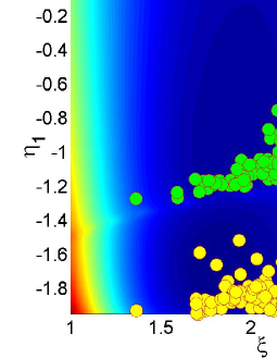
(b) MLE

Figure 2: Top view of (a) the distance metric and (b) the negative log-likelihood function of one realization of the time series with the Gaussian covariance dependence and the parameters values $(\sigma,b)=(10,3)$ for $N=100$, projected onto the $(\eta_{1},\xi)$ plane. The yellow circles represent the locations of optimal values of ($\eta_{1}^{*},\xi^{*}$), obtained from 100 different realizations, calculated by (a) MMoM and (b) MLE. The green circles in (b) represent solutions stuck in local minima.

In Fig. 2(a), the DM function of one realization ($N=100$) is projected onto the parameter space $(\eta_{1},\xi)$. The optimal values $\eta_{1}^{*},\xi^{*}$, obtained from the $100$ realizations are also marked on this plane. The DM has a single minimum in the parameter plane. The estimates of $\eta_{1}^{*}$ tend to spread away from the permissibility boundary at $\eta_{1}=-2,$ producing a skewed distribution with relatively large variance. A similar plot of the NLL function, Fig. 2(b), exhibits two local minima. The optimal values $\eta_{1}^{*},\xi^{*}$, shown in green are obtained using the initial guess $\eta_{1}^{(0)}=-1$, while those in yellow (corresponding to the global minimum) are obtained with $\eta_{1}^{(0)}=-1.7$.

Figure 3: Plots of the true correlation function with the Gaussian dependence and the true parameters $\sigma=10$, $b=3$ (circles), and the Spartan ones using the parameter sets estimated by MMoM (diamonds) and MLE (squares).

For interpolation purposes, the differences in the parameter sets obtained by means of the two methods are practically negligible. In Fig. 3, the Spartan correlation functions obtained with the two sets of parameters are compared with the true (Gaussian) correlation. Near the origin and at intermediate distances, which are crucial for the interpolation, the correlation functions almost coincide. The negative values of $\eta_{1}^{*}$ causes a negative hole in the Spartan correlation at larger distances. This hole is only observed in the Gaussian case due to the short range of the constraints.

Considering the optimization statistics, the value of the DM function ($\sim 10^{-21}$) means an excellent match between the sample and stochastic constraints. The MMoM needs more iterations than the MLE to converge. However, the MMoM CPU time is much lower and almost insensitive to the domain size, while the MLE CPU time grows rapidly with $N$. Since the number of iterations is insensitive to $N$ in both MLE and MMoM, the CPU time per iteration shows similar behavior with increasing $N$ as the total CPU time. For example, for $N=1\,000$ the MMoM is $3\,965$ times faster than the MLE. In the case of the Gaussian model reasonable CPU times are attained for the domain sizes considered. However, the optimization slows down considerably for the other covariance models. This is due to the presence of a long flat valley in the DM and the NLL functions, which extends to large $\eta_{1}\approx 10^{5}$. Convergence requires a high number of iterations, $O(10^{3})$, which, for larger $N,$ is easily manageable by MMoM but too expensive computationally in the case of MLE. Hence, in the following we will use MMoM for parameter inference.

5.2 Results: Interpolation

In the following we investigate the problem of interpolation (missing data prediction). Let us denote by $p$ the degree of thinning, i.e., the percentage of the missing data. We select one time series with $N=1\,000$ per covariance model and we generate $100$ different partitions into a validation set, containing $660$ points at random, and a training set, containing $340$ points (i.e., $p\approx 0.66.$) For comparison purposes, in Fig. 4, we show the $\eta_{1}^{*},\xi^{*}$ estimates for $p=0$ (full data) and the distribution of the $\eta_{1}^{*},\xi^{*}$ values for $p=0.66$, calculated by both the MLE and the MMoM.

Figure 4: Optimal $\eta_{1}^{*},\xi^{*}$ estimates from complete series of 1  000 points calculated by MLE (filled star) and MMoM (filled circle). Also, distribution of the optimal $\eta_{1}^{*},\xi^{*}$ estimates based on the training set of 340 points calculated by MLE (empty stars) and MMoM (empty circles).

We use both KWP (with search neighborhood extending over the entire series) and the Spartan predictor. The covariance function is calculated using the asymptotic formulas given by Eqs. (18). For the analysis of prediction performance, the validation points are segregated into $9$ different categories, based on the number of nearest and next-nearest neighbors that belong in the training set. For example, the category $(i,j),\,i,j=0,1,2,$ includes those validation points for which $i$ nearest neighbors and $j$ second-nearest neighbors are in the training set.

The following statistics are calculated, for each category separately, and over all the validation points: mean absolute error (MAE), mean relative error (MRE), mean absolute relative error (MARE), and root mean square error (RMSE). The calculations are performed for the four covariance models and results for the Gaussian and the exponential cases are shown in Tables 2 and 3. Overall, validation points with more data in their interaction neighborhood display smaller errors than those with fewer data. In the Gaussian and the Whittle-Matérn cases the KWP performs slightly better than the SP, while in the exponential and the spherical cases there is no significant difference between the two methods.

Table 2: SP and KWP performance comparison on synthetic data with Gaussian covariance and parameters: mean $m=50$, standard deviation $\sigma=10$ and correlation length $b=3$. The Spartan parameters were inferred from a training set of $340$ points. The errors were calculated from the validation set of $660$ points.

		(2,2)	(1,2)	(0,2)	(0,1)	(0,0)	(1,1)	(1,0)	(2,0)	(2,1)	Total
MAE	SP	0.40	1.17	3.30	5.36	7.98	1.89	2.93	0.90	0.64	3.83
	KWP	0.27	0.96	3.17	5.15	7.85	1.72	2.86	0.86	0.52	3.69
MARE [%]	SP	0.8	2.5	7.0	11.5	17.4	4.0	6.2	1.9	1.3	8.2
	KWP	0.6	2.0	6.7	10.9	17.1	3.6	6.0	1.8	1.1	7.9
MRE [%]	SP	$-$0.1	$-$0.2	$-$1.1	$-$1.7	$-$4.0	$-$0.4	$-$0.5	$-$0.2	$-$0.1	$-$1.3
	KWP	0.0	$-$0.1	$-$0.9	$-$1.5	$-$3.9	$-$0.3	$-$0.5	$-$0.1	$-$0.1	$-$1.3
RMSE	SP	0.49	1.46	4.13	7.25	10.28	2.42	3.82	1.15	0.84	6.03
	KWP	0.32	1.21	3.98	6.43	9.62	2.16	3.61	1.10	0.66	5.51

Table 3: SP and KWP performance comparison on synthetic data with exponential covariance and parameters: mean $m=50$, standard deviation $\sigma=10$ and correlation length $b=5$. The Spartan parameters were inferred from a training set of $340$ points. The errors were calculated from the validation set of $660$ points.

		(2,2)	(1,2)	(0,2)	(0,1)	(0,0)	(1,1)	(1,0)	(2,0)	(2,1)	Total
MAE	SP	3.81	4.08	4.87	5.72	6.76	4.33	4.49	3.60	3.66	5.03
	KWP	3.84	4.11	4.87	5.71	6.75	4.36	4.49	3.61	3.68	5.04
MARE [%]	SP	8.0	8.6	10.4	12.3	14.6	9.2	9.6	7.6	7.8	10.8
	KWP	8.0	8.7	10.4	12.3	14.6	9.3	9.6	7.6	7.8	10.8
MRE [%]	SP	$-$0.3	$-$1.1	$-$1.7	$-$2.4	$-$3.0	$-$1.3	$-$1.6	$-$0.8	$-$1.0	$-$1.8
	KWP	$-$0.2	$-$1.1	$-$1.7	$-$2.3	$-$3.0	$-$1.2	$-$1.5	$-$0.7	$-$1.0	$-$1.8
RMSE	SP	4.58	5.11	6.08	7.18	8.46	5.38	5.59	4.46	4.55	6.44
	KWP	4.62	5.15	6.08	7.17	8.46	5.40	5.59	4.46	4.58	6.44

6 Case Study II: Aerosol concentration data

Next, we consider an application of the Spartan predictor to a time series consisting of concentration measurements of atmospheric aerosol PM2.5 particles (i.e., particles of aerodynamic diameter smaller than $2.5\mu m$). These measurements were sampled on the grounds of the Technical University of Crete using the aerosol monitor DustTrak, over a period of almost $10$ days in June 2006. The original time series consists of $2\,831$ mean concentration values, measured at $5$ minute intervals. The correlations in the observed series span over large distances (measured in the lag of $\alpha=5$ minutes). In order to make the interpolation task more challenging, we reduced the length of the series by non-overlapping clustering the original data using averages over $\alpha=40$ minute intervals. This resulted in a coarse-grained time series of $353$ data points that will be used below. The data fail the Kolmogorov-Smirnov normality test at the $5\%$ level. Nonetheless, in the following we will model the series with a second-order stationary FGC Spartan random process. The motivation for this approach is that reasonable interpolation performance can be obtained by matching the short-range correlations.

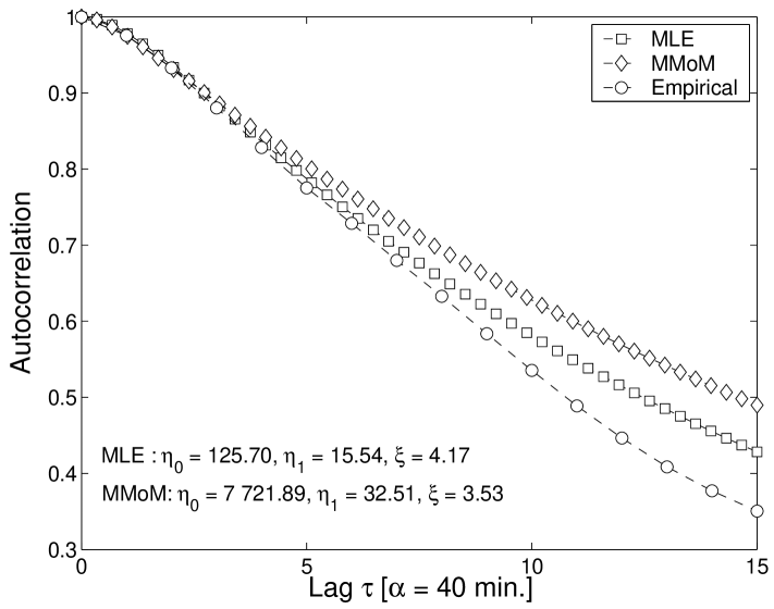
Figure 5: Plots of the empirical correlation function of the aerosol concentration data (circles), and the Spartan ones using the parameters estimated by MMoM (diamonds) and MLE (squares). The lag is measured in units of the sampling step $\alpha=40$ min.

Table 4: Spartan model parameters $\eta_{0}^{*}$, $\eta_{1}^{*}$ and $\xi^{*}$, number of optimization iterations, $N_{it}$, the optimization CPU time, $T_{cpu}$, and the final value $F^{*}$ of the objective function (NLL for MLE and DM for MMoM), calculated from the complete aerosol concentration time series by MLE and MMoM.

	$\eta_{0}^{*}$	$\eta_{1}^{*}$	$\xi^{*}$	$N_{it}$	$T_{cpu}[s]$	$F^{*}$
MLE	5 213.90	15.54	4.17	76.00	16.03	585.89
MMoM	7 721.90	32.51	3.53	182.00	0.39	2E$-29$

The Spartan parameters based on the complete time series are shown in Table 4). The number of iterations involved in the MMoM is more than twice as high as that for the MLE, but the CPU time is $41$ times faster. The final DM value of $F^{*}=2\,10^{-29}$ indicates excellent matching between the sample and stochastic constraints. In Fig. 5, we compare the correlation functions based on the estimated Spartan parameters with the experimental correlation. Very good agreement of the experimental and estimated functions at short time ranges is observed.

Table 5: SP and KWP performance comparison on the aerosol concentration data. The Spartan parameters were inferred by MLE, using the training set of 121 points and the errors were calculated on the validation set of the remaining 232 points. Category $(i,j)$ includes points with $i$ nearest and $j$ next-nearest neighbors from the training set.

		(2,2)	(1,2)	(0,2)	(0,1)	(0,0)	(1,1)	(1,0)	(2,0)	(2,1)
MAE	SP	1.75	2.67	3.85	5.30	8.15	2.88	3.24	2.05	2.03
	KWP	1.80	2.68	3.87	5.32	8.10	2.90	3.25	2.06	2.06
MARE [%]	SP	4.3	6.6	9.3	12.5	19.1	6.8	7.5	4.5	4.9
	KWP	4.4	6.7	9.4	12.6	19.0	6.9	7.6	4.5	5.0
MRE [%]	SP	$-$0.4	$-$1.1	$-$1.4	$-$2.6	$-$5.2	$-$0.9	$-$0.9	$-$0.2	$-$0.8
	KWP	$-$0.4	$-$0.9	$-$1.3	$-$2.5	$-$5.0	$-$0.8	$-$0.8	$-$0.2	$-$0.6
RMSE	SP	2.15	3.72	5.14	7.44	11.04	4.23	4.65	2.92	2.93
	KWP	2.19	3.73	5.12	7.46	10.97	4.25	4.65	2.92	2.98

For the interpolation, the data are partitioned into a training set that involves $121$ randomly selected times, and a validation set including the remaining $232$ values. The parameter inference on the training set is performed by both MMoM and MLE. There is no multimodality in either NLL or DM surface. However, as shown in Fig. 6, there is considerable scatter in the parameter estimates obtained from different training set realizations.

(a) MMoM

(b) MLE

Figure 6: Top view of (a) the distance metric and (b) the negative log-likelihood function of the complete aerosol concentration time series, projected onto the $(\eta_{1},\xi)$ plane. The yellow circles represent the locations of optimal values of ($\eta_{1}^{*},\xi^{*}$), obtained from the complete data and the yellow stars those obtained from 100 different realizations of the training set of 121 points, calculated by (a) MMoM and (b) MLE (a few points are out of the scale range).

We calculate the same interpolation error measures as for the synthetic data. The results are shown in Table 5, using MLE estimates of the Spartan parameters. The differences between the SP and the KWP are minimal. The estimates obtained using the MLE based Spartan parameters are slightly better than the ones based on the MMoM. For comparison, the total mean absolute relative error of the MLE-based estimates is only $0.8\%$ (using the Spartan predictor) and $0.9\%$ (using the KWP) smaller than the MMoM one.

Figure 7: Aerosol concentration time series reconstruction for one training set realization of 121 points. The data in training set are marked by empty circles. The data in the validation set are marked by crosses. The estimates at the validation set locations are marked by filled circles. The time unit is $\alpha=40$ minutes.

In Fig. 7, we illustrate the missing data reconstruction based on the Spartan predictor. As the data in Table 5 already suggest, the largest deviations of the estimates from the actual data are seen in the cases of ”isolated” points with no training data in their interaction neighborhood, i.e., in the category (0,0). The contribution to the total errors from such points can be considerable if the missing data represent a large portion of the entire series. In Table 6, the total errors are shown versus the percentage of the missing data. The mean values of the correlation coefficient ($R$) between the estimated and actual values at the missing points is also included. High correlation values $(\approx 95\%)$ are observed even for $p=0.66$.

Table 6: SP and KWP performance comparison based on the aerosol concentration time series for different sizes of missing data. The Spartan parameters are inferred by MMoM using training sets of $(1-p)*N$ points. The errors are calculated based on the remaining $p*N$ points, for $N=353$ and $p=0.66,0.6,0.4,0.2$.

	$p$	0.66	0.60	0.40	0.20
MAE	SP	4.66	3.86	2.81	2.05
	KWP	4.69	3.85	2.81	2.00
MARE [%]	SP	11.1	9.1	6.6	5.6
	KWP	11.2	9.1	6.6	5.4
MRE [%]	SP	$-$2.6	$-$1.7	$-$0.7	$-$1.2
	KWP	$-$2.5	$-$1.6	$-$0.8	$-$1.0
RMSE	SP	7.18	6.00	4.34	3.07
	KWP	7.25	5.98	4.34	2.97
$R$	SP	0.95	0.97	0.99	0.99
	KWP	0.95	0.97	0.99	0.99

7 Conclusions

We present a framework for the analysis of Gaussian, stationary time series based on Spartan random processes. In this framework, the temporal dependence is determined from ‘pseudo-energy’ functionals. The modified method of moments (MMoM) is proposed for Spartan parameter estimation. Its main advantages are low computational complexity (high speed) even for large sample sizes. Temporal interpolation is formulated by maximizing the conditional probability density function of the Spartan process, based on the available data. The method is tested with synthetic data and with a time series of atmospheric PM2.5 aerosol concentration. The Spartan interpolator is shown to perform similarly to the standard Kolmogorov-Wiener predictor at reduced computational cost.

In time series modeling, it is often necessary to treat the model parameters as time-dependent and to estimate them continuously in the ”moving window” fashion. This approach accounts for lack of stationarity, which is a common feature in meteorological data. The ”moving window” approach has been recently applied to the automatic mapping of rainfall data, using maximum likelihood for parameter inference and universal kriging as the interpolator (Pardo-Iguzqúiza et al.,, 2005). Windows are typically overlapping and of varying size. In each window, parameter inference and model selection (based on the Akaike Information Criterion) are conducted, followed by interpolation. Spartan random processes have definite advantages for application in the moving window framework. First, model selection can be bypassed thanks to the flexibility of the SRP (compared with two or three parameter covariance models). Second, the computational efficiency of Spartan parameter inference and interpolation would allow for iterative methods of window size adjustment that will properly account for the physical conditions at the local scale.

List of figures

Fig 1: Some trivial time series, consisting of only 3 points, for which equivalence between SP and KWP can be shown analytically. The circles denote the known data and the crosses the prediction points.

Fig 2: Top view of (a) the distance metric and (b) the negative log-likelihood function of one realization of the time series with the Gaussian covariance dependence and the parameters values $(\sigma,b)=(10,3)$ for $N=100$, projected onto the $(\eta_{1},\xi)$ plane. The yellow circles represent the locations of optimal values of ($\eta_{1}^{*},\xi^{*}$), obtained from 100 different realizations, calculated by (a) MMoM and (b) MLE. The green circles in (b) represent solutions stuck in local minima.

Fig 3: Plots of the true correlation function with the Gaussian dependence and the true parameters $\sigma=10$, $b=3$ (circles), and the Spartan ones using the parameter sets estimated by MMoM (diamonds) and MLE (squares).

Fig 4: Optimal $\eta_{1}^{*},\xi^{*}$ estimates from complete series of 1  000 points calculated by MLE (filled star) and MMoM (filled circle). Also, distribution of the optimal $\eta_{1}^{*},\xi^{*}$ estimates based on the training set of 340 points calculated by MLE (empty stars) and MMoM (empty circles).

Fig 5: Plots of the empirical correlation function of the aerosol concentration data (circles), and the Spartan ones using the parameters estimated by MMoM (diamonds) and MLE (squares). The lag is measured in units of the sampling step $\alpha=40$ min.

Fig 6: Top view of (a) the distance metric and (b) the negative log-likelihood function of the complete aerosol concentration time series, projected onto the $(\eta_{1},\xi)$ plane. The yellow circles represent the locations of optimal values of ($\eta_{1}^{*},\xi^{*}$), obtained from the complete data and the yellow stars those obtained from 100 different realizations of the training set of 121 points, calculated by (a) MMoM and (b) MLE (a few points are out of the scale range).

Fig 7: Aerosol concentration time series reconstruction for one training set realization of 121 points. The data in training set are marked by empty circles. The data in the validation set are marked by crosses. The estimates at the validation set locations are marked by filled circles. The time unit is $\alpha=40$ minutes.

References

- Adler, (1981) Adler, R.J., 1981. The Geometry of Random Fields. Wiley. New York.
- Ballesta, (2005) Ballesta, P.P., 2005. The uncertainty of averaging a time series of measurements and its use in environmental legislation. Atmospheric Environment 39, 2003-2009.
- Bochner, (1959) Bochner, S., 1959. Lectures on Fourier Integrals. Princeton University Press. Princeton, NJ.
- Byron et al., (1992) Byron, F.W. Jr., Fuller, R.W., 1992. Mathematics of Classical and Quantum Physics. Dover. NY.
- Elogne et al., (2008) Elogne, S. N., Hristopulos, D.T., and Varouchakis, E., 2008. An Application of Spartan Spatial Random Fields in Environmental Mapping: Focus on Automatic Mapping Capabilities. Stochastic Environmental Research and Risk Assessment 22(5), in press. [Online] DOI:10.1007/s00477-007-0167-5.
- Gradshteyn et al., (1980) Gradshteyn, I.S., Ryzhik, I.M., 1980. Table of Integrals, Series and Products, edition. Academic Press. San Diego.
- Hopke et al., (2001) Hopke, P.K., Liu, C., Rubin, D.B., 2001. Multiple Imputation for Multivariate Data with Missing and Below-Threshold Measurements: Time-Series Concentrations of Pollutants in the Arctic. Biometrics 57, 22-33.
- Houseman, (2005) Houseman, E.A., 2005. A robust regression model for a first-order autoregressive time series with unequal spacing: application to water monitoring. Applied Statistics 54(4), 769-780.
- Hristopulos, (2003) Hristopulos, D.T., 2003. Spartan Gibbs random field models for geostatistical applications. SIAM Journal in Scientific Computation 24, 2125-2162.
- Hristopulos and Elogne, (2007) Hristopulos D. T., and Elogne, S. 2007. Analytic properties and covariance functions for a new class of generalized gibbs random fields. IEEE Transactions on Information Theory 53(12), 4467-4679.
- Johnson, (2004) Johnson, M.E., 1987. Multivariate Statistical Simulation. John Wiley. NY.
- Junninen et al., (2004) Junninen, H., Niska, H., Tuppurainen, K., Ruuskanen J., Kolehmainen, M., 2004. Methods for imputation of missing values in air quality data sets. Atmospheric Environment 38, 2895-2907.
- Kitanidis, (1997) Kitanidis, P.K., 1997. Introduction to Geostatistics: Applications to Hydrogeology. Cambridge.
- Paatero et al., (2005) Paatero, P., Aalto, P., Picciotto, S., Bellander, T., Castano-Vinyals, G., Cattani, G., Cyrys, J., Kulmala, M., Lanki, T., Nyberg, F., et al., 2005. Estimating time series of aerosol particle number concentrations in the five HEAPSS cities on the basis of measured air pollution and meteorological variables. Atmospheric Environment 39, 2261-2273.
- Pardo-Iguzqúiza et al., (2005) Pardo-Iguzqúiza, E., Dowd, P.A., Grimes, D.I.F., 2005. An automatic moving window approach for mapping meteorological data. International Journal of Climatology 25, 665-678.
- Press et al., (1992) Press, W.H., Teukolsky, S.A., Vettering, W.T., Flannery, B.P., 1992. Numerical Recipes in Fortran, Vol. 1. Cambridge University Press. New York.
- Reusken, (2002) Reusken, A., 2002. Approximation of the determinant of large sparse symmetric positive definite matrices. SIAM J. Matrix Anal. Appl. 23, 799-818.
- Smelyanskiy et al., (2005) Smelyanskiy, V. N., Luchinsky, D. G., Timuçin, D. A., Bandrivskyy, A., 2005. Reconstruction of stochastic nonlinear dynamical models from trajectory measurements, Phys. Rev. E, 72(2), 026202.
- Stein, (1999) Stein, M. L., 1999. Interpolation of Spatial Data. Some Theory for Kriging. Springer, New York.
- Wackernagel, (2003) Wackernagel, H., 2003. Multivariate Geostatistics. Springer. Berlin.
- Yaglom, (1987) Yaglom, M., 1987. Correlation Theory of Stationary and Related Random Functions I. Springer. New York.