Multifractal Distribution of Dendrite on One-dimensional Support

Abstract

We apply multifractal analysis to an experimentally obtained quasi-two-dimensional crystal with fourfold symmetry, in order to characterize the sidebranch structure of a dendritic pattern. In our analysis, the stem of the dendritic pattern is regarded as a one-dimensional support on which a measure is defined and the measure is identified with the area, perimeter length, and growth rate distributions. It is found that these distributions have multifractality and the results for the area and perimeter length distributions, in the competitive growth regime of sidebranches, are phenomenologically understood as a simple partitioning process.

1 Introduction

It has been well established that a dendritic pattern is typical in crystal growth. Its growth process is dominated by diffusion and anisotropy [1] and consists of several stages; (i) A tip grows stably and steadily, and a straight stem is formed. The stability of the tip is attributed to anisotropy. (ii) Sidebranches are generated behind the tip due to noise effects[2] and the instability of a flat interface [3]. (iii) Sidebranches grow competing mutually. This competition is known as one of the most characteristic and interesting properties in growth dominated by diffusion. A longer sidebranch screens off the diffusional field and suppresses the growth of shorter ones around it. This process occurs on various length scales. As a result, complicated and hierarchical structures are formed. (iv) Finally, surviving branches grow independently.

Our aim in this paper is to characterize the sidebranch structure (at stages (ii) and (iii))of a dendritic pattern. It is interesting and worth considering since the sidebranch structure determines the outline of the pattern. Many types of scaling analysis based on scaling idea have been attempted. One concerns the properties of global structure constructed by sidebranches. For the pattern of a three-dimensional dendritic crystal projected onto a two-dimensional plane, it has been reported [4, 5, 6] that $S(X)\sim X^{\delta_{S}}$ and $L(X)\sim X^{\delta_{L}}$ with $\delta_{S}\sim\delta_{L}\sim 1.7$, where $S$ is the area of the pattern and $L$ the perimeter length up to $X$, which is the distance along the stem from the tip. Interestingly, for the pattern of a quasi-two-dimensional crystal, $S(X)\sim X^{\delta_{S}}$ with $\delta_{S}\sim 1.5$[7]. Active sidebranches, whose growth is not suppressed by the screening effect of a longer sidebranch, form the envelope $Z(X)$ of the pattern, where $Z(X)$ denotes the height from the stem at $X$. The envelope is constructed by connecting the tips of active sidebranches and obeys the power law $Z(X)\sim X^{\kappa}$[5, 6, 8]. It has been observed that $\kappa<1$ near behind the tip and $\kappa>1$ far from the tip[9]. Another scaling analysis concerns the growth of an individual sidebranch or the statistical properties of a set of sidebranches. In the competing growth of sidebranches, each branch grows as $h_{j}(t_{j})\sim t_{j}^{\sigma_{j}}$, with $\sigma_{j}\sim 0.5-0.7$, where $h_{j}(t_{j})$ is the height of the $j$-th branch at $t_{j}$, the time from its birth, and subsequently the growth decays exponentially[10]. For a set of sidebranches it is found that the height distribution $N(h)$ obeys the following power law, $N(h)\sim h^{-\beta}$, with $\beta\sim 2.2$[11].

In this paper we present a new characterization of the sidebranch structure of a dendritic pattern using multifractal formalism. Since the stem of a dendritic pattern grows straight, it can be considered as a one-dimensional support on which a probability measure is defined. We apply this approach to an experimentally obtained quasi-two-dimensional dendritic pattern of an ${\rm NH_{4}Cl}$ crystal. The crystal is obtained from a supersaturated solution and has fourfold symmetry. We identify the probability measure with the area and perimeter length distributions of the pattern and the growth rate distribution at the interface. In the competitive growth of sidebranches, the solute particles diffusing in the solvent are distributed unequally to branches since it is easy to reach the tip of longer branches whereas it is difficult to reach the shorter branches between longer ones. This process is expected to occur on various length scales, similar to energy dissipation in turbulence, which is simply modeled by the ”binomial branching process”[12] and shows multifractality. As for the growth rate distribution on the interface, it is known to have multifractality with the interface itself as a (fractal) support[13]. Therefore we expect multifractality in our point of view here.

The rest of the paper is organized as follows: In section 2 our crystallization experiment is briefly described. The multifractal formulation is given in section 3. The binomial branching process is introduced and the results of multifractal analysis are referred to. In section 4 our results and discussion are given. For the area and perimeter length distributions, comparison with those for the binomial branching process are presented. Section 5 is dedicated to the summary and future outlook.

2 Experiment

We analyze a quasi-two-dimensional dendritic pattern, with well-developed sidebranches and a clear envelope, obtained from an ${\rm NH_{4}Cl}$ solution growth experiment. The details of the experiment are described in our previous articles[11]: An ${\rm NH_{4}Cl}$ aqueous solution saturated at approximately 40 ${}^{\circ}{\rm C}$ is sealed in a Hele-Shaw cell, which has a small gap between two glass plates placed in parallel. The thickness of the gap is 100 $\mu$m. Then when the temperature is lowered to approximately 30 ${}^{\circ}{\rm C}$, the solution becomes supersaturated and nucleation takes place. The direction of the tip growth is $\langle$100$\rangle$ in the supersaturated solution. Sidebranches grow perpendicularly to the stem, with small sub-sidebranches perpendicular to them. The observed tip velocity $v_{\rm tip}$ is 40$-$49 $\mu$m/sec. The diffusion length of the tip, $l_{\rm D}=2D/v_{\rm tip}$, where $D$ is the diffusion constant of ${\rm NH_{4}Cl}$ ($2.6\times 10^{3}\mu{\rm m}^{2}/{\rm s}$[14]), is larger than the thickness of the cell. Therefore the growth is considered to be quasi-two-dimensional. The image of the crystal is obtained by using a microscope and charge-coupled device (CCD) camera and is binarized by an image processing. The image of a crystal is shown in Fig. 1, whose resolution is $640\times 480$ pixels.

Figure 1: Image of a dendritic crystal. The resolution is 640$\times$480 pixels. For our analysis, the $X$-axis is set along the stem with the tip on it. The $Z$-axis is set parallel to the sidebranches. The pattern is covered with strips of width $\epsilon$ aligned parallel to the $Z$-axis. There is no correlation between the sidebranch patterns of $Z\geq 0$ and $Z\leq 0$.

3 Multifractal

3.1 Formulation: on one-dimensional support

Suppose that the stem of a dendrite grows along the $X$-axis, with the tip on the $X$-axis, and the sidebranches grow in the positive and negative $Z$ directions (see Fig. 1). There is no correlation between the growths in the positive and negative $Z$ regions[2]. Therefore each pattern can be dealt with as an independent sample.

Consider that a pattern (for example, the pattern shown in Fig. 1, $Z\geq 0$) is covered with disjoint strips of width $\epsilon$ aligned parallel to the $Z$-axis, as shown in FIG.1. Let $p_{j}(\epsilon)$ be a measure (nonnegative scalar quantity) assigned to the $j$-th strip. The measure is normalized to be a probability

$$\sum_{j=1}^{N(\epsilon)}p_{j}(\epsilon)=1,$$ (1)

where $N(\epsilon)$ is the number of strips necessary to cover the pattern completely. In our point of view, the stem is regarded as a one-dimensional support on which the probability measure is defined.

The partition function $Z(q,\epsilon)$ is defined by the probability measure as

$$Z(q,\epsilon)=\sum_{j,p_{j}(\epsilon)\neq 0}[p_{j}(\epsilon)]^{q}.$$ (2)

Based on the expectation that for small $\epsilon$ the scaling law $Z(q,\epsilon)\sim\epsilon^{\tau(q)}$ holds, the multifractal exponent $\tau(q)$ is defined as

$$\tau(q)=\lim_{\epsilon\rightarrow 0}\frac{\log Z(q,\epsilon)}{\log\epsilon}.$$ (3)

Practically $\tau(q)$ is evaluated from the slope of $\log Z(q,\epsilon)$ versus $\log\epsilon$. Then the generalized dimension $D(q)$ is defined as[15]

$$D(q) = \frac{1}{q-1}\tau(q),\quad{\rm for}\quad q\neq 1,$$ (4)

$$D(1) = \frac{d}{dq}\tau(q)|_{q=1}$$ (5)

$$= \lim_{\epsilon\rightarrow 0}\frac{\sum_{j}p_{j}(\epsilon)\log p_{j}(\epsilon)}{\log\epsilon},\quad{\rm for}\quad q=1.$$

Using the Legendre transformation the singularity exponent $\alpha$ and its fractal dimension $f(\alpha)$ are given as functions of $q$ as[16]

$$\alpha(q) = \frac{d\tau(q)}{dq},$$ (6)

$$f(\alpha(q)) = q\alpha(q)-\tau(q).$$ (7)

However, it is not useful to numerically evaluate $\alpha$ and $f(\alpha)$ from Eqs. (6) and (7), since they may produce relatively large errors. Therefore instead, we adopt the direct method described below[17].

Let us construct a new probability measure $\mu_{j}(\epsilon,q)$ with parameter $q$ from $p_{j}(\epsilon)$ as

$$\mu_{j}(\epsilon,q)=\frac{\{p_{j}(\epsilon)\}^{q}}{\sum^{N({\epsilon})}_{j}\{p_{j}(\epsilon)\}^{q}}.$$ (8)

Then let us define $\zeta(\epsilon,q)$ and $\xi(\epsilon,q)$ as

$$\zeta(\epsilon,q) = \sum_{j}\mu_{j}(\epsilon,q)\log[p_{j}(\epsilon)],$$ (9)

$$\xi(\epsilon,q) = \sum_{j}\mu_{j}(\epsilon,q)\log[\mu_{j}(\epsilon,q)].$$ (10)

From them $\alpha$ and $f(\alpha)$ are given as functions of $q$ as

$$\alpha(q) = \lim_{\epsilon\rightarrow 0}\frac{\zeta(\epsilon,q)}{\log\epsilon},$$ (11)

$$f(q) = \lim_{\epsilon\rightarrow 0}\frac{\xi(\epsilon,q)}{\log\epsilon}.$$ (12)

Practically they are evaluated from the slopes of $\zeta(\epsilon,q)$ and $\xi(\epsilon,q)$ versus $\log\epsilon$, respectively. Direct calculation shows that the definitions (11) and (12) satisfy the relations (6) and (7).

3.2 Binomial branching process

We refer to the binomial branching process[12] for our later consideration. It shows multifractality and fortunately the multifractal spectrum can be exactly calculated due to its simplicity.

Figure 2: (a) Different stages of the binomial branching process. Each segment is divided into two equal subsegments at the next stage. The measure is divided into nonequal fractions, $p$ and $(1-p)$. (b) $f(\alpha)$ spectrum of the binomial branching process with $p=0.7$.

Suppose that a segment of length 1 is divided into two segments of length 1/2. A probability measure $p$ $(>1/2)$ is assigned to the left segment and $(1-p)$ to the right. This $p$ is the only adjustable parameter of the process. Next, each segment is subdivided into two equal halves and the measure is partitioned into $p$ to the left half and $(1-p)$ to the right. So there are four segments of length 1/4 and the measures $p^{2}$, $p(1-p)$, $(1-p)p$ and $(1-p)^{2}$ are assigned to the segments from left to right. This procedure is repeated again and again (see Fig. 2, we can see a similarity between the $n=8$ pattern and the sidebranch structure shown in Fig. 1). At the $n$-th iteration, there are $2^{n}$ segments of length $2^{-n}$ and the number of segments with measure $p^{k}(1-p)^{n-k}$, $k=0,1,\cdots,n$, is $\binom{n}{k}=n!/[k!(n-k)!]$. Therefore the partition function of the stage, $Z(q,n)\equiv Z(q,\epsilon)$ where $\epsilon=2^{-n}$, is immediately calculated as

$$Z(q,n) = \sum_{k=0}^{n}\left(\begin{array}[]{c}n\\ k\end{array}\right)[p^{k}(1-p)^{n-k}]^{q}$$ (15)

$$= [p^{q}+(1-p)^{q}]^{n}.$$ (16)

Then the exponent $\tau(q)$ can be obtained as

$$\tau(q)=-\frac{\log[p^{q}+(1-p)^{q}]}{\log 2}.$$ (17)

Using the Legendre transformation the singularity exponent and the fractal dimension are calculated as

$$\alpha(q)=-\frac{\eta\log p+(1-\eta)\log(1-p)}{\log 2},$$ (18)

$$f(\alpha(q))=-\frac{\eta\log\eta+(1-\eta)\log(1-\eta)}{\log 2},$$ (19)

where $\eta=p^{q}/[p^{q}+(1-p)^{q}]$. The direct evaluation using eqs.(11) and (12) gives the same result.

The $f(\alpha)$ spectrum takes a continuous value for $[\alpha_{\rm min},\alpha_{\rm max}]$, where $\alpha_{\rm min}=-\log_{2}p$ and $\alpha_{\rm max}=-\log_{2}(1-p)$. It is symmetric with respect to $\alpha=\alpha(q=0)=-(\log_{2}p+\log_{2}(1-p))/2$ and takes the maximum at $\alpha=\alpha(q=0)$, $f(\alpha(q=0))=D(0)=1$, reflecting the fact that the support is one-dimensional. The information dimension $D(1)=(\alpha(q=1)=f(\alpha(q=1)))$ is given as

$$D(1)=-\frac{p\log p+(1-p)\log(1-p)}{\log 2}.$$ (20)

4 Results and Discussion

4.1 Area distribution

First of all, we investigate the structure of the area distribution. The area of the pattern is defined as the number of pixels which constitute the pattern.

The generalized dimension $D(q)$ for the pattern shown in Fig. 1, $Z\geq 0$ is shown in Fig. 3. Taking into consideration that each sidebranch has a finite thickness of $\sim$5$-$25 pixels, we use 6 pixels as the minimum of the strip width in our analysis. On the other hand we use 120 pixels as the maximum. The exponent $\tau(q)$ is obtained by least squares method. The log-log plots of $Z(q,\epsilon)$ against the strip width $\epsilon$ and the fitting lines for some values of $q$ are shown in Fig.4. The scaling relation holds quite well.

Figure 3: Generalized dimension $D(q)$ of the area distribution for the pattern shown in Fig. 1, $Z\geq 0$, and that for the binomial branching process with $p=0.68$. The error bars are obtained from the data of 30 samples.

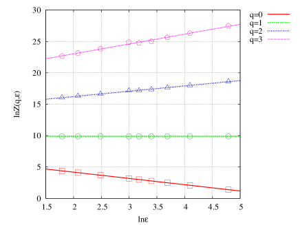
Figure 4: (Color online) Log-log plots of $Z(q,\epsilon)$ of the area distribution for the pattern shown in Fig. 1, $Z\geq 0$, against strip width $\epsilon$, for $q=$0, 1, 2, and 3. The slope gives the exponent $\tau(q)$. For the ease of viewing, the measure is not normalized to be a probability, i.e., $Z(q=1,\epsilon)$ is the total area of the pattern.

The multifractal $f$-$\alpha$ spectrum for the same pattern is shown in Fig. 5, along with that for the binomial branching process. The maximum of $f(\alpha)$ equals 1, since the support is one-dimensional. The spectrum is evaluated using eqs. (8)$-$(12). The plots of $\zeta(q,\epsilon)$ and $\xi(q,\epsilon)$ against $\log\epsilon$ and least squares fitting are shown in Fig. 6. The fitting gives considerably good evaluations, although there exist some scattering points for larger $q$.

Figure 5: $f$-$\alpha$ spectrum of the area distribution for the pattern shown in Fig. 1, $Z\geq 0$, and for the binomial branching process with $p=0.68$. The error bars are obtained from the data of 30 samples.

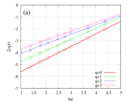
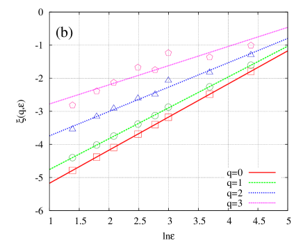
Figure 6: (Color online) Fitting of $\alpha$ and $f$ for $q=$0, 1, 2, and 3. (a) Plots of $\zeta(q,\epsilon)$ of the area distribution for the pattern shown in Fig.1, $Z\geq 0$, and (b) plots of $\xi(q,\epsilon)$ against $\ln\epsilon$.

It is found that both $D(q)$ and the $f$-$\alpha$ spectrum take continuous values dependent on $q$ and $\alpha$, respectively, within the range between $D(q\rightarrow\infty)=\alpha_{\rm min}\sim 0.56$ and $D(q\rightarrow-\infty)=\alpha_{\rm max}\sim 1.7$. This finding indicates that the area distribution has multifractality. Multifractality characterizes the pattern in more detail than the global scaling relations mentioned in the Introduction by using a local scaling relation and distributions. That is, under the condition of the global scaling relation $S(X)\sim X^{\delta_{S}}$ (see the Introduction), at around a certain point the area scales locally as $\sim\epsilon^{\alpha}$ ($\epsilon\rightarrow 0$) and such a point is distributed as $\sim\epsilon^{-f(\alpha)}$. We compare the results with the binomial branching process with $p=0.68$, which gives the same $\alpha_{\rm min}$. There is a good agreement in the positive $q$ or small $\alpha$ region.

The result is almost independent of the pattern size, as long as the pattern is large enough that competitive growth of sidebranches is well-developed. To see this, in Fig. 7 we show the $f(\alpha)$ spectra for the full pattern shown in Fig. 1, $Z\geq 0$, and for the partial patterns from the tip to 75%, 66%, 33%, and 25% of the full pattern. There is little difference between the spectra of the three partial patterns of 100%, 75%, and 66%. These can be considered as sufficiently large samples. However, for the 33% and 25% patterns, the minimum singularity exponent $\alpha_{\rm min}$ is larger than those for the former three patterns. Therefore the small-$\alpha$ part of the spectrum is contributed to by well-developed longer sidebranches and the large-$\alpha$ part by small sidebranches near the tip or deep inside the forest of longer sidebranches.

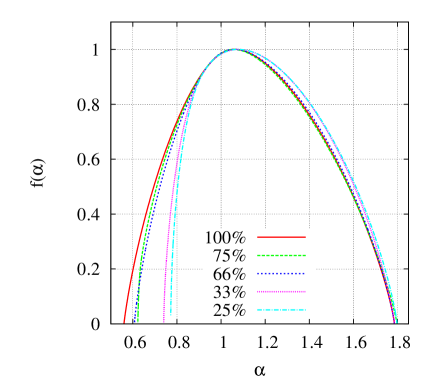
Figure 7: (Color online) Size dependence of the $f$-$\alpha$ spectrum of the area distribution for the patterns shown in Fig.1, $Z\geq 0$.

Our results of some characteristic exponents are summarized in Table. 1, along with those for the binomial branching process with $p=0.68$. They show a good agreement, except for $\alpha_{\rm max}$. Therefore, our phenomenological scenario mentioned in the introduction seems reasonable in the competitive growth regime. However, how the unequal distribution of solute to sidebranches on various length scales is related to the diffusional growth mechanism and how the value $p=0.68$ is derived still remain unclear. On the other hand, there exists some disagreement slightly to the right of the peak of the spectrum This is attributed to the fact that near behind the tip sidebranches are short and growing almost independently, not competing with each other. Note that the reliability of the spectrum for $q<0$ or large $\alpha$ is considerably lower than that for $q>0$ or small $\alpha$ due to the limitation of the resolution.

	$\alpha_{\rm min}$	$\alpha_{\rm max}$	$\alpha(q=0)$	$D(1)$
Area	0.54$\pm$0.06	1.58$\pm$0.11	1.05$\pm$0.02	0.94$\pm$0.03
p=0.68	0.56	1.64	1.10	0.90

Table 1: List of characteristic scaling exponents for the area distribution, along with those for the binomial branching process with $p=0.68$. Note that $\alpha(q=0)$ is the value at which the fractal dimension takes maximum $f=1$. Data are obtained over 30 samples.

4.2 Perimeter length

The perimeter length is defined as the number of pixels which constitute the interface of the pattern. A pixel is said to constitute the interface if it is a part of the pattern and at least one of its four neighboring pixels is not.

Figure 8 shows the generalized dimension $D(q)$ and the $f$-$\alpha$ spectrum for the pattern shown in Fig.1, $Z\geq 0$. It is clear that the distribution has multifractality. Figures 9 and 10 show the log-log plots of $Z(q,\epsilon)$ against $\epsilon$ and the plots of $\zeta(q,\epsilon)$ and $\xi(q,\epsilon)$ against $\log\epsilon$, respectively. They show that the scaling relation holds well.

Figure 8: (a) Generalized dimension and (b)$f$-$\alpha$ spectrum of the perimeter length distribution for the pattern shown in Fig. 1, $Z\geq 0$. The error bars are obtained from the data of 30 samples.

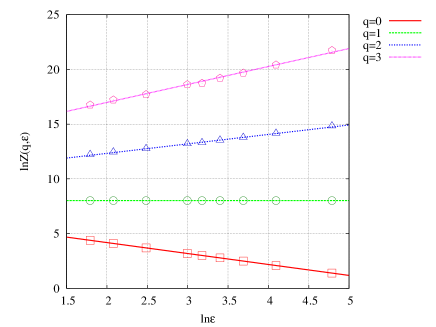
Figure 9: (Color online) Log-log plots of $Z(q,\epsilon)$ of the perimeter length distribution for the pattern shown in Fig. 1, $Z\geq 0$, against the strip width $\epsilon$, for $q=$0, 1, 2, and 3. The measure is not normalized, i.e., $Z(q=1,\epsilon)$ is the total perimeter length of the pattern.

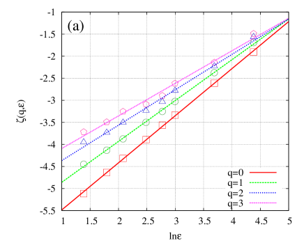
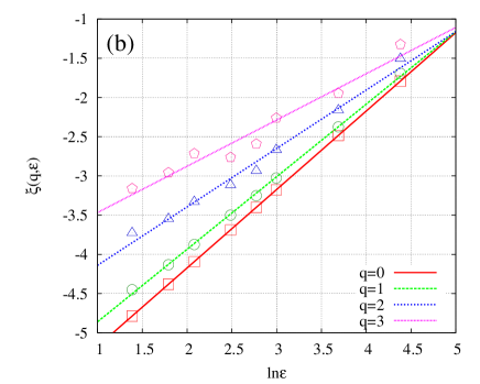
Figure 10: (Color online) Fitting of $\alpha$ and $f$. (a) Plots of $\zeta(q,\epsilon)$ of the perimeter length for the pattern shown in Fig. 1, $Z\geq 0$, and (b) plots of $\xi(q,\epsilon)$ against $\ln\epsilon$ for $q=$0, 1, 2, and 3.

Some characteristic exponents are summarized in Table.2. Note that for some samples $f(\alpha_{\rm max})$ does not equal zero, as shown in Fig.8. For the perimeter length distribution, the number of pixels used in the calculation is considerably smaller than that for the area distribution, since only the pixels constituting the interface of the pattern are to be studied. Due to this fact and the limitation of the resolution, it is quite difficult to obtain a result with satisfactory precision for the $q<0$ or large-$\alpha$ region and to conclude whether $f(\alpha_{\rm max})\neq 0$ or not. It is found that $\alpha_{\rm min}$ for the perimeter length distribution is larger than that for the area distribution. However, there is a good agreement for the values of $\alpha(q=0)$ and $D(1)$ with relatively small error. This is interpreted as follows: $\alpha_{\rm min}$ is dominated by the contribution from long and thick sidebranches only, while both from thick and long, and thin and short sidebranches contribute to $\alpha(q=0)$ and $D(1)$. For thick sidebranches the difference between the number of pixels constituting the branch and that constituting the interface is large, but for thin branches this difference is small. Therefore it is reasonable to assume the same scenario corresponding to the binomial branching process for thin branches as for the area distribution.

	$\alpha_{\rm min}$	$\alpha_{\rm max}$	$\alpha(q=0)$	$D(1)$
Perimeter	0.67$\pm$0.07	1.28$\pm$0.16	1.05$\pm$0.01	0.95$\pm$0.01

Table 2: List of characteristic scaling exponents for the perimeter length distribution. Data are obtained over 30 samples.

4.3 Growth rate distribution

In principle, it is a faithful method to the original data to evaluate the growth rate from the growth area between two successive images. However, for a dendritic pattern such a method is quite difficult to implement with satisfactory precision due to the limitation of the resolution and since the difference of the growth rates between in the fast region and in the slow region is quite large. Therefore instead, we evaluate the growth rate $p({\bf r})$ at point ${\bf r}$ on the interface by numerically solving the Laplace equation $\nabla^{2}\phi({\bf r})=0$ outside of the pattern, where $\phi({\bf r})$ denotes the concentration field, on a square lattice. We set, as a boundary condition, $\phi({\bf r})=Const.$, uniformly on the interface and evaluate the growth rate as the gradient of the concentration field:

$$p({\bf r})\sim|\nabla\phi({\bf r})|.$$ (21)

This evaluation is valid if the diffusion length is larger than the characteristic length of the system - the tip radius of the stem or the average spacing of sidebranch generation - and this is the case: the diffusion length is longer than $100$ $\mu m$ and the characteristic length is of the order of $1$ $\mu m$. We neglect the surface tension effect, since the surface tension effect does not affect the result in the unscreened large growth region[13]. We are intersted in the scaling structure in that region. Then the measure $p_{j}(\epsilon)$ in the $j$-th strip is given as

$$p_{j}(\epsilon)=\sum_{{\bf r}\in j{\rm-th\;strip}}p({\bf r}),$$ (22)

which is normalized to be a probability.

Figure 11 shows the generalized dimension for $q>0$ and the multifractal $f$-$\alpha$ spectrum for small $\alpha$ of the pattern shown in Fig. 1, $Z\geq 0$. The log-log plot of $Z(q,\epsilon)$ against $\epsilon$ and the plots of $\zeta(q,\epsilon)$ and $\xi(q,\epsilon)$ against $\log\epsilon$ are shown in Figs.12 and 13, respectively. Multifractality of the distribution and scaling property are observed. Some characteristic exponents are summarized in Table.3. It is unclear how these values are derived. However, the growth rate distribution considered here is the harmonic measure redefined on a one-dimensional support, which is originally defined on a fractal interface embedded in the two-dimensional plane. Therefore it is expected that our results are closely related to the results for the harmonic measure given on the interface of a dendritic pattern[13]. Particularly it is known that the information dimension for the latter, $D_{f}(1)$, is exactly proved to be 1[18]. We conjecture that there will be a simple relation between the two values of the information dimension, $D(1)=D_{f}(1)/D_{f}(0)=1/D_{f}(0)$ where $D_{f}(0)$($\sim 1.5$) is the fractal dimension of the dendrite interface. This conjecture is based on the assumption that since we consider the same measure on different supports, the interface with the fractal dimension $D_{f}(0)$ and the stem with $D(0)=1$, the two multifractal spectra corresponding to these supports are similar and the condition that they contact the line $f(\alpha)=\alpha$. Our result is consistent with the conjecture within error.

Figure 11: (a) Generalized dimension and (b)$f$-$\alpha$ spectrum of the growth rate distribution for the pattern shown in Fig. 1, $Z\geq 0$. The error bars are obtained from the data of 30 samples.

Figure 12: (Color online) Log-log plots of $Z(q,\epsilon)$ of the growth rate distribution for the pattern shown in Fig. 1, $Z\geq 0$, against the strip width $\epsilon$, for $q=$0, 1, 2, and 3. The measure is not normalized, i.e., $Z(q=1,\epsilon)$ is the total sum of the growth rates.

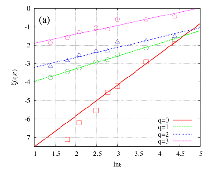
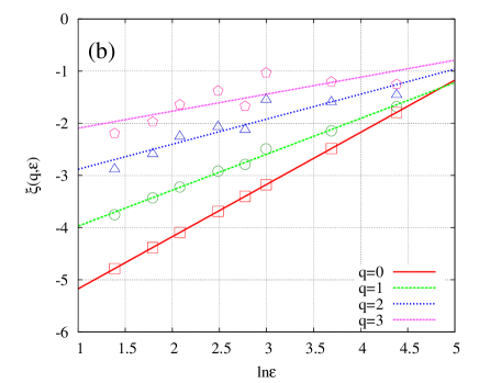
Figure 13: (Color online) Fitting of $\alpha$ and $f$. (a) Plots of $\zeta(q,\epsilon)$ of the growth rate distribution for the pattern of Fig.1, $Z\geq 0$, and (b) plots of $\xi(q,\epsilon)$, against $\ln\epsilon$ for $q=$0, 1, 2, and 3.

$\alpha_{\rm min}$	$\alpha(q=0)$	$D(1)$
0.3$\pm$0.1	1.6$\pm$0.2	0.70$\pm$0.06

Table 3: List of characteristic singular exponents for the growth rate distribution. Data are obtained over 30 samples.

The small-$\alpha$ region is contributed to from unscreened active growth. In our situation there are two domains where growth is active: one is around the tip of longer sidebranches and the other is near behind the tip of the stem, where small short branches are growing almost independently. Therefore, the results for the growth rate distribution are different from those for the area and perimeter length distributions due to the difference of the structure of contribution. For example, short branches contribute to the small-$\alpha$ part of the spectra of the area and perimeter length distributions. On the other hand, for the growth rate distribution, active short branches near behind the tip contribute to the small-$\alpha$ part but frozen ones deep inside the forest of longer branches to the large-$\alpha$ part, which is not discussed here.

5 Summary and Outlook

In order to characterize the sidebranch structure of a dendritic pattern we applied multifractal formalism to the fourfold pattern of an NH₄Cl quasi-two-dimensional crystal, regarding the stem as a one-dimensional support on which the probability measure is given. Multifractality of the area and perimeter length distributions was manifested and was well understood phenomenologically as the binomial branching process. Furthermore the growth rate distribution also showed multifractality from the point of view on one-dimensional support.

There are some problems for further understanding. One concerns the relation between diffusional the growth mechanism and the binomial branching process, which we use to phenomenologically understand the result. It will provide a strong support to our consideration if it is clarified. Another concerns higher multifractality. Since the growth rate is originally given on the interface, it seems natural to consider a measure which has multifractality and is defined on a support which also has multifractality. To our knowledge, the study of such a system has not been carried out in detail, except for the cases of certain simple models[19]. In this point of view the stem is considered as a one-dimensional base space on which the support is distributed. At a certain point on this one-dimensional base space, it is expected that the support locally scales as $\sim\epsilon^{\alpha_{1}}$ and the measure also locally scales as $\sim\epsilon^{\alpha_{2}}$. Such a point is distributed as $\sim\epsilon^{-F(\alpha_{1},\alpha_{2})}$, where $F(\alpha_{1},\alpha_{2})$ is a function of both $\alpha_{1}$ and $\alpha_{2}$. We hope that useful information will be derived from $F(\alpha_{1},\alpha_{2})$, which will enable a more detailed understanding of the sidebranch structure.

- [1] J. S. Langer: Rev. Mod. Phys. 52 (1980) 1.
- [2] A. Dougherty, P. D. Kaplan and J. P. Gollub: Phys. Rev. Lett. 58 (1987) 1652.
- [3] W. W. Mullins and R. F. Sekerka: J. Appl. Phys. 34 (1963) 323; J. Appl. Phys. 35 (1964) 444.
- [4] E. Hurlimann, R. Trittibach, U. Bisang and J. H. Bilgram: Phys. Rev. A 46 (1992) 6579.
- [5] Q. Li and C. Beckermann: Phys. Rev. E 57 (1998) 3176.
- [6] A. Dougherty and R. Chen: Phys. Rev. A 46 (1992) R4508.
- [7] Y. Couder, F. Argoul, A. Arneodo, J. Maurer and M. Rabaud: Phys. Rev. A 42 (1990) 3499.
- [8] Y. Corrigan, M. B. Koss, J. C. LaCombe, K. D. de Jager, L. A. Tennenhouse and M. E. Glicksman: Phys. Rev. E 60 (1999) 7217.
- [9] T. Honda, H. Honjo and H. Katsuragi: J. Cryst. Growth 275 (2005) e225; J. Phys. Soc. Jpn. 75 (2006) 034005.
- [10] Y. Couder, J. Maurer, R. Gonzarez-Cinca and A. Hernandez-Machado: Phys. Rev. E 71 (2005) 031602.
- [11] K. Kishinawa, H. Honjo and H. Sakaguchi: Phys. Rev. E 77 (2008) 030602; K. Kishinawa and H. Honjo: J. Phys. Soc. Jpn. 94 (2010) 024802.
- [12] C. Meneveau and K. R. Sreenivasan: Phys. Rev. Lett. 59 (1987) 1424.
- [13] H. Miki and H. Honjo: Phys. Rev. E 86 (2012) 061603.
- [14] A. Tanaka and M. Sano: J. Cryst. Growth 125 (1992) 59.
- [15] H. G. E. Hentschel and I. Procaccia: Physica D 8 (1983) 435.
- [16] T. C. Halsey, M. H. Jensen, L. P. Kadanoff, I. Procaccia and B. I. Shraiman: Phys. Rev. A 33 (1986) 1141.
- [17] A. Chhabra and R. V. Jensen: Phys. Rev. Lett. 62 (1989) 1327.
- [18] N. G. Makarov: Proc. Lond. Math. Sci. 51 (1985) 369.
- [19] G. Radons: Phys. Rev. Lett. 75 (1995) 2518.