Connecting the Sun’s High-Resolution Magnetic Carpet to the Turbulent Heliosphere

Abstract

The solar wind is connected to the Sun’s atmosphere by flux tubes that are rooted in an ever-changing pattern of positive and negative magnetic polarities on the surface. Observations indicate that the magnetic field is filamentary and intermittent across a wide range of spatial scales. However, we do not know to what extent the complex flux tube topology seen near the Sun survives as the wind expands into interplanetary space. In order to study the possible long-distance connections between the corona and the heliosphere, we developed new models of turbulence-driven solar wind acceleration along empirically constrained field lines. We used a potential-field model of the Quiet Sun to trace field lines into the ecliptic plane with unprecedented spatial resolution at their footpoints. For each flux tube, a one-dimensional model was created with an existing wave/turbulence code that solves equations of mass, momentum, and energy conservation from the photosphere to 4 AU. To take account of stream-stream interactions between flux tubes, we used those models as inner boundary conditions for a time-steady MHD description of radial and longitudinal structure in the ecliptic. Corotating stream interactions smear out much of the smallest-scale variability, making it difficult to see how individual flux tubes on granular or supergranular scales can survive out to 1 AU. However, our models help clarify the level of “background” variability with which waves and turbulent eddies should be expected to interact. Also, the modeled fluctuations in magnetic field magnitude were seen to match measured power spectra quite well.

1. Introduction

The Sun is known to vary on scales that span at least twenty orders of magnitude in time—from milliseconds (Bastian et al., 1998) to gigayears (Güdel, 2007). The corresponding spatial variability may not have such a huge dynamic range, but even the best observations of the solar disk—now reaching below $10^{-4}$ times the solar radius ($R_{\odot}$)—have not yet fully resolved the existing magnetic structures. There is also complex variability in the particles and electromagnetic fields measured far from the Sun in interplanetary space (Bruno & Carbone, 2005; Petrosyan et al., 2010). It is a major goal of solar and heliospheric physics to better understand how the changing conditions on the solar surface give rise to variations at greater distances.

It has been suspected for many years that some trace of the filamentary flux-tube structure of the solar corona—e.g., polar plumes, jets, streamer cusps—may survive into interplanetary space (McCracken & Ness, 1966; Thieme et al., 1990; Neugebauer et al., 1995; Reisenfeld et al., 1999; Yamauchi et al., 2002; DeForest et al., 2005; Giacalone et al., 2006; Borovsky, 2008, 2010). However, since heliospheric turbulence appears to be in a reasonably developed state, it is unclear how pristine solar flux tubes can avoid being completely dispersed or broken up by the chaotic turbulent eddies (Mullan, 1991; Matthaeus et al., 1995). Some simulations of magnetohydrodynamic (MHD) turbulence have shown the ability to preserve input signals at single frequencies (e.g., Ghosh al., 2009), so it is worthwhile to explore to what extent the “signals” of solar flux tubes may survive as well.

The generation of small-scale structures in the Sun’s magnetic field depends to some degree on the physical processes that heat the corona and accelerate the solar wind. Although these problems still have no universally accepted solutions, there are two broad types of explanation being debated. First, there are models that rely on waves and turbulent motions to propagate up the open-field flux tubes and dissipate to generate the required thermal energy (Matthaeus et al., 1999; Cranmer et al., 2007; Chandran et al., 2011; Verdini et al., 2012a). Second, there are models that assume the wind’s mass and energy is injected from closed-field regions via magnetic reconnection (Fisk et al., 1999; Moore et al., 2011; Antiochos et al., 2011). Regardless of whether the dominant coronal fluctuations are wave-like or reconnection-driven, they appear to be generated at small spatial scales in the lower atmosphere and are magnified and “stretched” as they evolve outward into the heliosphere. Their impact on the solar wind’s energy budget depends on the multi-scale topological structure of the Sun’s magnetic field.

In this paper, we aim to improve our understanding of the origin of the turbulent solar wind by studying the complex structure of open coronal flux tubes. We will use high-resolution multidimensional models of solar wind acceleration to begin addressing several of the following questions. For example, how much spatial resolution is really required when modeling the field lines that connect the solar surface and the solar wind? Are there specific in situ MHD fluctuations that can be attributed to the survival of coronal flux tubes? Does the production of corotating interaction regions (CIRs) act as a net source for turbulence (Zank et al., 1996) or is it mainly a way of smearing out longitudinal gradients and thus reducing the variability (e.g., Smith & Wolfe, 1976; Gosling, 1996; Riley, 2007)? Lastly, does the well-known empirical correlation between wind speed and magnetic flux tube expansion (Wang & Sheeley, 1990) remain valid for topologically complex bundles of field lines rooted in a mixed-polarity “magnetic carpet?”

In Section 2 of this paper, we present a high-resolution potential extrapolation of the magnetic field from a quiescent source region of slow solar wind. We also summarize the radial and longitudinal properties of the open flux tubes in this model and discuss the solar wind speeds that would be expected at 1 AU on the basis of existing empirical correlations. Section 3 describes a set of non-potential enhancements that we make to the field lines in order to more accurately simulate solar wind acceleration regions. Section 4 summarizes the results of running these flux tubes through the turbulence-driven model of coronal heating and solar wind acceleration of Cranmer et al. (2007). In Section 5 we describe how we use the plasma parameters from the one-dimensional solar wind models as inputs to a two-dimensional description of CIR formation in the ecliptic plane. We also discuss the statistical properties of the modeled MHD fluctuations in Section 6. Lastly, Section 7 concludes this paper with a summary of the major results, a discussion of some of the wider implications of this work, and suggestions for future improvements.

2. High-Resolution Quiet-Sun Magnetic Field

Our goal is to evaluate the importance of resolving small-scale magnetic features when tracing flux tubes connected to the low-latitude slow solar wind. Thus, we chose a time period during which the footpoints linked to the ecliptic plane were rooted in regions of Quiet Sun (QS) away from both unipolar coronal holes and strong-field active regions. Although QS regions are typically associated with closed loop-like magnetic fields, it is likely that some fraction of quiescent slow wind is associated with them as well (e.g., He et al., 2007; Tian et al., 2011). Magnetically balanced QS regions, with only a small fraction of their magnetic flux open to the heliosphere, also exhibit large superradial expansion factors that are associated with slow wind speeds (Wang & Sheeley, 1990).

We used magnetic field measurements made by the Vector SpectroMagnetograph (VSM) instrument of the Synoptic Optical Long-term Investigations of the Sun (SOLIS) facility (Keller et al., 2003; Henney et al., 2009). SOLIS magnetograms may not have the highest spatial resolution in comparison to other available data sets, but its sensitivity to weak fields made it the optimal choice for mapping accurate footpoints of open QS flux tubes. The primary measurement was a full-disk longitudinal magnetogram taken in the Fe I 6301.5 Å line at time $t_{0}=$ 16:30 UT on 2003 September 4. For global context, the central portions of this magnetogram were embedded in a lower-resolution synoptic magnetogram for Carrington Rotation (CR) 2007. At time $t_{0}$, the central meridian longitude during this CR was $\phi_{0}={286.6\arcdeg}$.

The magnetic field was extrapolated from the photosphere to the corona using the standard Potential Field Source Surface (PFSS) method, which assumes the corona is current-free out to a spherical “source surface” above which the field is radial (Schatten et al., 1969; Altschuler & Newkirk, 1969). The source surface radius was chosen as $r=2.46\,R_{\odot}$. Details about the numerical method used to construct the PFSS model are provided in Appendix A. The PFSS method has been shown to create a relatively good mapping between the Sun and the heliosphere (Arge & Pizzo, 2000; Luhmann et al., 2002; Wang & Sheeley, 2006), although full MHD simulations of course take better account of gas pressure effects and stream-stream interactions (see Section 5).

We traced a set of “open” field lines down from the source surface to the photospheric lower boundary. The locus of starting points at $r=2.46\,R_{\odot}$ was coincident with the ecliptic plane. The longitudinal separation in the grid of starting points was chosen to be equivalent to 1 minute of solar rotation time. The total longitudinal extent of this region was 80°, which placed the footpoints squarely inside the disk-center regions of the high-resolution magnetogram obtained on 2003 September 4. Using a Carrington rotation period of 27.2753 days to define the angular rotation rate ($\Omega=2.6662\times 10^{-6}$ rad s^-1), we produced a total of 8727 field lines separated in azimuthal angle by $\Delta\phi=0.00917\arcdeg$.

Figure 1 shows two illustrative views of the field lines and footpoints. A subset of the field lines is shown from a viewpoint above the ecliptic plane in Figure 1(a), along with the high-resolution SOLIS magnetogram embedded in the low-resolution synoptic magnetogram. Figure 1(b) shows the full set of 8727 footpoints on a saturated version of the high-resolution magnetogram (i.e., three gray levels only) from the viewpoint of an observer on Earth. We also plot an alternate locus of footpoints that was computed from a low-resolution PFSS model made with synoptic magnetogram data from the Wilcox Solar Observatory (WSO; see Hoeksema & Scherrer, 1986). The published PFSS coefficients for CR 2007 were constructed with maximum order $\ell=9$ in the spherical harmonic expansion. Figure 1(b) shows that at this time the heliographic latitude $B_{0}$ was near its annual maximum of +7.2°.

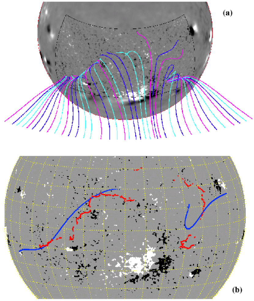
Figure 1.— (a) View from above the ecliptic plane of PFSS field lines traced from the source surface down to the photosphere. Central regions of the high-resolution SOLIS magnetogram are embedded in a lower-resolution synoptic magnetogram for CR 2007. (b) Saturated grayscale version of the high-resolution magnetogram with lines of heliographic longitude and latitude shown at 10° separation (yellow dotted curves). Also shown are footpoint locations of the 8727 high-resolution field lines (red points) and of field lines traced from the same starting locus, but using low-resolution ($\ell_{\rm max}=9$) WSO synoptic data (blue points).

The magnetic polarities in the QS footpoint area of interest were largely mixed and balanced, but there was a slight preponderance of negative polarity in this region of the photosphere. An approximate measurement of the flux imbalance fraction $\xi$ (i.e., the ratio of net flux density to absolute unsigned flux density) yielded $\xi\approx 0.15$, which is well within the range of values expected for QS regions (Wiegelmann & Solanki, 2004; Hagenaar et al., 2008). The slight imbalance toward negative polarities was amplified at larger distances, such that at the PFSS radius the entire 80° wide sector shown in Figure 1(a) was uniformly negative in its polarity. Thus, each of the 8727 open field lines exhibited a negative polarity at their footpoints as well.

If the full set of field lines was mapped down radially from their initial locations to the solar surface, the horizontal separation of each neighboring pair of footpoints would be approximately 110 km. It is clear from Figure 1 that the actual distribution of all 8727 footpoint separations is quite broad. Clumps of closely packed footpoints are separated by wider jumps, the latter occurring in regions where the large-scale polarity changes. The distribution of neighboring footpoint separations spans several orders of magnitude, with minimum, mean, and maximum values of 5.2, 281, and 249,000 km, respectively. The distribution has a median value of 40 km, and it is skewed such that 75% of the neighbor separations are less than 100 km.

In contrast to the statistics of neighboring footpoint separations given above, we note that the SOLIS pixel size is roughly 820 km on the solar surface. Thus, our reconstructed magnetic field lines often tend to oversample the information available in the photospheric data. However, there is evidence that the overlying coronal magnetic field may exhibit topological features—such as nulls, separatrices, and quasi-separatrix layers (QSLs)—that exist on spatial scales smaller than those of the driving sources (e.g., Close et al., 2005b; Antiochos et al., 2007, 2011). It is not clear how much extra resolution is needed in order to resolve these features properly and to produce models that contain the full diversity of flux-tube expansion properties in the open coronal field, so we chose to over-resolve (see also Garraffo et al., 2012).

Figure 2 shows the radial dependence of magnetic field strength along a subset of the high-resolution PFSS field lines. Above the source surface radius of 2.46 $R_{\odot}$, the radial field strength is extrapolated as $B_{r}\propto r^{-2}$. The models described in this section contain no explicit azimuthal field component $B_{\phi}$ above the source surface. At 1 AU, the modeled field strengths range between about $10^{-5}$ and $2.5\times 10^{-5}$ G, which is about a factor of two smaller than is generally measured in the ecliptic (Mariani & Neubauer, 1990). However, the two-dimensional models described in Section 5 contain both a self-consistent Parker spiral field (i.e., $B_{\phi}\neq 0$) and intermittent enhancements of $B_{r}$ due to stream interactions.

For the full set of 8727 modeled field lines, the distribution of field strengths at the photospheric lower boundary has a minimum and maximum of 1.16 and 131 G, respectively. The median photospheric field strength is 24.1 G, the mean is 31.3 G, and the standard deviation about the mean is 26.3 G. Figure 2 shows 36 field lines from the PFSS model: 34 chosen at random, plus the ones with minimum and maximum field strengths at the photosphere. In Figure 2 we also plotted the radial dependence of field strengths for the flux tubes used in the solar wind models of Cranmer et al. (2007).

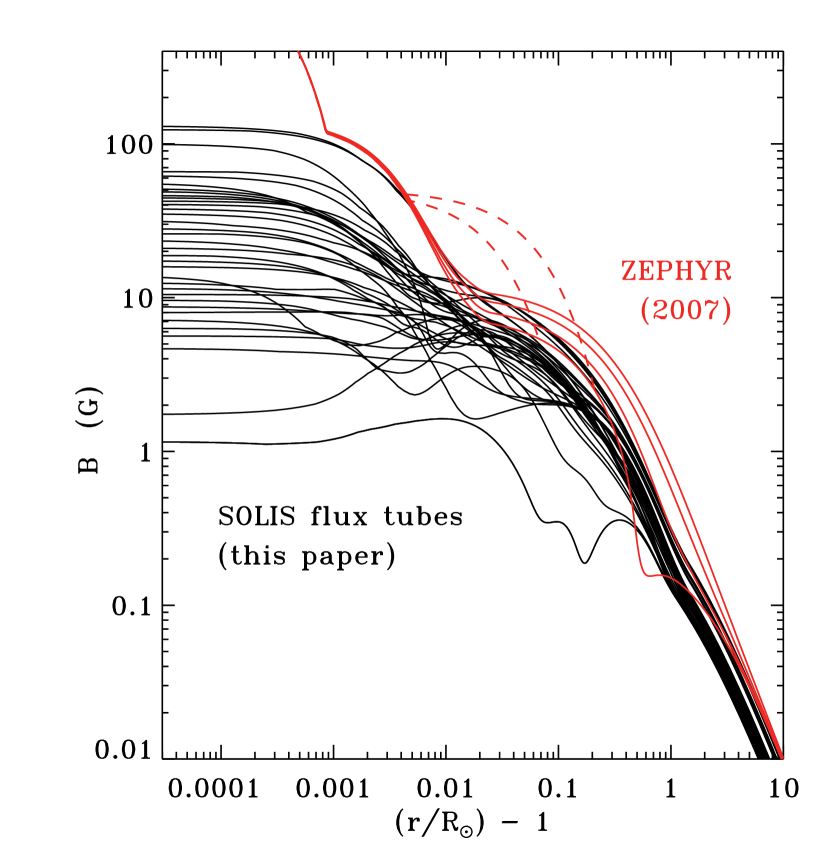
Figure 2.— Radial dependence of magnetic field strengths along a subset of field lines traced in the SOLIS PFSS model (black solid curves). We compare these with the magnetic field distributions used by Cranmer et al. (2007) for ZEPHYR solar wind models. Solid red curves show a range of latitudes in the quiet solar minimum configuration of Banaszkiewicz et al. (1998). Dashed red curves show open flux tubes assumed to be rooted in strong active regions.

We use the modeled radial distributions of field strength to extract a convenient scalar measure of each flux tube’s cross-sectional expansion in the corona. In order to quantify the degree of superradial expansion, we define the Wang-Sheeley-Arge (WSA) expansion factor $f_{\rm ss}$ as

$$f_{\rm ss}\,=\,\frac{(Br^{2})_{\rm base}}{(Br^{2})_{\rm ss}}\,\,,$$ (1)

where the subscript “base” refers to the photospheric lower boundary of the PFSS extrapolation and “ss” refers to the source surface radius of 2.46 $R_{\odot}$. Much like the footpoint locations and photospheric field strengths, we find that $f_{\rm ss}$ varies intermittently with longitude.

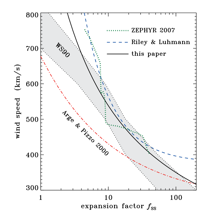
Figure 3.— Empirical relationships between the flux-tube expansion factor $f_{\rm ss}$ and the terminal solar wind speed $u_{\infty}$. Published parameterizations of Arge & Pizzo (2000) (red dot-dashed curve) and Riley & Luhmann (2012) (blue dashed curve) are compared with the original data-ranges given by Wang & Sheeley (1990) (gray region), solar wind model results of Cranmer et al. (2007) (green dotted curve), and Equation (2) (black solid curve).

There are several independent calibrations of the well-known empirical relationship between $f_{\rm ss}$ and the solar wind speed (Wang & Sheeley, 1990; Arge & Pizzo, 2000). These parameterizations depend on the spatial resolution and noise level of the photospheric magnetogram data, as well as on the method used to extrapolate the field (see also Wang et al., 1997; Owens et al., 2005; McGregor et al., 2011; Riley & Luhmann, 2012). Figure 3 compares several of these parameterizations with one another. Note that the Riley & Luhmann (2012) curve largely reproduces the range of values reported by the Wang et al. (1997) revaluation of the original Wang & Sheeley (1990) analysis. Figure 3 also shows a “concordance” WSA relationship that we constructed to fall within the range of the existing correlations. This relationship is given by

$$u_{\infty}\,=\,\frac{2300}{\ln f_{\rm ss}+1.97}\,\,\,\,\,\mbox{km}\,\,\,\mbox{s}^{-1}\,\,,$$ (2)

where $u_{\infty}$ is the terminal or asymptotic solar wind speed. We do not take into account the other commonly used variable parameter of the WSA model: the transverse angular distance $\theta_{b}$ between the field line of interest and the boundary of the nearest large-scale coronal hole. When using this parameter, it is often found that the empirical wind speed becomes independent of this angle for $\theta_{b}\gtrsim{7\arcdeg}$ (e.g., McGregor et al., 2011). The patch of QS in which we model the footpoints of slow solar wind appears to be far enough away from any large coronal holes that these field lines are probably insensitive to $\theta_{b}$.

Figure 4 shows the longitudinal dependence of the flux-tube expansion factor and empirical wind speed $u_{\infty}$ for all 8727 modeled field lines. We also show corresponding parameters of the PFSS model computed from the low-resolution WSO magnetograms. Figure 4(a) plots $f_{\rm ss}$ as a function of a longitudinal angle ($\phi-\phi_{0}$) normalized by the central-meridian Carrington longitude from the high-resolution SOLIS measurement of 2003 September 4. Figure 4(b) shows $u_{\infty}$, computed from Equation (2), as a function of time $t$ estimated for solar wind flux tubes to rotate past the Earth. For this plot, the conversion between longitude and time is given by

$$\phi-\phi_{0}\,=\,-\Omega\left[t-\left(t_{0}+\frac{\Delta r}{\langle u\rangle}\right)\right]\,\,,$$ (3)

where $t_{0}$ is the time that longitude $\phi_{0}$ was on the central meridian, and we use $\Delta r=214\,R_{\odot}$ and $\langle u\rangle=450$ km s^-1 to estimate the mean travel-time from the Sun to 1 AU. Time is plotted in Figure 4 in units of the day of year (DOY) in 2003, and the modeled 80° of longitude converts into approximately 6 days of rotation time. In Figure 4(c) we show a subset of 6 hours to illustrate that extremely sharp structures in $f_{\rm ss}$ exist in the PFSS model that may generate similarly sharp structures in the solar wind (at least close to the Sun). In Section 5 we model the transit-time evolution of the solar wind more accurately.

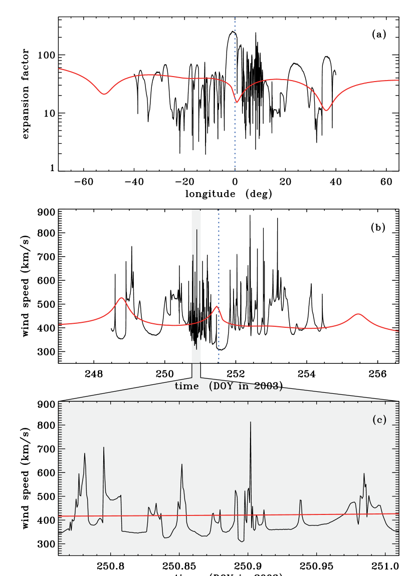
Figure 4.— (a) Longitudinal dependence of $f_{\rm ss}$ computed from the high-resolution SOLIS model (black solid curve) and the low-resolution WSO model (red solid curve). (b) Empirically estimated wind speed $u_{\infty}$ shown as a function of time in day-of-year (DOY) units, with same curve types as in (a). (c) Six-hour expanded subset of the data shown in (b). The central meridian location of the SOLIS high-resolution magnetogram is shown in (a) and (b) with a blue dotted line.

We emphasize that our high-resolution PFSS extrapolation of the Sun’s magnetic field represents merely a single “snapshot” in time. In reality, the small-scale magnetic carpet (Title and Schrijver, 1998) evolves over a wide range of timescales and causes the open-field footpoint locations to move around. Specifically, observations have indicated that the “recycling times” for magnetic flux in the photosphere and corona probably are between 1 and 10 hours (e.g., Close et al., 2005a; Hagenaar et al., 2008). Monte Carlo models of the magnetic carpet’s evolution also found a similar range for the mean timescale of the opening up of closed flux tubes via reconnection (Cranmer & van Ballegooijen, 2010). These times are comparable with how long it takes the radial projection of a supergranular cell to rotate past a distant observer (roughly 3–4 hr). Thus, we do not mean to present the high-resolution PFSS reconstruction as a true dynamical model, but only as a representative state of the QS field that the solar wind will “see” as it accelerates up through the open flux tubes.

3. Non-Potential Radial Enhancements to the Field

The previous section described the straightforward PFSS extrapolation of measured photospheric fields into the corona. However, that process does not take into account the full range of magnetic field variations that we believe exist along these flux tubes. In this section we describe several adjustments that are made to the radial dependence of the magnetic field strength $B(r)$ for the modeled set of time-steady field lines.

First, we recognize that the photospheric footpoints of the large-scale coronal magnetic field appear to be broken up into thin flux tubes (i.e., observed widths of order 50–200 km) that collect in the dark lanes between the $\sim$1000 km diameter granulation cells. These flux tubes have field strengths of 1–2 kG and are often called “G-band bright points” (GBPs) because they show up as bright features in the 4290–4320 Å molecular bands (e.g., Berger et al., 1995; Steiner et al., 2001). Horizontal motions of these features have been used to put empirical constraints on the photospheric flux of Alfvén wave energy that propagates up into the corona (Nisenson et al., 2003; Cranmer & van Ballegooijen, 2005; Chitta et al., 2012). GBPs do not show up individually in the SOLIS magnetograms that we used to reconstruct the coronal field, so we modify $B(r)$ as described below to account for their supposed presence.

Figure 5(a) illustrates how the assumption of photospheric field fragmentation results in narrower flux tubes and higher field strengths than would be otherwise obtained from the magnetogram data. Somewhat crudely, we assume the lower solar atmosphere is divided into strong-field flux tubes and “field free” regions that are in total pressure equilibrium with one another. Enhancing the field strength inside the flux tube is equivalent to assuming a larger field-free volume between the tubes. Thus, along each flux tube we modify the original PFSS field $B_{\rm 0}(r)$ by adding two additional components in quadrature; i.e.,

$$B^{2}\,=\,B_{0}^{2}+B_{1}^{2}+B_{2}^{2}\,\,\,.$$ (4)

The photospheric GBP enhancement $B_{1}$ is given by

$$B_{1}(z)\,=\,B_{\odot}\,\exp\left(-\frac{z}{2H_{1}}\right)\,\,,$$ (5)

where $z=r-R_{\odot}$ is the height above the (optical depth unity) photosphere, and we adopt $B_{\odot}=1470$ G as a universal GBP field strength. The upper photospheric scale height $H_{1}=120$ km corresponds to a hydrostatic temperature of approximately 4000 K. These constants result in a field strength that matches the photospheric and lower chromospheric parts of the Cranmer & van Ballegooijen (2005) flux tube model.

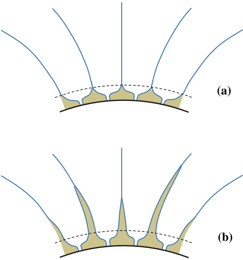
Figure 5.— Schematic illustration of flux-tube expansion in the presence of non-potential fields. In both panels, open flux tube boundaries (blue solid curves) surround empirically determined field-free regions (gold areas). (a) For $B_{1}\neq 0$ and $B_{2}=0$, the only enhancements to the open field occur below the mid-chromospheric “merging height” (dashed curve) of Cranmer & van Ballegooijen (2005). (b) Postulated field enhancements in both the photosphere and the low corona are shown (i.e., $B_{1}\neq 0$ and $B_{2}\neq 0$).

There is evidence that additional modifications to a potential field (i.e., the $B_{2}$ term above) are needed in the corona. For example, Cranmer & van Ballegooijen (2005) took account of the large-scale bundling of fields in the supergranular network of a coronal hole by constructing a two-dimensional magnetostatic model of the canopy-like expansion of open flux tubes (see also Gabriel, 1976; Giovanelli, 1980; Hackenberg et al., 2000; Aiouaz & Rast, 2006). The presence of weak-field regions in the internetwork cell centers (with presumably higher gas pressure than the strong-field network lanes) modifies the potential field expansion at chromospheric heights. Similarly, Schrijver & van Ballegooijen (2005) studied the modifications to a potential field due to the presence of finite gas pressure gradients throughout the low corona. They modeled the spatial dependence of the plasma $\beta$ parameter (i.e., the ratio of gas pressure to magnetic pressure) in a QS region and found that $\beta\approx 1$ over much of the volume. This implies the gas influences the field topology in ways unanticipated by the potential field model, which implicitly assumes $\beta\ll 1$.

It is well known that active regions frequently contain large-scale currents that give rise to twisted, sigmoidal field lines (e.g., Gary et al., 1987; Canfield et al., 1999; Schrijver et al., 2005). These structures are believed to be the result of a combination of surface shear motions and the emergence of new flux from below the solar surface. However, because these effects also occur elsewhere on the Sun, it is likely that other regions (including the QS footpoints of open flux tubes) exhibit currents and non-potential fields on a wide range of spatial scales (see Abbett, 2007; Zhao et al., 2009; Yeates et al., 2010; Reardon et al., 2011; Meyer et al., 2012). These effects give rise to increased “fibril” type complexity to the field. Their presence is likely to increase the field strength in the low corona and thus shrink the volume of any given open flux tube that traverses the non-potential region (see Figure 5(b)). Other physical effects that may contribute to modifying the radial dependence of $B$ include pervasive chromospheric upflows (McIntosh & De Pontieu, 2009), rotational supergranule motions (Zhang & Liu, 2011), and loop footpoint asymmetries that give rise to rapid unresolved motions (Wiegelmann et al., 2010).

In the absence of a clear-cut method of modeling non-potential field enhancements in the low corona, we adopt a similar hydrostatic radial dependence as was used in Equation (5). The added magnetic field component is given by

$$B_{2}(z)\,=\,B_{0}(0)\,\exp\left(-\frac{z}{2H_{2}}\right)\,\,,$$ (6)

where an approximate scale height $H_{2}=2k_{\rm B}T_{2}/(m_{p}g)$ is defined by an arbitrary effective temperature $T_{2}$, the Boltzmann constant $k_{\rm B}$, the proton mass $m_{p}$, and the Sun’s surface gravitational acceleration $g$. Because the primary goal of this non-potential enhancement is to “stretch out” the pre-existing field, it is normalized using the PFSS lower boundary condition $B_{0}(0)$ of that particular field line. The effective temperature $T_{2}$ is a purely empirical parameter that characterizes the radial extent of the $B_{2}$ field modification. The only way that $T_{2}$ would be related to an actual coronal temperature would be if gas pressure effects were the primary cause of the non-potential enhancement (see, e.g., Schrijver & van Ballegooijen, 2005).

Figure 6(a) illustrates the magnetic field enhancements described above using a mean PFSS model. The unmodified field strength $B_{0}$, shown by the dashed curve, was produced by forming the average of $\ln B_{0}$ at each height and taking the exponential of the result. The photospheric enhancement $B_{1}$ dominates the modified field strength at heights $z\lesssim 0.002\,R_{\odot}$. The other curves show the result of varying the effective scale-height temperature $T_{2}$ in Equation (6). Values of $T_{2}$ between about 0.05 and 0.5 MK represent mild enhancements to the field strength in the low corona that are consistent with the flux-tube constrictions illustrated in Figure 5(b). The red curve corresponding to the largest field strength in Figure 6, which was computed for $T_{2}=1.5$ MK, is probably beyond the realm of physical realism. Generally, we do not expect the non-potential effects described above to extend as far up as $z\gtrsim 0.5\,R_{\odot}$ in a QS region. We also do not believe that using a value of $T_{2}$ that is of the same order of magnitude as the expected peak coronal temperature is especially realistic, either. We show the $T_{2}=1.5$ MK curve mainly for the sake of completeness.

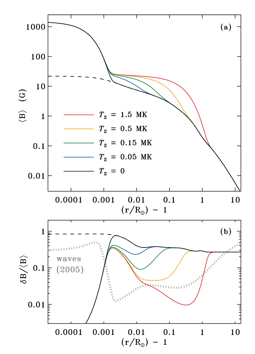
Figure 6.— Radial dependence of (a) mean magnetic field strengths and (b) ratios of rms field strength fluctuations to the mean field strengths. The unmodified $B_{0}$ model (black dashed curve) is shown with a model that includes only the $B_{1}$ enhancement (black solid curve) and others that also contain the $B_{2}$ coronal enhancement (color solid curves, see labels for $T_{2}$ values). Also shown in (b) is the ratio of rms to mean field strength in the non-WKB Alfvén wave model of Cranmer & van Ballegooijen (2005) (gray dotted curve).

In Figure 6(b) we show a measure of the statistical variability of the field strength in the whole set of 8727 SOLIS flux tubes. The plotted quantity is the ratio of the standard deviation in $B$ to its mean value at a given height. As above, the dashed line shows the unmodified field strength $B_{0}$, which reaches a maximum ratio of $\sim$0.84 in the photosphere and declines to about 0.27 at the source surface. When the $B_{1}$ and $B_{2}$ enhancements are added there is necessarily a smaller degree of variability in $B$, especially for the strong photospheric component at low heights. In the corona, the ratio gets smaller for two reasons of nearly comparable magnitude to one another: (1) the mean field strength increases, and (2) the standard deviation decreases. We also compare these ratios of relative variability to a representative model of Alfvén wave variability from Cranmer & van Ballegooijen (2005). The plotted quantity is the ratio of the root mean squared (rms) Alfvénic fluctuation amplitude $\delta B$ to the background field strength $B_{0}$. Of course, this is somewhat an “apples to oranges” comparison because the Alfvénic variability represents propagating transverse waves and the other curves describe a collection of static spatial fluctuations. Nonetheless the overall similarity of the two ratios indicates that the two types of variations may be of comparable importance in the low corona.

We chose not to include the non-potential field enhancements $B_{1}$ and $B_{2}$ in our calculations of the superradial expansion factor $f_{\rm ss}$ for each field line. These enhancements are included mainly for the benefit of the ZEPHYR simulations, which make use of the Alfvén speed profile in the lower atmosphere to translate photospheric velocity amplitudes into wave energy fluxes. If we had inserted the modified field strengths in Equation (1) to rescale $f_{\rm ss}$, the basal field strengths would all be nearly identical to one another due to the $B_{1}$ term. In that case, much of the relevant information about field-line spreading in the upper chromosphere and low corona (which is contained in the measured variability of $B_{0}(0)$) would have been erased from $f_{\rm ss}$.

4. Turbulence-Driven Solar Wind Models

We used the computed magnetic fields $B(r)$ as inputs to a series of one-dimensional physical models of turbulent coronal heating and solar wind acceleration. The steady-state models presented below are numerical solutions to one-fluid conservation equations for mass, momentum, bulk internal energy, and Alfvén wave energy. Cranmer et al. (2007) described these equations and outlined the computational methods used to solve them using a computer code called ZEPHYR. The models presented below were calculated with a slightly modified version of the original ZEPHYR code. In addition to several algorithmic improvements that were needed to allow the code to read in large numbers of flux tubes at a time, we made three modifications that affected the results:

1. We changed the value of the coefficient that multiplies Hollweg’s (1974, 1976) prescription for free-streaming conductive heat flux in the collisionless heliosphere. Cranmer et al. (2007) used $\alpha_{c}=4$, as originally suggested by Hollweg, but we reduced it to $\alpha_{c}=1$ based on a recent analysis of electron heat flux measurements in the fast solar wind (see Cranmer et al., 2009).

2. We reduced the photospheric boundary condition on the energy flux of longitudinal acoustic waves from $10^{8}$ to $10^{6}$ erg s^-1 cm^-2. The lower value gave a more realistic height for the transition region (TR) between the chromosphere and corona than did the higher value. Figure 8 of Cranmer et al. (2007) showed that a larger acoustic wave pressure in the chromosphere gives rise to a larger density scale height and thus causes the “critical” density for runaway radiative instability to occur at a larger height. Our adopted value of the acoustic wave flux, in combination with the Cranmer et al. (2007) choice for the photospheric Alfvén wave amplitude ($v_{\perp}=0.255$ km s^-1), was held fixed for all of the models discussed below.

3. We used the modified version of the numerical relaxation method for the internal energy equation described by Cranmer (2008). We also reduced the initial value of the minimum undercorrection exponent $\epsilon_{0}$ from 0.17 to 0.10. These changes gave rise to more robust convergence of the coronal and heliospheric temperature $T(r)$ to its steady-state solution.

It should also be emphasized that ZEPHYR code makes use of the full radial dependence of $B(r)$ and does not depend on the spatial resolution of observations that can affect the normalization of the expansion factor $f_{\rm ss}$.

Prior to computing models for a large number of flux tubes from the SOLIS reconstruction, we performed a limited parameter study to explore the effects of varying the non-potential field enhancement $B_{2}$. We began with the mean-field models shown in Figure 6(a) and produced a finer grid that varied the $T_{2}$ parameter from 0 to 1.5 MK in increments of 0.025 MK. These models all used identical lower boundary conditions in the photosphere, and only differed in their tabulated $B(r)$ field strengths. Of those 61 models, 52 of them converged successfully to a steady-state solution that satisfied internal energy conservation to within 5% accuracy. The other 9 models corresponded to values of $T_{2}>0.9$ MK, which we suspect is outside the realm of physical realism for the non-potential field enhancements.

In Figure 7 we show several summary parameters of the successful subset of mean-field ZEPHYR models that varied the $T_{2}$ parameter. As the non-potential field strength in the low corona is increased, the wind speed $u$ at 1 AU decreases and the proton number density $n_{p}$ at 1 AU increases. Figure 7(a) shows that most of this variation occurs as $T_{2}$ is increased from 0 to 0.5 MK. Subsequent increases from 0.5 to 1.5 MK do not appear to produce substantial changes in the modeled solar wind. Figure 7(b) plots the maximum coronal temperature versus the Alfvén wave velocity amplitude $v_{\perp}$ at 1 AU. One can think of this value of $v_{\perp}$ as a “residual” amplitude since it is the end result of wave dissipation that occurred in the corona and inner heliosphere. It makes sense that larger coronal temperatures correspond to smaller values of $v_{\perp}$, since more coronal heating is consistent with more damping of MHD turbulence.

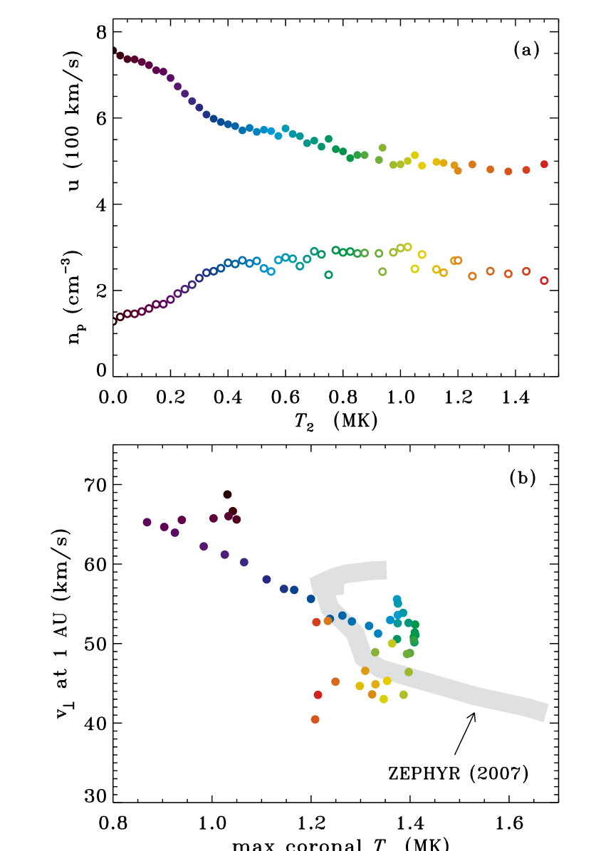
Figure 7.— Results of mean-field ZEPHYR solar wind models for a range of $T_{2}$ parameters. (a) Wind speed at 1 AU in units of 100 km s^-1 (solid symbols) and proton number density at 1 AU (open symbols). Symbol colors are mapped directly to the $T_{2}$ values shown on the horizontal axis. (b) Alfvén wave velocity amplitude at 1 AU plotted vs.  the peak coronal temperature for the mean-field models (symbols with same $T_{2}$ colors as in panel (a)) and for the models presented by Cranmer et al. (2007) (gray region).

We can explain the variations shown in Figure 7 by noticing that the turbulent heating rate $Q$ is often close to being linearly proportional to the background field strength $B$ in the upper chromosphere and low corona. Cranmer (2009) showed that this proportionality is exact in cases where both the thin flux-tube relation ($B\propto\rho^{1/2}$) and sub-Alfvénic wave action conservation ($v_{\perp}\propto\rho^{-1/4}$) are valid. Thus, when the field strength $B_{2}$ is increased, the amount of heat deposited at the coronal base increases as well. In direct response, the corona’s base pressure increases, as does the solar wind’s mass loss rate (see Hammer, 1982; Withbroe, 1988; Cranmer & Saar, 2011). This explains why the peak coronal temperature and the proton number density at 1 AU both increase when $T_{2}$ is increased. The decrease in $v_{\perp}$ at 1 AU was explained above as a result of the increased wave damping that goes along with stronger coronal heating.

The variation in the wind speed $u$ in Figure 7 can be understood as a result of the presence of ponderomotive wave-pressure acceleration (Jacques, 1977; Holzer et al., 1983). When the relative strength of coronal heating is low (i.e., for the smallest values of $T_{2}$), the wind is driven primarily by wave pressure and not gas pressure. In that regime, there is a higher outflow speed when there is a stronger (less damped) population of Alfvén waves both in the corona and at 1 AU. Figure 7(b) shows that when $T_{2}$ is smaller than about 0.25 MK, the corona is heated to peak temperatures below 1 MK and the residual wave amplitude at 1 AU is higher than was seen in the Cranmer et al. (2007) ZEPHYR models. Thus, we may be able to rule out values of $T_{2}$ below $\sim$0.25 MK because of their unrealistic solar wind properties. If we combine this with the discussion above that appeared to also rule out values of $T_{2}$ larger than 1–1.5 MK, this leaves only a limited range of $T_{2}$ parameters (i.e., $0.25\lesssim T_{2}\lesssim 0.75$ MK) that may be relevant for modeling our reconstructed QS flux tubes.

With the above results in mind, we proceeded to create solar wind models for the SOLIS flux tubes discussed in Section 2. Because the full set of 8727 flux tubes often oversamples the existing complexity of the reconstructed magnetic field, we selected a subset of 289 field lines to input to ZEPHYR. These field lines were chosen by sampling the data more frequently in regions of rapid longitudinal change than in regions where the field strength was nearly constant. Every local maximum and minimum in the longitudinal variation of $f_{\rm ss}$ (see Figure 4(a)) was represented by at least one of the 289 resampled points. We ran ZEPHYR for three distinct cases of non-potential field enhancement: (1) $T_{2}=0$ (i.e., using the photospheric $B_{1}$ enhancement only), (2) $T_{2}=0.2$ MK, and (3) $T_{2}=0.5$ MK. We decided against using even larger values of $T_{2}$ because Figure 7 showed that the resulting solar wind would probably not have been significantly different from the $T_{2}=0.5$ MK case.

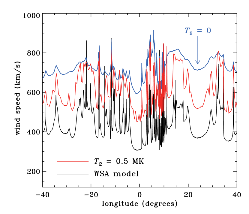
Figure 8.— Comparison of asymptotic solar wind speeds estimated from the WSA anticorrelation (lower black curve) with those computed from ZEPHYR models having $T_{2}=0$ (upper blue curve) and $T_{2}=0.5$ MK (middle red curve). Longitudes are plotted for the footpoints of the PFSS flux tubes as in Figure 4(a).

Figure 8 summarizes the results of two of the ZEPHYR models ($T_{2}=0$, 0.5 MK) by comparing the wind speeds at 1 AU with the predicted WSA wind speed from Equation (2). The intermediate case of $T_{2}=0.2$ MK exhibits plasma properties that lie between the two plotted models. Note that an overall WSA-type anticorrelation between $u$ and $f_{\rm ss}$ appears to be upheld for the numerical models. As was discussed above, the $T_{2}=0$ models do not contain enough turbulent heating to give rise to coronal temperature maxima above 1 MK. Thus, the resulting lack of wave dissipation gives rise to “too much” wave pressure acceleration and a high-speed, low-density wind. The case of $T_{2}=0.5$ MK gives rise to wind speeds at 1 AU between 448 and 853 km s^-1, which is a bit higher than the observed range of speeds but is much more realistic than the predictions of the $T_{2}=0$ model.

In Figure 9(a) we examine in more detail how the models appear to follow WSA-like relationships between wind speed and expansion factor. Although there is substantial scatter, each set of ZEPHYR results does seem to be centered around a relationship reminiscent of Equation (2). Models with lower values of $T_{2}$ correspond to larger normalization offsets in the wind speed. For the $T_{2}=0.5$ MK case, we show the modeled wind speeds measured at a heliospheric distance of $r=20\,R_{\odot}$ in addition to those at 1 AU. At the former distance the wind speed in each flux tube is roughly 75% of its asymptotic terminal speed in interplanetary space. Those speeds agree remarkably well with the curve corresponding to Equation (2). This is consistent with the fact that the empirical WSA relationship is often applied as a lower boundary condition (typically at distances of order 20 $R_{\odot}$) for global simulations of the inner heliosphere (e.g., Lee et al., 2009; McGregor et al., 2011).

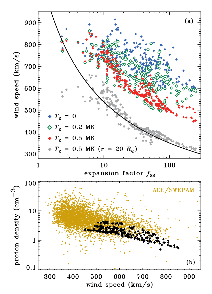
Figure 9.— (a) Solar wind speeds plotted vs.  $f_{\rm ss}$ compared with Equation (2) (black solid curve). Speeds at 1 AU are shown for ZEPHYR models having $T_{2}=0$ (blue filled symbols), $T_{2}=0.2$ MK (green open symbols), and $T_{2}=0.5$ MK (red filled symbols). Speeds at $r=20\,R_{\odot}$ are also shown for the $T_{2}=0.5$ MK model (gray filled symbols). (b) Proton number densities $n_{p}$ at 1 AU plotted vs.  wind speeds for the $T_{2}=0.5$ MK model (large black symbols) and for ACE/SWEPAM data (small gold symbols).

It is difficult to pin down a simple explanation for the emergence of clear WSA anticorrelations in Figure 9(a). There have been various attempts to explain how an Alfvén wave driven wind should exhibit this kind of relationship between wind speed and expansion factor (Kovalenko, 1981; Wang & Sheeley, 1991; Suzuki, 2006). These explanations tend to involve differences in the radial evolution of wave energy flux along different field lines—i.e., larger wave fluxes at the critical point correspond to both greater acceleration and smaller values of $f_{\rm ss}$. This must be happening to some extent, but the ZEPHYR models also include non-WKB reflection, self-consistent wave damping, and wind acceleration from both gas pressure and wave pressure. These effects are linked to one another via a number of nonlinear feedbacks, so we do not yet know the precise chain of events that gives rise to the emergent distribution of wind speeds. Future work (e.g., Woolsey & Cranmer, 2012) will aim to determine whether these interactions can be understood from the standpoint of more basic scaling relations.

Figure 9(b) shows the anticorrelation between wind speed and proton number density at 1 AU. In addition to the $T_{2}=0.5$ MK model results, we also show hourly-averaged data measured by the Solar Wind Electron, Proton, and Alpha Monitor (SWEPAM) instrument on the Advanced Composition Explorer (ACE) spacecraft (McComas et al., 1998). The data displayed are a relatively sparse selection of approximately 4700 data points spread out in time between the years 1998 and 2006. Even though the models do not extend to the lowest wind speeds and highest densities seen in the low-latitude heliosphere, the overall sense of agreement between the models and the measurements is good.

To illustrate the plasma properties that appear in the ZEPHYR models, we show in Figure 10 the temperatures, outflow speeds, and magnetic field strengths for a selection of five flux tubes from the $T_{2}=0.5$ MK model. In the low corona, the magnetic field strengths in these flux tubes vary over about an an order of magnitude (from 4 to 40 G). However, Figure 10(c) shows that $B(r)$ does not vary substantially in the photosphere and chromosphere ($z\lesssim 0.002\,R_{\odot}$) nor in the extended corona and heliosphere ($z\gtrsim 0.5\,R_{\odot}$) of these models. As described above, stronger coronal fields give rise to more heating below the critical point, which in turn produces a hotter, denser, and ultimately slower wind (see also Leer & Holzer, 1980; Pneuman, 1980; Leer et al., 1982). Figure 10(b) shows that the hotter models undergo more intense “bursts” of solar wind acceleration in the low corona, but their large-scale outflows end up being slower.

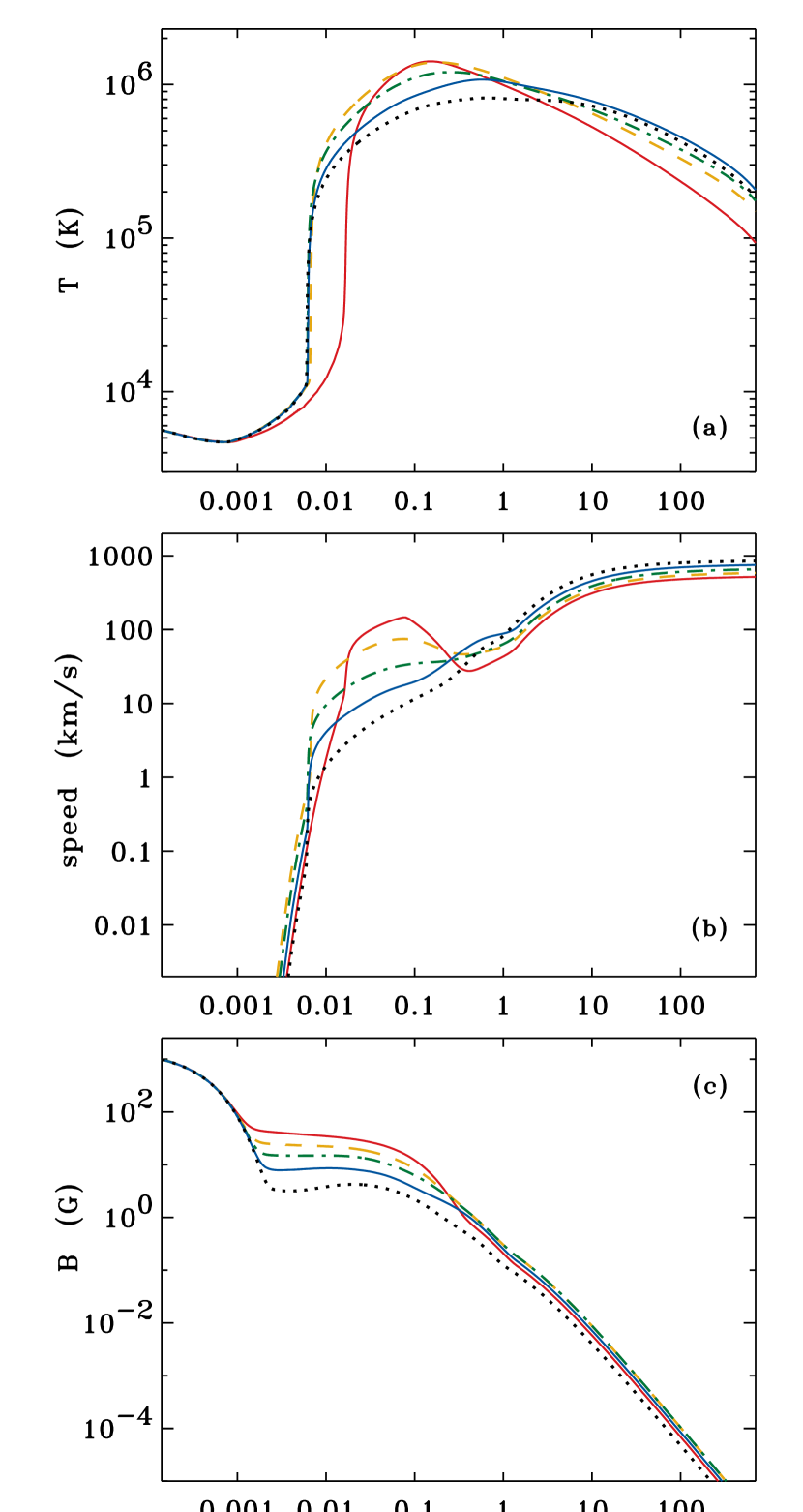
Figure 10.— Radial dependence of solar wind parameters for a selection of five flux tubes extracted from the ZEPHYR models computed with $T_{2}=0.5$ MK. Shown are: (a) one-fluid temperatures, (b) radial wind speeds, and (c) magnetic field strengths vs.  height above the solar photosphere. Line styles and colors serve merely as consistent identifying labels for the flux tubes.

Figure 10(a) shows that the model receiving the largest degree of coronal heating has a higher TR than the other models. This occurs because that model’s intense wave pressure in the upper chromosphere produces a larger pressure scale height and a shallower radial decline in the density. Thus, the density does not drop to its critical value (for runaway radiative instability) until it reaches a significantly larger height than in the other models. A situation similar to the above case occurs for roughly half of the full set of 289 ZEPHYR models computed with $T_{2}=0.5$ MK. Defining the TR height $z_{\rm TR}$ as the location at which $T$ first exceeds 0.2 MK, we found that the models bifurcate cleanly into two groups: 162 of them had $z_{\rm TR}\leq 0.008\,R_{\odot}$ and 127 of them had $z_{\rm TR}\geq 0.012\,R_{\odot}$. As expected, the latter set of models with larger values of $z_{\rm TR}$ tended to have larger peak temperatures ($T_{\rm max}\gtrsim 1.3$ MK) and lower asymptotic wind speeds ($u_{\infty}\lesssim 600$ km s^-1) than the other models. This appears to be a kind of “bistable” situation, and it is possible that a truly time-dependent model would exhibit oscillations between these two states. We will study this effect in future work.

5. Interplanetary Evolution of the Solar Wind

Each of the individual ZEPHYR models described above was computed independently of the others. However, we know that magnetic flux tubes in the corona and heliosphere interact with their “neighbors” in a variety of ways. The distinct identity of a given flux tube can be blurred by time-dependent disruptive effects such as Kelvin-Helmholtz instabilities (e.g., Einaudi et al., 1999; Parhi et al., 1999; Velli et al., 2011) or diffusive field-line shredding due to MHD turbulence (Mullan, 1991; Matthaeus et al., 1995). Also, the large-scale structure of the heliosphere is often dominated by collisions between obliquely oriented streams that result in CIR-like compressions and rarefactions.

Our goal in this section is to begin taking account of the multidimensional evolution of solar wind flux tubes as initially computed from the high-resolution magnetic field models of Sections 2–4. We use the longitudinally resolved set of ZEPHYR plasma properties as an inner boundary condition to a two-dimensional MHD calculation in the ecliptic plane. Thus, we simulate the time-steady effects of CIR formation, but we do not yet include any smaller scale time-dependent effects (e.g., waves, instabilities, or turbulence) on the interplanetary evolution of these flux tubes.

For a frame corotating with constant angular velocity $\Omega$, Whang (1980) and Hu (1993) described the time-steady MHD conservation equations in the ecliptic plane ($\theta=\pi/2$). In general, we solve for the six magnetofluid parameters $\rho$ (mass density), $v_{r}$ (radial velocity), $v_{\phi}$ (azimuthal velocity), $P$ (gas pressure), $B_{r}$ (radial field strength), and $B_{\phi}$ (azimuthal field strength) as a function of $r$ and $\phi$. Mass conservation is given by

$$\frac{1}{r^{2}}\frac{\partial}{\partial r}\left(r^{2}\rho v_{r}\right)+\frac{1}{r}\frac{\partial}{\partial\phi}\left(\rho v_{\phi}\right)\,=\,0\,\,.$$ (7)

The two nontrivial components of momentum conservation are

$$v_{r}\frac{\partial v_{r}}{\partial r}+\frac{v_{\phi}}{r}\frac{\partial v_{r}}{\partial\phi}+\frac{1}{\rho}\frac{\partial P}{\partial r}+\frac{GM_{\odot}}{r^{2}}\,\,\,=$$

$$\frac{B_{\phi}}{4\pi\rho}(\nabla\times{\bf B})_{\theta}+\frac{v_{\phi}^{2}}{r}+\Omega(2v_{\phi}+\Omega r)$$ (8)

$$v_{r}\frac{\partial v_{\phi}}{\partial r}+\frac{v_{\phi}}{r}\frac{\partial v_{\phi}}{\partial\phi}+\frac{1}{\rho r}\frac{\partial P}{\partial\phi}=-\frac{B_{r}}{4\pi\rho}(\nabla\times{\bf B})_{\theta}-\frac{v_{r}v_{\phi}}{r}-2\Omega v_{r}$$ (9)

where $G$ is the Newtonian gravitation constant, $M_{\odot}$ is the solar mass, and the latitudinal component of the curl of ${\bf B}$ is given by

$$(\nabla\times{\bf B})_{\theta}\,=\,\frac{1}{r}\frac{\partial B_{r}}{\partial\phi}-\frac{\partial B_{\phi}}{\partial r}-\frac{B_{\phi}}{r}\,\,.$$ (10)

The internal energy equation for pressure is

$$v_{r}\frac{\partial P}{\partial r}+\frac{v_{\phi}}{r}\frac{\partial P}{\partial\phi}+\rho a^{2}\left[\frac{1}{r^{2}}\frac{\partial}{\partial r}\left(r^{2}v_{r}\right)+\frac{1}{r}\frac{\partial v_{\phi}}{\partial\phi}\right]\,=\,0\,\,,$$ (11)

and the equation of state $\gamma P=\rho a^{2}$ defines the single-fluid sound speed $a$. We choose a constant value for the adiabatic exponent $\gamma$. The divergence-free constraint on the magnetic field gives rise to an effective conservation equation for $B_{r}$, which is

$$\frac{1}{r^{2}}\frac{\partial}{\partial r}\left(r^{2}B_{r}\right)+\frac{1}{r}\frac{\partial B_{\phi}}{\partial\phi}\,=\,0\,\,.$$ (12)

Lastly, the “frozen-in” MHD assumption that the magnetic field vector remains parallel to the corotating velocity vector allows us to write $B_{\phi}=v_{\phi}B_{r}/v_{r}$. Making use of the defining equations for $a$ and $B_{\phi}$ leaves 5 equations for 5 unknowns ($\rho$, $v_{r}$, $v_{\phi}$, $P$, $B_{r}$).

The MHD equations as described above involve a number of key approximations. Our neglect of explicit time dependence results in the elimination of MHD waves from the modeled system. However, these equations do contain the terms needed to model information propagation on MHD characteristics, which was used by Hu (1993) to successfully predict the formation of shocks in the outer heliosphere. Note that we also neglect the source terms in the momentum and internal energy equations that were required to produce turbulent coronal heating and wave-pressure acceleration in the ZEPHYR models. Thus, we are essentially replacing the effects of turbulent heating at heights above our inner boundary radius (i.e., $r>20\,R_{\odot}$) with a simple gas pressure gradient determined by the adopted value of the polytropic exponent $\gamma$.

To solve Equations (7)–(12), we first constructed the $5\times 5$ matrices that contain the coefficients multiplying the $r$ and $\phi$ partial derivatives. Following Hu (1993), we inverted the first of those matrices and solved for each of the $r$ derivatives by themselves. To step upward from a lower boundary radius, we implemented the first-order upwind differencing technique described by Press et al. (1992) and Riley & Lionello (2011). The approach of Riley & Lionello (2011) was to solve an inviscid Burgers’ equation that corresponds to Equation (8) in the limit of $a\rightarrow 0$ and $V_{\rm A}\rightarrow 0$. We extended their upwind differencing technique to the full set of corotating MHD equations, and we used the standard Courant-Friedrichs-Lewy (CFL) criterion (treating $r$ as the time-like variable and $\phi$ as the space-like variable) to set the radial step size.

To test our numerical implementation of the MHD equations, we solved the example problem of a single “trapezoidal” shaped high-speed stream that was posed by Hu (1993). Starting at a lower boundary radius of 0.3 AU, the wind speed was doubled (from 300 to 600 km s^-1) in a 60° wide band of longitude, the density was correspondingly reduced such that $\rho\propto v_{r}^{-1.5}$, and the gas pressure was assumed to remain constant. This model used an ideal adiabatic value of $\gamma=5/3$. Figure 11 shows the results of evolving these conditions from 0.3 to 1 AU, and it compares favorably to the properties shown in Figure 8 of Hu (1993). Instead of plotting the azimuthal velocity $v_{\phi}$ in the corotating frame, Figure 11(b) shows the azimuthal velocity in the inertial frame,

$$u_{\phi}\,=\,v_{\phi}+\Omega r\,\,,$$ (13)

which exhibits departures from zero only because of the stream-stream interactions that grow in magnitude with increasing heliocentric distance.

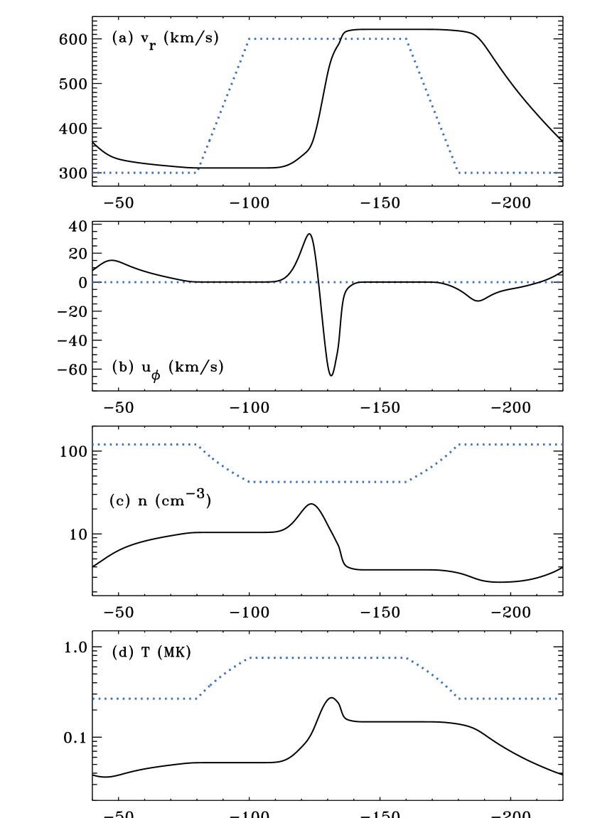
Figure 11.— Azimuthal profiles of plasma properties computed for the Hu (1993) test problem and shown at $r=0.3$ AU (blue dotted curves) and $r=1$ AU (black solid curves). Shown are: (a) radial wind speed $v_{r}$, (b) azimuthal speed in the inertial frame $u_{\phi}$, (c) proton number density $n=\rho/m_{p}$, and (c) one-fluid temperature $T$. The azimuthal angle $\phi$ has been shifted by a constant offset to have the scale line up with that of Figure 8 of Hu (1993).

Next, we made use of the ZEPHYR solar wind models as inner boundary conditions for a two-dimensional model of the heliosphere in the ecliptic plane. We focused only on the standard parameter choice of $T_{2}=0.5$ MK that was used for the models shown in Figure 10. We extracted the density, wind speed, gas pressure, and magnetic field strength as a function of $\phi$ at an inner boundary radius chosen initially to be $r=20\,R_{\odot}$. We chose to set $v_{\phi}=-\Omega r$ at this radius, which is equivalent to assuming no rotation in the inertial frame ($u_{\phi}=0$) as is appropriate for a height well above the solar wind’s Alfvén point (see, e.g., Weber & Davis, 1967). Although we assume time-steady corotation of MHD “patterns” in this model system, that is not equivalent to the rigid rotation of the fluid itself (i.e., assuming $v_{\phi}=0$ would be unrealistic).

The fully resolved SOLIS flux tubes subtend only 80° out of a full 360°, so we interpolated the plasma parameters linearly throughout the unused 280° of longitude. We used a fine azimuthal grid with 39279 zones and constant separation $\Delta\phi=0.00917\arcdeg$. We set $\gamma=1.2$ to account for ongoing gradual heating in the range of distances to be modeled in the ecliptic plane. This exponent is roughly consistent with an in situ temperature dependence of roughly $T\propto r^{-1/2}$, which is close to what is seen for the average of proton and electron temperatures in the inner heliosphere (e.g., Cranmer et al., 2009).

When running the two-dimensional MHD code for the high-resolution set of SOLIS flux tubes, we found that in some cases the standard CFL criterion did not govern the numerical stability of the upwind differencing scheme. In these cases, even the use of a radial step size several orders of magnitude smaller than dictated by CFL would not stabilize the system’s evolution. We found that Equation (9), the azimuthal momentum conservation equation, was responsible for this instability. Although Hu (1993) found that standard MHD characteristics are valid for these equations in the supersonic and super-Alfvénic limits, it is possible that the Coriolis and curvature terms in Equations (8)–(9) modify the system’s effective “wave speeds” such that the smaller azimuthal flows require special treatment. In practice, we found two alternate ways of producing stable models:

1. One solution was to assume that deviations from strict “Parker spiral” corotation (i.e., $v_{\phi}=-\Omega r$) can be neglected. Figure 11(b) showed that departures from $u_{\phi}=0$ at large-scale stream interfaces are typically subsonic in magnitude and thus probably unimportant to the overall dynamics of CIRs. By making the assumption that $v_{\phi}$ has a known analytic value, we were able to exclude Equation (9) from the system of equations solved by the code. The strict upwind differencing method suggested by Riley & Lionello (2011) remained stable for CFL-compliant radial step sizes. We refer to this as our “low-diffusion” model.

2. Another solution was to solve the $v_{\phi}$ equation using a method that was both more numerically stable and more diffusive. We applied the Lax method (see, e.g., Press et al., 1992) to the solution of Equation (9), but we kept the less diffusive upwind differencing method for the other four MHD equations. The inclusion of departures from strict corotation (i.e., allowing the system to develop longitudinal variations in $v_{\phi}$) also gives rise to additional physical diffusion in $\phi$. Both types of diffusion contribute to the smearing out of sharp structures in longitude. Thus, we refer to this case as our “high-diffusion” model.

Below we show results from both models. We believe the true solutions to Equations (7)–(12) should lie in between the results of the low and high diffusion cases.

Figure 12 shows how the longitudinal profile of radial velocity $v_{r}$ evolves with increasing radial distance. The “leftward” evolution of structures in $\phi$ is due to the curvature of the overall Parker spiral. As predicted by Wang & Sheeley (2003) and others, the strongest and narrowest velocity peaks at the inner boundary are rapidly smeared out by interactions with surrounding slow wind. At the intermediate distance of 40 $R_{\odot}$ shown in Figure 12(b), the high-diffusion model looks somewhat like a smoothed version of the low-diffusion model. However, by the time the streams reach 1 AU (Figure 12(c)), there has been enough dynamical evolution to make the two models appear quite different from one another.

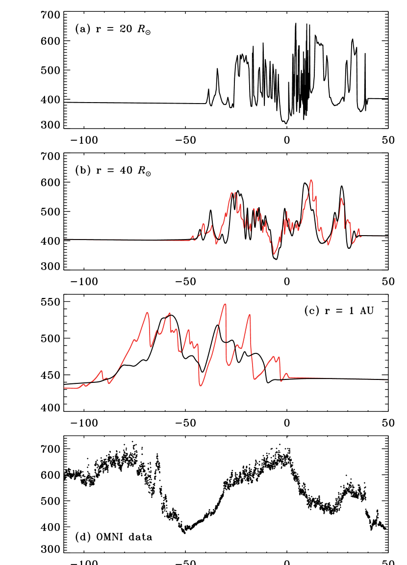
Figure 12.— Radial wind speeds for MHD models computed from ZEPHYR solar wind properties. (a) The inner boundary radius $r=20\,R_{\odot}$ contains the same data for both models. At distances of (b) $r=40\,R_{\odot}$ and (c) $r=215\,R_{\odot}=1$ AU, the high-diffusion model (black curves) and low-diffusion model (red curves) differ from one another. (d) In situ data for the modeled time period is shown from the multi-source OMNIWeb interface. (One data point is shown every 5 minutes, which is downsampled from the original time resolution of 1 minute.)

Our use of the polytropic exponent $\gamma=1.2$ resulted in some extra acceleration of the wind from 20 to 215 $R_{\odot}$. The mean wind speed at 1 AU is roughly 10% higher than the speeds at the inner boundary. Note that the set of input ZEPHYR models exhibited a slightly larger degree of acceleration in the inner heliosphere, with their original speeds at 1 AU being roughly 25% higher than their speeds at 20 $R_{\odot}$. Some of the relative lack of acceleration in the two-dimensional MHD model could be due to the accumulative loss of kinetic energy at multiple colliding CIRs.

Figure 12(d) shows the OMNI solar wind speed in the ecliptic plane (measured mostly by ACE/SWEPAM during this time period) mapped to longitude using the Carrington rotation parameters discussed in Section 2. There is not much detailed agreement with the MHD models, but the persistent local minimum in wind speed centered on $\phi\approx-40\arcdeg$ may be a relevant similarity between the data and models. We should clarify that the MHD models do not include the full 360° of longitude, so there may be large-scale CIR interactions with regions outside the high-resolution set of flux tubes that affect the solutions inside. Also, the agreement between global models and in-ecliptic data often depends crucially on what was assumed for the Sun’s polar fields (e.g., Jian et al., 2011). The magnetograms that are used typically for synoptic reconstructions of the global field (e.g., MDI on SOHO, Kitt Peak, WSO) often undergo detailed deprojections and high-latitude corrections that have not been attempted for the SOLIS data used here.

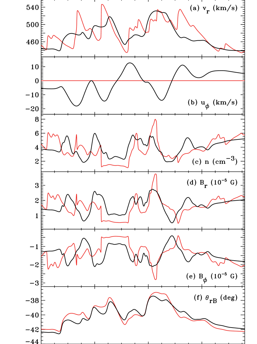
Figure 13.— Simulated time variability of the low-diffusion (red curves) and high-diffusion (black curves) models that would be seen by a spacecraft at 1 AU. Shown are: (a) radial wind speed $v_{r}$, (b) azimuthal speed in the inertial frame $u_{\phi}$, (c) proton number density $n$, (d) radial field strength $B_{r}$, (e) azimuthal field strength $B_{\phi}$, and (f) Parker spiral angle $\theta_{rB}$.

Figure 13 shows a summary of other plasma parameters at 1 AU, here plotted as a function of time as would be measured by a stationary spacecraft. We used Equation (3) to translate longitude into time, and for simplicity we normalized $t$ to zero at the left edge of the plot. Table 1 gives the mean values of several relevant parameters at 1 AU for the two models. One can see more clearly that the low-diffusion model contains sharper features, often with larger variability, that tend to be more smeared out in the high-diffusion model. The tight correlation between $B_{r}$ and $B_{\phi}$ is a preliminary indication that the dominant type of magnetic variability is in the magnitude of the field and not in its direction. Also, the modeled fluctuations in gas pressure and magnetic pressure are largely in phase with one another, and are not 180° out of phase like one would expect in pressure-balance structures (Burlaga et al., 1990; Tu & Marsch, 1994; Vasquez & Hollweg, 1999). These correlations are discussed further in Section 6. The Parker spiral angle is defined as $\theta_{rB}=\tan^{-1}(B_{\phi}/B_{r})$. Figure 13(f) shows that the pattern of longitudinal variability seen for $\theta_{rB}$ does not depend much on whether departures from strict corotation are included in $v_{\phi}$ (as in the high diffusion model) or not (as in the low diffusion model).

Table 1Modeled MHD Parameters at 1 AU

Parameter	High-diffusion Model	Low-diffusion Model
Mean $v_{r}$ (km s-1)	474.3	481.2
Mean $v_{\phi}$ (km s-1)	–400.2	–399.0
Mean $n$ (cm-3)	3.854	3.656
Mean $|{\bf B}|$ (nT)	2.169	2.072
Mean $\beta$ ($P_{\rm gas}/P_{\rm mag}$)	7.383	8.223
$E_{{\rm K},r}/E_{n}$	1.402	1.612
$E_{{\rm K},\phi}/E_{n}$	0.1407	0
$E_{{\rm B},r}/E_{n}$	0.06527	0.09566
$E_{{\rm B},\phi}/E_{n}$	0.04293	0.06724
$E_{\rm th}/E_{n}$	0.5919	1.131
Total $E/E_{n}$	2.243	2.906

We found it instructive to simulate global time-distance images from the MHD models and compare them to similar images constructed from observations of white-light heliospheric imagers. For example, the Sun Earth Connection Coronal and Heliospheric Investigation (SECCHI) on STEREO contains imagers that probe electron density fluctuations at distances of order 15–300 $R_{\odot}$ (Eyles et al., 2009). By stacking up radially oriented image slices taken over a range of times, one can visualize the mutual interactions of fast and slow streams, coronal mass ejections (CMEs), and shocks in a clear way (see, e.g., Davies et al., 2009; Rouillard et al., 2010; Howard & DeForest, 2012). Figure 14 shows the result, using the same time coordinate as in Figure 13 and using the mass density $\rho$ as the plotted grayscale quantity. At each height, the white and black limits of the grayscale map were redefined based on the local minimum and maximum density in $\phi$. Both the modeled and observed images show that fine-scale flux tube variations in the innermost heliosphere become smeared out by CIR-like stream interactions at larger distances.

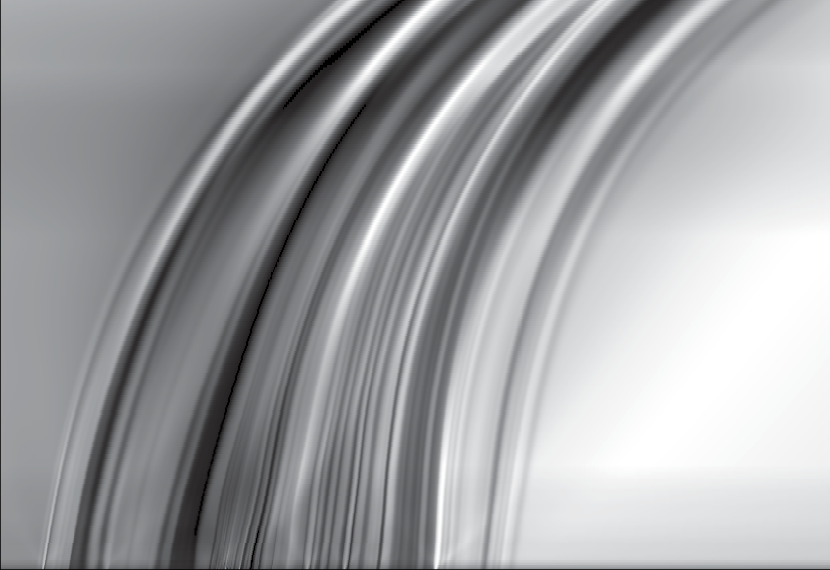
Figure 14.— Simulated time-distance variations of density fluctuations from the high-diffusion MHD model. The normalization of the horizontal time axis is the same as that used in Figure 13. Grayscale levels are defined independently at each radial distance to be proportional to relative electron density variations.

Many of the results discussed above are independent of the adopted value of the inner boundary distance. As discussed above, we chose 20 $R_{\odot}$ as a standard baseline. We wanted a value low enough that substantial stream interactions would not have already occurred, but high enough that most of the solar wind’s acceleration as modeled by ZEPHYR would be included. We also wanted to avoid the sub-Alfvénic region in which $u_{\phi}$ is undergoing a transition from rigid rotation to angular momentum conservation (Weber & Davis, 1967). In order to explore the sensitivity of the parameters at 1 AU to the boundary distance, we ran two other low-diffusion models with inner radii of 15 $R_{\odot}$ and 30 $R_{\odot}$. Because we did not fine-tune the polytropic $\gamma$ to reproduce the ZEPHYR code’s wind acceleration profile at large distances, we found that the mean wind speed $v_{r}$ at 1 AU does depend on the choice of inner radius. However, in all three models, the mean mass flux $\rho v_{r}$ and the mean radial field strength $B_{r}$ at 1 AU were nearly invariant (i.e., they differed by less than 1% from one another). Also, the relative fluctuations at 1 AU, measured by the ratios of standard deviations to mean values (for both $\rho$ and $v_{r}$) were nearly invariant across the three models.

6. Statistics of Modeled MHD Fluctuations

Because the two-dimensional models described above do not include any explicit time variability, the resulting “fluctuations” (as seen in, e.g., Figure 13) should not be expected to resemble propagating MHD waves or turbulent eddies. Nonetheless, it is useful to first examine them in the context of linear MHD wave theory. We determined the mean energy density components of the fluctuations at 1 AU,

$$E_{{\rm K},i}=\frac{\rho_{0}\langle v_{i}^{2}\rangle}{2}\,\,,\,\,\,\,E_{{\rm B},i}=\frac{\langle B_{i}^{2}\rangle}{8\pi}\,\,,\,\,\,\,E_{\rm th}=\frac{a_{0}^{2}\langle\rho^{2}\rangle}{2\rho_{0}}\,\,,$$ (14)

where quantities with subscript 0 refer to mean values taken over the 80° of fully resolved longitudes, quantities given as $\langle f^{2}\rangle$ refer to the variance of $f$ over the same range of longitudes, and the subscript $i$ refers to either the $r$ or $\phi$ vector components. The three terms above refer to kinetic, magnetic, and thermal fluctuations, respectively. Alfvénic fluctuations would be characterized by equipartition between the kinetic and magnetic components perpendicular to the background field. Magnetosonic waves tend to have half of their fluctuation energy in kinetic form and the other half divided between the magnetic and thermal terms (see Figure 2 of Cranmer & van Ballegooijen, 2012). Pressure-balance structures (PBSs) are largely static features that advect with the solar wind and carry along variations in gas pressure and magnetic pressure that are in rough equipartition between the $E_{\rm B}$ and $E_{\rm th}$ terms given above.

Table 1 gives the values of the fluctuation energy density components for the two models discussed in Section 5. Each energy density has been normalized by dividing by a representative 1 AU background magnetic energy density $E_{n}=B_{n}^{2}/8\pi$, where $B_{n}=2\times 10^{-5}$ G $=$ 2 nT. This value of $B_{n}$ was chosen to be of the same order of magnitude as the mean magnetic field strength at 1 AU in the models. Table 1 shows that both models had significantly more than half of their total energy in the form of kinetic fluctuations, which is inconsistent with both linear MHD waves and PBSs. Still, the models had an approximately magnetosonic balance between the relative rms variations in magnetic field amplitude ($\langle B^{2}\rangle^{1/2}/B_{0}$) and density ($\langle\rho^{2}\rangle^{1/2}/\rho_{0}$), with both ratios being roughly equal to 0.30 for the high-diffusion model and to 0.39 for the low-diffusion model. This may be a natural consequence of the frozen-in MHD assumption, since the spacing of field lines undergoes similar compressions and rarefactions as the gas.

The total modeled energy density in fluctuations was between 2 and 3 times the background value $E_{n}$. This can be compared with measured plasma fluctuations at 1 AU. The total energy density of reported MHD turbulence is roughly about 3–5 $E_{n}$ (e.g., Tu & Marsch, 1995; Goldstein et al., 1995; Bruno & Carbone, 2005), depending on the type of solar wind stream. This is in approximate agreement with the models, but we will see below that there are key differences between the detailed power spectra of the models and the observations. We also found that larger-scale fluctuations in the ecliptic plane contribute to a much higher energy density than do just the small-scale turbulent motions. For example, over the 16 days of OMNI data collected for Figure 12(d), the total energy density computed from all components of Equation (14) was found to be 42.4 $E_{n}$. Much of this (28.3 $E_{n}$) was in the kinetic energy variance due to alternating fast and slow streams. It is clear that the large-scale models presented here do not come close to reproducing the full range of MHD variability in the solar wind.

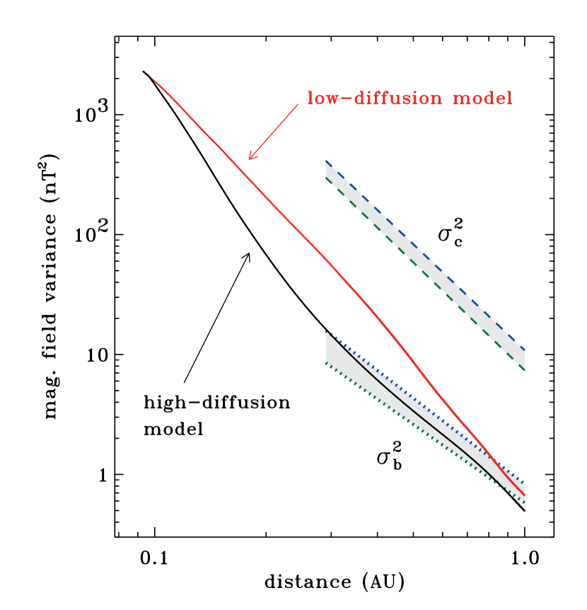
Figure 15.— Radial dependence of magnetic field variance in the inner heliosphere. For the low-diffusion model (red solid curve) and the high-diffusion model (black solid curve), plotted values of the component variance $\sigma_{c}^{2}$ are nearly identical to the magnitude variance $\sigma_{b}^{2}$ (not shown). These are compared with Helios measurements of $\sigma_{c}^{2}$ (dashed curves) and $\sigma_{b}^{2}$ (dotted curves) for data averaged over 12 hour bins (blue upper curves) and 3 hour bins (green lower curves).

We can learn more about how the models may reproduce some aspects of the actual solar wind by examining the radial evolution of the magnetic field fluctuations. Figure 15 shows the radial dependence of the “component variance” $\sigma_{c}^{2}$, which is the sum of the variances of the individual vector components of ${\bf B}$. For both the low-diffusion and high-diffusion models, this quantity is nearly identical to (i.e., within 5% of) the magnitude variance $\sigma_{b}^{2}$, which is the variance of the scalar field strength $|{\bf B}|$. We do not plot $\sigma_{b}^{2}$ for the models since the curves would be indistinguishable from the $\sigma_{c}^{2}$ curves.

Figure 15 also compares the model results with measurements made by Helios in the slow wind ($v\leq 500$ km s^-1). We show measured ranges for $\sigma_{c}^{2}$ and $\sigma_{b}^{2}$ given by Mariani et al. (1978) for two different methods of binning the data. In the real solar wind, $\sigma_{c}^{2}/\sigma_{b}^{2}\approx 10$, which indicates that the directional variations in the vector magnetic field greatly exceed the magnitude variations. Although our model does not contain the small-scale MHD waves that contribute to the observed $\sigma_{c}^{2}$, it does seem to reproduce the large-scale magnitude variations that contribute to $\sigma_{b}^{2}$. Thus, we make the conjecture that the low-frequency variability of magnetic field magnitude in the solar wind may be caused by the longitudinal interaction and evolution of coronal flux tubes.

Additional information about the nature of the modeled fluctuations can be extracted from their power spectra. Converting the longitudinal coordinate $\phi$ into time using Equation (3), we took fast Fourier transforms (FFTs) of various MHD quantities over the 80° of fully resolved longitude and plotted the power as a function of spacecraft-frame frequency. For example, Figure 16 shows power spectra of the fluctuations of radial velocity $v_{r}$ at both the inner boundary radius of 20 $R_{\odot}$ and at 1 AU. The curve at 20 $R_{\odot}$ is the same for the low-diffusion and high-diffusion models because the same ZEPHYR boundary condition was used for both. Despite the high resolution of the models, the numerically determined power spectra were extremely noisy. Thus, for clarity we plot 9-point boxcar-smoothed curves for all modeled spectra, and we show the full, unsmoothed spectrum for only one case: the inner boundary spectrum at 20 $R_{\odot}$. The smoothing does not alter the overall shape or magnitude of the spectrum.

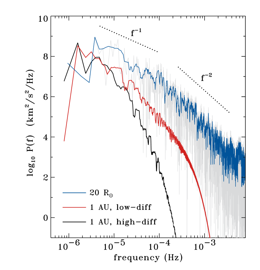
Figure 16.— Fourier power spectra of $v_{r}$ fluctuations in the time-steady MHD models. The raw FFT result for the inner boundary condition at 20 $R_{\odot}$ is shown (light gray curve) along with its 9-point boxcar smoothing average (blue curve). Corresponding smoothed spectra at 1 AU are shown for the low-diffusion model (red curve) and high-diffusion model (black curve).

The velocity power spectrum at 20 $R_{\odot}$ is roughly proportional to $f^{-1}$ for frequencies between about $5\times 10^{-6}$ and $10^{-4}$ Hz. This is reminiscent of—but probably not causally related to—the $f^{-1}$ spectrum seen for some quantities at frequencies below $10^{-4}$ Hz in the solar wind at 1 AU (Bavassano et al., 1982; Matthaeus & Goldstein, 1986; Nicol et al., 2009). The modeled spectrum steepens to roughly $f^{-2}$ at higher frequencies, and the steepening continues as the spectrum evolves outward in heliocentric distance. The high-diffusion model steepens more than the low-diffusion model. This is expected since the former model undergoes more longitudinal smearing of structure at small spatial scales (i.e., at high spacecraft-frame frequencies). The power at the very lowest frequencies ($f\lesssim 3\times 10^{-6}$ Hz, i.e., timescales greater than a few days) appears to grow with increasing heliocentric distance. Although there is no formal “inverse cascade” in this model, the transfer of energy from small to large scales can be the result of CIR-like stream collisions that eventually produce merged interaction regions (MIRs; e.g., Burlaga et al., 2003).

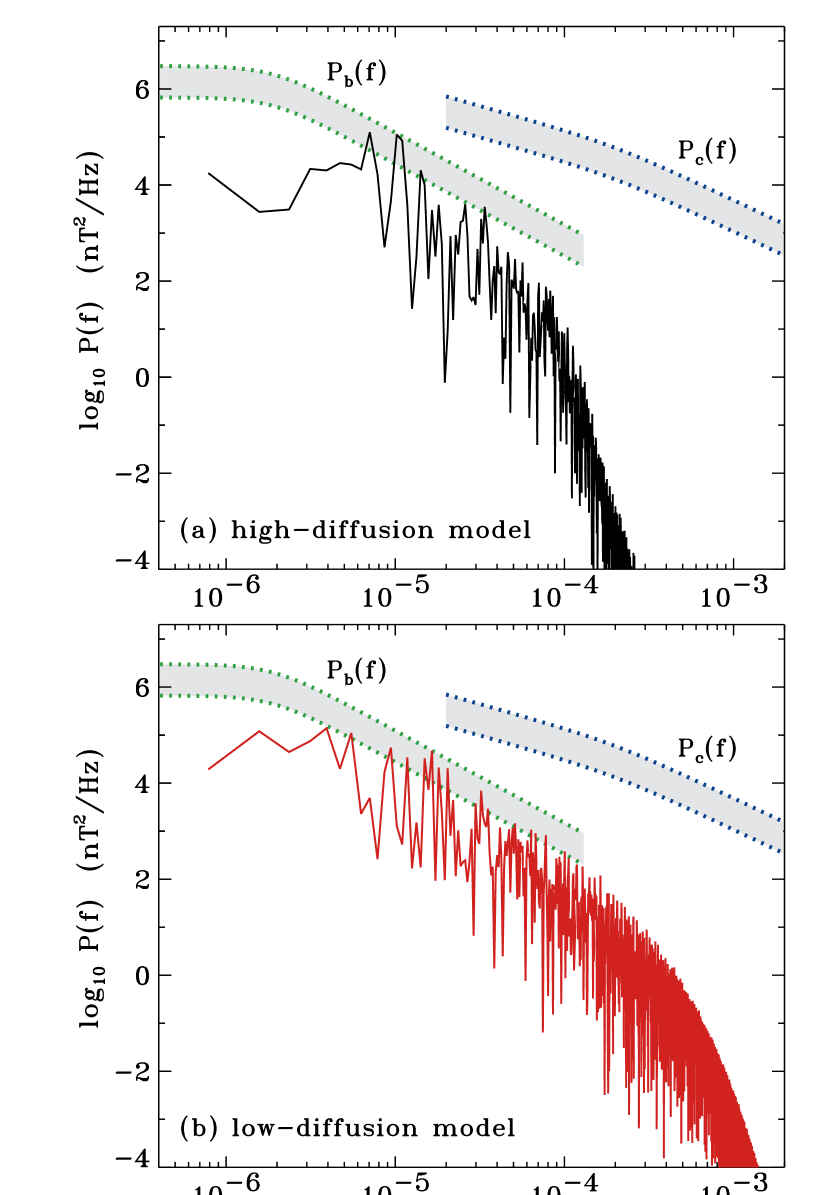
Figure 17.— Fourier power spectra of magnetic field fluctuations in the high-diffusion (a) and low-diffusion (b) models at 1 AU. Simulated power spectra (solid curves) are compared with measured ranges of vector component fluctuations (blue dotted curves) and scalar magnitude fluctuations (green dotted curves).

Figure 17 shows the modeled magnetic fluctuation power spectra at 1 AU without any boxcar smoothing. For clarity, the results of the low-diffusion and high-diffusion models are shown in separate panels. The gray regions give the ranges of measured magnetic power spectra for the slow solar wind in the ecliptic plane. The spectrum labeled $P_{c}(f)$ gives the “full” MHD turbulence spectrum that is analogous to the component variance $\sigma_{c}^{2}$ discussed above (see, e.g., Tu & Marsch, 1995; Matsui et al., 2002; Bruno & Carbone, 2005; Vasquez et al., 2007). The spectrum labeled $P_{b}(f)$ is the spectrum of fluctuations in the scalar field strength (Burlaga et al., 1989), and it is analogous to the magnitude variance $\sigma_{b}^{2}$. The agreement between the low-diffusion model spectrum and the measured range of $P_{b}(f)$ is quite good. This appears to reinforce our earlier suggestion that the proposed model of longitudinally evolving coronal flux tubes can explain the measured low-frequency fluctuations of magnetic field magnitude in the solar wind.

It is also evident from Figure 17 that the low-frequency $f^{-1}$ part of the measured fluctuation spectrum $P_{c}(f)$ contains significantly more power than is found in the modeled spectra at 1 AU. The $f^{-1}$ fluctuations are often claimed to be fossil remnants of coronal variations (e.g., Roberts, 2010). However, we can tentatively conclude from these simulations that if this is true, it is more likely for them to represent propagating waves and not just the “passive” survival of coronal flux tubes.

7. Discussion and Conclusions

The aim of this paper was to begin exploring how MHD fluctuations in interplanetary space are related to the well-known filamentary flux-tube structure of the solar corona. Starting with a time-steady potential-field model of the QS corona allowed us to model the properties of a “bundle” of open field lines with footpoint separations that extend down to scales smaller than those of both granules and intergranular lanes. This let us study magnetic field variations on spatial scales that are still unresolvable with state-of-the-art MHD simulations of the global corona and heliosphere. After adjusting the field strengths found from the PFSS approximation, we produced one-dimensional models of the coronal heating and solar wind acceleration along these field lines. These models assumed that the energization of the corona comes from the dissipation of MHD turbulence, but in principle any model of plasma heating could be applied. We also used the one-dimensional results as lower boundary conditions to a model of radial and longitudinal heliospheric evolution, and we predicted the time-steady formation of CIR structure from the coronal flux tubes. The resulting fluctuations in magnetic field magnitude greatly resemble corresponding fluctuations that have been measured in the low-latitude slow solar wind.

One original goal of this paper was to study the origin of low-frequency MHD fluctuations in the solar wind. Power spectra obeying a relatively flat $f^{-1}$ frequency dependence are often suggested to be the turbulent “energy containing range” and of direct solar origin, but their cause is still being debated (Matthaeus & Goldstein, 1986; Velli et al., 1989; Matthaeus et al., 2007; Dmitruk & Matthaeus, 2007; Dmitruk et al., 2011; Verdini et al., 2012b). There is also still disagreement over whether the statistical properties of MHD discontinuities are due to flux tubes of solar origin (Borovsky, 2010) or are the by-product of an ongoing turbulent cascade (Greco et al., 2008). Our ecliptic-plane models were not set up to reproduce inherently time-variable fluctuations, but they do help put limits on the ability of small-scale coronal variations to survive the effects of stream-stream CIR-type interactions. They also act as a basal level of expected background fluctuations to which must be added any propagating waves or turbulent motions. Interactions between waves and static structures have been invoked as possible means of mode conversion and coronal heating (e.g., Gogoberidze et al., 2007; Evans et al., 2012), so knowing more about the background variations is important to help constrain those theories.

As emphasized in Section 2, our time-steady description of the coronal magnetic field was meant only to be a snapshot that is representative of the high-resolution topology that exists at any one time (see also Jendersie & Peter, 2006). The validity of this kind of model depends crucially on the scales being resolved. Because the smallest structures will have the shortest lifetimes, it becomes increasingly necessary, when going to smaller scales, to take into account the evolving nature of the magnetic carpet. Cranmer & van Ballegooijen (2010), Meyer et al. (2012), and others presented Monte Carlo simulations that may be useful to “connect” to the solar wind acceleration models of this paper. At the very least, such simulations can be used to provide insight about how rapidly the field geometry evolves as a function of height. Of course, fully time-dependent and multidimensional techniques will be needed to describe the self-consistent interactions between flux tubes, waves, turbulent fluctuations, and fast/slow streams in the heliosphere.

We also note that our assumption of a potential field for extrapolating the measured photospheric magnetogram data into the corona is likely to be inaccurate in many key ways. Using an improved MHD treatment could naturally incorporate many of the non-potential effects that we attempted to account for in our $B_{2}$ enhancement term. In addition, the PFSS technique is known to eliminate nearly all of the smallest-scale longitudinal flux-tube structure in the field at and above the source surface. In our case, this resulted in an inability to test the alternate flux-tube expansion formalism of Fujiki et al. (2005) and Suzuki (2006), who suggested that $B_{\rm ss}\propto B_{\rm base}/f_{\rm ss}$ may be a better quantity to correlate with the wind speed than $f_{\rm ss}$ itself.

Despite the above warnings, we believe the high-resolution magnetic field models constructed for this paper can be useful tools for studying the statistical properties of spatial plasma fluctuations that exist sufficiently near the Sun that other effects (e.g., stream interactions or turbulence) do not smear them out. These variations can be compared straightforwardly to existing remote-sensing observations. For example, we would like to know if these inter-flux-tube variations contribute to the measured nonthermal widths of coronal emission lines (e.g., Gupta, 2010) or to the large velocity variances obtained from radio scintillation data (Harmon & Coles, 2005). Both of these are commonly interpreted as being caused by the line-of-sight integration through a corona filled by Alfvén waves, but the effects of “static” flux tubes remain to be disentangled. We would also like to simulate the MHD fluctuations at the intermediate distances to be probed by Solar Probe Plus ($r\gtrsim 0.05\,\mbox{AU}$) and Solar Orbiter ($r\gtrsim 0.28\,\mbox{AU}$). This requires a more self-consistent calculation of $u_{\phi}$ to model the turnover from rigid corotation to angular momentum conservation (e.g., Weber & Davis, 1967; Priest & Pneuman, 1974), and it may also require including “true” heating and acceleration source terms into the two-dimensional code described in Section 5.

Appendix A Potential Field Source Surface Model

In this paper we compute the magnetic field assuming the corona is current-free (i.e., a potential field). We use a spherical domain extending from the solar surface up to a radial distance $R_{\rm ss}$, where the field is assumed to be radial. Low resolution versions of such potential field source surface (PFSS) models have been used extensively in the past (e.g., Schatten et al., 1969; Altschuler & Newkirk, 1969; Wang & Sheeley, 1990; Arge & Pizzo, 2000; Luhmann et al., 2002; Wang & Sheeley, 2006). In the present work we need high spatial resolution in the low corona to accurately trace the roots of the open field lines on scales below $\sim$1 Mm in the photosphere. Using the standard method, which is based on spherical harmonic expansion, very large grids covering the entire Sun would be required. However, high resolution is needed only in a limited region on the solar surface. Therefore, we use a different computational method in which the high resolution grid extends only over some limited area. The basic methodology is described in Appendix B of van Ballegooijen et al. (2000), and can be summarized as follows. The magnetic field ${\bf B}({\bf r})$ is written in terms of a vector potential ${\bf A}({\bf r})$, which is given by

$$A_{r}\,=\,0\,,\,\,\,\,\,\,\,A_{\theta}\,=\,-\frac{1}{r\sin\theta}\frac{\partial\Psi}{\partial\phi}\,,$$ (A1)

$$A_{\phi}\,=\,\frac{1}{r}\left[\frac{\partial\Psi}{\partial\theta}+B_{0}\tan(\theta/2)\right]\,,$$ (A2)

where $(r,\theta,\phi)$ are spherical coordinates, $B_{0}$ is the monopole component of the imposed radial field, and $\Psi(r,\theta,\phi)$ is a scalar function that must satisfy the following partial differential equation:

$$\frac{\partial^{2}\Psi}{\partial r^{2}}+\nabla_{\perp}^{2}\Psi\,=\,0\,\,.$$ (A3)

The gradient operator $\nabla_{\perp}$ operates only on the coordinates perpendicular to the radial direction. Thus, the potential field is given by

$${\bf B}({\bf r})\,=\,B_{0}\left(\frac{R_{\sun}}{r}\right)^{2}\hat{\bf r}-\nabla\left(\frac{\partial\Psi}{\partial r}\right)\,\,.$$ (A4)

At the longitudinal boundaries of the high-resolution domain, $B_{\phi}$ either vanishes or is periodic in longitude; at the latitudinal boundaries we require $B_{\theta}=0$. Due to these boundary conditions, the solution of Equation (A3) can be written as a superposition of discrete eigenmodes, but the eigenmodes are not spherical harmonics and must be computed numerically. The mode amplitudes are chosen such that ${\bf B}({\bf r})$ matches the imposed radial magnetic field at the solar surface ($r=R_{\sun}$) and satisfies $\partial\Psi/\partial r=0$ at the source surface ($r=R_{\rm ss}$).

Two important improvements have been made to the basic method. First, we use a variable grid. At certain heights in the corona the grid spacing is doubled in all three directions, allowing us to cover the full height range of the model with a relatively small number of grid points (for details see Appendix A of Bobra et al., 2008). Second, a description of the global corona has been added to improve the side boundary conditions on the high-resolution domain (see Section 4.1 of Su et al., 2011). The high-resolution and global models are computed in such a way that the magnetic field is continuous across the side boundaries of the high-resolution domain. Hence, field lines can be traced through the side boundaries without any unphysical kinks in the field lines.

As described above, we used a SOLIS line-of-sight (LOS) photospheric magnetogram taken on 2003 September 4 at 16:30 UT, as well as the SOLIS synoptic map for the relevant Carrington Rotation (CR 2007). The LOS magnetogram was converted into a longitude-latitude map of the radial field $B_{r}(R_{\sun},\theta,\phi)$ in the high resolution part of the grid. This conversion assumes that the magnetic field on the Sun is nearly radial, which is a good approximation for the Quiet Sun. The high resolution grid has $1024\times 512$ cells on the photosphere, and the grid spacing is $0.0018\cos\lambda\,R_{\sun}$, where $\lambda$ is the latitude. The source surface is located at $R_{\rm ss}=2.46\,R_{\sun}$. The synoptic map from CR 2007 was used for constructing the global part of the PFSS model.

References

- Abbett (2007) Abbett, W. P. 2007, ApJ, 665, 1469
- Aiouaz & Rast (2006) Aiouaz, T., & Rast, M. P. 2006, ApJ, 647, L183
- Altschuler & Newkirk (1969) Altschuler, M. D., & Newkirk, G. 1969, Sol. Phys., 9, 131
- Antiochos et al. (2007) Antiochos, S. K., DeVore, C. R., Karpen, J. T., & Mikić, Z. 2007, ApJ, 671, 936
- Antiochos et al. (2011) Antiochos, S. K., Mikić, Z., Titov, V., Lionello, R., & Linker, J. 2011, ApJ, 731, 112
- Arge & Pizzo (2000) Arge, C. N., & Pizzo, V. J. 2000, J. Geophys. Res., 105, 10465
- Banaszkiewicz et al. (1998) Banaszkiewicz, M., Axford, W. I., & McKenzie, J. F. 1998, A&A, 337, 940
- Bastian et al. (1998) Bastian, T. S., Benz, A. O., & Gary, D. E. 1998, ARA&A, 36, 131
- Bavassano et al. (1982) Bavassano, B., Dobrowolny, M., Mariani, F., & Ness, N. F. 1982, J. Geophys. Res., 87, 3617
- Berger et al. (1995) Berger, T. E., Schrijver, C. J., Shine, R. A., et al. 1995, ApJ, 454, 531
- Bobra et al. (2008) Bobra, M. G., van Ballegooijen, A. A., & DeLuca, E. E.. 2008, ApJ, 672, 1209
- Borovsky (2008) Borovsky, J. E. 2008, J. Geophys. Res., 113, A08110
- Borovsky (2010) Borovsky, J. E. 2010, Phys. Rev. Lett., 105, 111102
- Bruno & Carbone (2005) Bruno, R., & Carbone, V. 2005, Living Rev. Solar Phys., 2, 4
- Burlaga et al. (2003) Burlaga, L. F., Berdichevsky, D., Gopalswamy, N., Lepping, R., & Zurbuchen, T. 2003, J. Geophys. Res., 108, 1425
- Burlaga et al. (1989) Burlaga, L. F., Mish, W. H., & Roberts, D. A. 1989, J. Geophys. Res., 94, 177
- Burlaga et al. (1990) Burlaga, L. F., Scudder, J. D., Klein, L. W., & Isenberg, P. A. 1990, J. Geophys. Res., 95, 2229
- Canfield et al. (1999) Canfield, R. C., Hudson, H. S., & McKenzie, D. E. 1999, Geophys. Res. Lett., 26, 627
- Chandran et al. (2011) Chandran, B. D. G., Dennis, T. J., Quataert, E., & Bale, S. D. 2011, ApJ, 743, 197
- Chitta et al. (2012) Chitta, L. P., van Ballegooijen, A. A., Rouppe van der Voort, L., DeLuca, E. E., & Kariyappa, R. 2012, ApJ, 752, 48
- Close et al. (2005a) Close, R. M., Parnell, C. E., Longcope, D. W., & Priest, E. R. 2005a, Sol. Phys., 231, 45
- Close et al. (2005b) Close, R. M., Parnell, C. E., & Priest, E. R. 2005b, Geophys. Astrophys. Fluid Dyn., 99, 513
- Cranmer (2008) Cranmer, S. R. 2008, ApJ, 689, 316
- Cranmer (2009) Cranmer, S. R. 2009, Living Rev. Solar Phys., 6, 3
- Cranmer (2010) Cranmer, S. R. 2010, ApJ, 710, 676
- Cranmer et al. (2009) Cranmer, S. R., Matthaeus, W. H., Breech, B. A., & Kasper, J. C. 2009, ApJ, 702, 1604
- Cranmer & Saar (2011) Cranmer, S. R., & Saar, S. H. 2011, ApJ, 741, 54
- Cranmer & van Ballegooijen (2005) Cranmer, S. R., & van Ballegooijen, A. A. 2005, ApJS, 156, 265
- Cranmer & van Ballegooijen (2010) Cranmer, S. R., & van Ballegooijen, A. A. 2010, ApJ, 720, 824
- Cranmer & van Ballegooijen (2012) Cranmer, S. R., & van Ballegooijen, A. A. 2012, ApJ, 754, 92
- Cranmer et al. (2007) Cranmer, S. R., van Ballegooijen, A. A., & Edgar, R. J. 2007, ApJS, 171, 520
- Davies et al. (2009) Davies, J. A., Harrison, R. A., Rouillard, A. P., et al. 2009, Geophys. Res. Lett., 36, L02102
- DeForest et al. (2005) DeForest, C. E., Hassler, D. M., & Schwadron, N. A. 2005, Sol. Phys., 229, 161
- Dmitruk & Matthaeus (2007) Dmitruk, P., & Matthaeus, W. H. 2007, Phys. Rev. E, 76, 036305
- Dmitruk et al. (2011) Dmitruk, P., Mininni, P. D., Pouquet, A., Servidio, S., & Matthaeus, W. H. 2011, Phys. Rev. E, 83, 066318
- Einaudi et al. (1999) Einaudi, G., Boncinelli, P., Dahlburg, R. B., & Karpen, J. T. 1999, J. Geophys. Res., 104, 521
- Evans et al. (2012) Evans, R. M., Opher, M., Oran, R., van der Holst, B., Sokolov, I. V., Frazin, R., Gombosi, T. I., & Vásquez, A. 2012, ApJ, 756, 155
- Eyles et al. (2009) Eyles, C. J., Harrison, R. A., Davis, C. J., et al. 2009, Sol. Phys., 254, 387
- Fisk et al. (1999) Fisk, L. A., Schwadron, N. A., & Zurbuchen, T. H. 1999, J. Geophys. Res., 104, 19765
- Fujiki et al. (2005) Fujiki, K., Hirano, M., Kojima, M., et al. 2005, Adv. Sp. Res., 35, 2185
- Gabriel (1976) Gabriel, A. H. 1976, Phil. Trans. Roy. Soc., A281, 339
- Garraffo et al. (2012) Garraffo, C., Cohen, O., Drake, J. J., & Downs, C. 2012, ApJ, in press, arXiv:1212.2226
- Gary et al. (1987) Gary, G. A., Moore, R. L., Hagyard, M. J., & Haisch, B. M. 1987, ApJ, 314, 782
- Ghosh al. (2009) Ghosh, S., Thomson, D. J., Matthaeus, W. H., & Lanzerotti, L. J. 2009, J. Geophys. Res., 114, A08106
- Giacalone et al. (2006) Giacalone, J., Jokipii, J. R., & Matthaeus, W. H. 2006, ApJ, 641, L61
- Giovanelli (1980) Giovanelli, R. G. 1980, Sol. Phys., 68, 49
- Gogoberidze et al. (2007) Gogoberidze, G., Rogava, A., & Poedts, S. 2007, ApJ, 664, 549
- Goldstein et al. (1995) Goldstein, M. L., Roberts, D. A., & Matthaeus, W. H. 1995, ARA&A, 33, 283
- Gosling (1996) Gosling, J. T. 1996, ARA&A, 34, 35
- Greco et al. (2008) Greco, A., Chuychai, P., Matthaeus, W. H., Servidio, S., & Dmitruk, P. 2008, Geophys. Res. Lett., 35, L19111
- Güdel (2007) Güdel, M. 2007, Living Rev. Solar Phys., 4, 3
- Gupta (2010) Gupta, G. R., Banerjee, D., Teriaca, L., Imada, S., & Solanki, S. 2010, ApJ, 718, 11
- Hackenberg et al. (2000) Hackenberg, P., Marsch, E., & Mann, G. 2000, A&A, 360, 1139
- Hagenaar et al. (2008) Hagenaar, H. J., De Rosa, M. L., & Schrijver, C. J. 2008, ApJ, 678, 541
- Hammer (1982) Hammer, R. 1982, ApJ, 259, 767
- Harmon & Coles (2005) Harmon, J. K., & Coles, W. A. 2005, J. Geophys. Res., 110, A03101
- He et al. (2007) He, J.-S., Tu, C.-Y., & Marsch, E. 2007, A&A, 468, 307
- Henney et al. (2009) Henney, C. J., Keller, C. U., Harvey, J. W., et al. 2009, in ASP Conf. Proc. 405, Solar Polarization 5, ed. S. V. Berdyugina, K. N. Nagendra, R. Ramelli (San Francisco: ASP), 47
- Hoeksema & Scherrer (1986) Hoeksema, J. T., & Scherrer, P. H. 1986, Sol. Phys., 105, 205
- Hollweg (1974) Hollweg, J. V. 1974, J. Geophys. Res., 79, 3845
- Hollweg (1976) Hollweg, J. V. 1976, J. Geophys. Res., 81, 1649
- Holzer et al. (1983) Holzer, T. E., Flå, T., & Leer, E. 1983, ApJ, 275, 808
- Howard & DeForest (2012) Howard, T. A., & DeForest, C. E. 2012, ApJ, 746, 64
- Hu (1993) Hu, Y. Q. 1993, J. Geophys. Res., 98, 13201
- Jacques (1977) Jacques, S. A. 1977, ApJ, 215, 942
- Jendersie & Peter (2006) Jendersie, S., & Peter, H. 2006, A&A, 460, 901
- Jian et al. (2011) Jian, L. K., Russell, C. T., Luhmann, J. G., et al. 2011, Sol. Phys., 273, 179
- Keller et al. (2003) Keller, C. U., Harvey, J. W., & the SOLIS Team 2003, in ASP Conf. Proc. 307, Solar Polarization, ed. J. Trujillo-Bueno & J. Sanchez Almeida (San Francisco: ASP), 13
- Kovalenko (1981) Kovalenko, V. A. 1981, Sol. Phys., 73, 383
- Lee et al. (2009) Lee, C. O., Luhmann, J. G., Odstrcil, D., et al. 2009, Sol. Phys., 254, 155
- Leer & Holzer (1980) Leer, E., & Holzer, T. E. 1980, J. Geophys. Res., 85, 4631
- Leer et al. (1982) Leer, E., Holzer, T. E., & Flå, T. 1982, Space Sci. Rev., 33, 161
- Luhmann et al. (2002) Luhmann, J. G., Li, Y., Arge, C. N., Gazis, P. R., & Ulrich, R. 2002, J. Geophys. Res., 107, 1154
- Mariani et al. (1978) Mariani, F., Ness, N. F., Burlaga, L. F., Bavassano, B., & Villante, U. 1978, J. Geophys. Res., 83, 5161
- Mariani & Neubauer (1990) Mariani, F., & Neubauer, F. M. 1990, in Physics of the Inner Heliosphere, ed. R. Schwenn & E. Marsch (Berlin: Springer), 183
- Matsui et al. (2002) Matsui, H., Farrugia, C. J., & Torbert, R. B. 2002, J. Geophys. Res., 107, 1355
- Matthaeus et al. (2007) Matthaeus, W. H., Breech, B., Dmitruk, P., Bemporad, A., Poletto, G., Velli, M., & Romoli, M. 2007, ApJ, 657, L121
- Matthaeus et al. (1995) Matthaeus, W. H., Gray, P. C., Pontius, D. H., Jr., & Bieber, J. W. 1995, Phys. Rev. Lett., 75, 2136
- Matthaeus & Goldstein (1986) Matthaeus, W. H., & Goldstein, M. L. 1986, Phys. Rev. Lett., 57, 495
- Matthaeus et al. (1999) Matthaeus, W. H., Zank, G. P., Oughton, S., Mullan, D. J., & Dmitruk, P. 1999, ApJ, 523, L93
- McCracken & Ness (1966) McCracken, K. G., & Ness, N. F. 1966, J. Geophys. Res., 71, 3315
- McComas et al. (1998) McComas, D. J., Bame, S. J., Barker, P., et al. 1998, Space Sci. Rev., 86, 563
- McGregor et al. (2011) McGregor, S. L., Hughes, W. J., Arge, C. N., Owens, M. J., & Odstrcil, D. 2011, J. Geophys. Res., 116, A03101
- McIntosh & De Pontieu (2009) McIntosh, S. W., & De Pontieu, B. 2009, ApJ, 707, 524
- Meyer et al. (2012) Meyer, K. A., Mackay, D. H., & van Ballegooijen, A. A. 2012, Sol. Phys., 278, 149
- Moore et al. (2011) Moore, R. L., Sterling, A. C., Cirtain, J. W., & Falconer, D. A. 2011, ApJ, 731, L18
- Mullan (1991) Mullan, D. J. 1991, A&A, 248, 256
- Neugebauer et al. (1995) Neugebauer, M., Goldstein, B. E., McComas, D. J., Suess, S. T., & Balogh, A. 1995, J. Geophys. Res., 100, 23389
- Nicol et al. (2009) Nicol, R. M., Chapman, S. C., & Dendy, R. O. 2009, ApJ, 703, 2138
- Nisenson et al. (2003) Nisenson, P., van Ballegooijen, A. A., de Wijn, A. G., & Sütterlin, P. 2003, ApJ, 587, 458
- Owens et al. (2005) Owens, M. J., Arge, C. N., Spence, H. E., & Pembroke, A. 2005, J. Geophys. Res., 110, A12105
- Parhi et al. (1999) Parhi, S., Suess, S. T., & Sulkanen, M. 1999, J. Geophys. Res., 104, 14781
- Petrosyan et al. (2010) Petrosyan, A., Balogh, A., Goldstein, M. L., Léorat, J., Marsch, E., Petrovay, K., Roberts, B., von Steiger, R., & Vial, J. C. 2010, Space Sci. Rev., 156, 135
- Pneuman (1980) Pneuman, G. W. 1980, A&A, 81, 161
- Press et al. (1992) Press, W. H., Teukolsky, S. A., Vetterling, W. T., & Flannery, B. P. 1992, Numerical Recipes in Fortran: The Art of Scientific Computing (Cambridge: Cambridge Univ. Press)
- Priest & Pneuman (1974) Priest, E. R., & Pneuman, G. W. 1974, Sol. Phys., 34, 231
- Reardon et al. (2011) Reardon, K. P., Wang, Y.-M., Muglach, K., & Warren, H. P. 2011, ApJ, 742, 119
- Reisenfeld et al. (1999) Reisenfeld, D. B., McComas, D. J., & Steinberg, J. T. 1999, Geophys. Res. Lett., 26, 1805
- Riley (2007) Riley, P. 2007, J. Atmos. Sol. Terr. Phys., 69, 32
- Riley & Lionello (2011) Riley, P., & Lionello, R. 2011, Sol. Phys., 270, 575
- Riley & Luhmann (2012) Riley, P., & Luhmann, J. G. 2012, Sol. Phys., 277, 355
- Roberts (2010) Roberts, D. A. 2010, ApJ, 711, 1044
- Rouillard et al. (2010) Rouillard, A. P., Davies, J. A., Lavraud, B., et al. 2010, J. Geophys. Res., 115, A04103
- Schatten et al. (1969) Schatten, K. H., Wilcox, J. M., & Ness, N. F. 1969, Sol. Phys., 6, 442
- Schrijver et al. (2005) Schrijver, C. J., De Rosa, M. L., Title, A. M., & Metcalf, T. R. 2005, ApJ, 628, 501
- Schrijver & van Ballegooijen (2005) Schrijver, C. J., & van Ballegooijen, A. A. 2005, ApJ, 630, 552
- Smith & Wolfe (1976) Smith, E. J., & Wolfe, J. H. 1976, Geophys. Res. Lett., 3, 137
- Steiner et al. (2001) Steiner, O., Hauschildt, P. H., & Bruls, J. 2001, A&A, 372, L13
- Su et al. (2011) Su, Y., Surges, V., van Ballegooijen, A., DeLuca, E., & Golub, L. 2011, ApJ, 734, 53
- Suzuki (2006) Suzuki, T. K. 2006, ApJ, 640, L75
- Thieme et al. (1990) Thieme, K. M., Marsch, E., & Schwenn, R. 1990, Ann. Geophys., 8, 713
- Tian et al. (2011) Tian, H., McIntosh, S. W., Habbal, S. R., & He, J. 2011, ApJ, 736, 130
- Title and Schrijver (1998) Title, A. M., & Schrijver, C. J. 1998, in ASP Conf. Proc. 154, 10th Cambridge Workshop on Cool Stars, Stellar Systems and the Sun, ed. R. Donahue & J. Bookbinder (San Francisco: ASP), 345
- Tu & Marsch (1994) Tu, C.-Y., & Marsch, E. 1994, J. Geophys. Res., 99, 21481
- Tu & Marsch (1995) Tu, C.-Y., & Marsch, E. 1995, Space Sci. Rev., 73, 1
- van Ballegooijen et al. (2000) van Ballegooijen, A. A., Priest, E. R., & Mackay, D. H. 2000, ApJ, 539, 983
- Vasquez & Hollweg (1999) Vasquez, B. J., & Hollweg, J. V. 1999, J. Geophys. Res., 104, 4681
- Vasquez et al. (2007) Vasquez, B. J., Smith, C. W., Hamilton, K., MacBride, B. T., & Leamon, R. J. 2007, J. Geophys. Res., 112, A07101
- Velli et al. (1989) Velli, M., Grappin, R., & Mangeney, A. 1989, Phys. Rev. Lett., 63, 1807
- Velli et al. (2011) Velli, M., Lionello, R., Linker, J. A., & Mikić, Z. 2011, ApJ, 736, 32
- Verdini et al. (2012a) Verdini, A., Grappin, R., & Velli, M. 2012a, A&A, 538, A70
- Verdini et al. (2012b) Verdini, A., Grappin, R., Pinto, R., & Velli, M. 2012b, ApJ, 750, L33
- Wang & Sheeley (1990) Wang, Y.-M., & Sheeley, N. R., Jr. 1990, ApJ, 355, 726
- Wang & Sheeley (1991) Wang, Y.-M., & Sheeley, N. R., Jr. 1991, ApJ, 372, L45
- Wang & Sheeley (2003) Wang, Y.-M., & Sheeley, N. R., Jr. 2003, ApJ, 587, 818
- Wang & Sheeley (2006) Wang, Y.-M., & Sheeley, N. R., Jr. 2006, ApJ, 653, 708
- Wang et al. (1997) Wang, Y.-M., Sheeley, N. R., Jr., Phillips, J. L., & Goldstein, B. E. 1997, ApJ, 488, L51
- Weber & Davis (1967) Weber, E. J., & Davis, L., Jr. 1967, ApJ, 148, 217
- Whang (1980) Whang, Y. C. 1980, J. Geophys. Res., 85, 2285
- Wiegelmann & Solanki (2004) Wiegelmann, T., & Solanki, S. K. 2004, Sol. Phys., 225, 227
- Wiegelmann et al. (2010) Wiegelmann, T., Solanki, S. K., Borrero, J. M., et al. 2010, ApJ, 723, L185
- Withbroe (1988) Withbroe, G. L. 1988, ApJ, 325, 442
- Woolsey & Cranmer (2012) Woolsey, L. N., & Cranmer, S. R. 2012, Eos Trans. AGU, Fall Meet. Suppl., abstract SH33D-2252
- Yamauchi et al. (2002) Yamauchi, Y., Suess, S. T., & Sakurai, T. 2002, Geophys. Res. Lett., 29, 1383
- Yeates et al. (2010) Yeates, A. R., Mackay, D. H., van Ballegooijen, A. A., & Constable, J. A. 2010, J. Geophys. Res., 115, A09112
- Zank et al. (1996) Zank, G. P., Matthaeus, W. H., & Smith, C. W. 1996, J. Geophys. Res., 101, 17093
- Zhang & Liu (2011) Zhang, J., & Liu, Y. 2011, ApJ, 741, L7
- Zhao et al. (2009) Zhao, M., Wang, J.-X., Jin, C.-L., & Zhou, G.-P. 2009, Research Astron. Astrophys., 9, 933