Transport Properties for Triangular Barriers
in Graphene Nanoribbon

Abderrahim El Mouhafid^a and Ahmed Jellal^a,b,c

^aTheoretical Physics Group, Faculty of Sciences, Chouaïb Doukkali University,

24000 El Jadida, Morocco

^bSaudi Center for Theoretical Physics, Dhahran, Saudi Arabia

^cPhysics Department, College of Sciences, King Faisal University,
Alahssa 31982, Saudi Arabia

We theoretically study the electronic transport properties of Dirac fermions through one and double triangular barriers in graphene nanoribbon. Using the transfer matrix method, we determine the transmission, conductance and Fano factor. They are obtained to be various parameters dependent such as well width, barrier height and barrier width. Therefore, different discussions are given and comparison with the previous significant works is done. In particular, it is shown that at Dirac point the Dirac fermions always own a minimum conductance associated with a maximum Fano factor and change their behaviors in an oscillatory way (irregularly periodical tunneling peaks) when the potential of applied voltage is increased.

PACS numbers: 72.80.Vp, 73.21.-b, 71.10.Pm, 03.65.Pm

Keywords: graphene, scattering, triangular potential, transmission.

1 Introduction

Graphene is a single two-dimensional array of carbon atoms with a honeycomb lattice, which was discovered in 2004 [1]. This finding has been attracted an intensive attention from both experimental and theoretical aspects. In particular, the tunneling of Dirac fermions in graphene has already been verified experimentally [2], which in turn has spurred an extraordinary amount of interest in the investigation of the electronic transport properties in graphene based quantum wells, barriers, p n junctions, transistors, quantum dots, superlattices, etc. The electrostatic barriers in graphene can be generated in various ways [3, 4]. For example, it can be done by applying a gate voltage, cutting it into finite width nanoribbons and using doping or otherwise. Whereas magnetic barrier can, in principle, can be realized by using magnetic strips or using superconductors [5]. As far graphene, results of the transmission coefficient and the tunneling conductance were already reported for the electrostatic barriers[4, 9, 6, 10, 7, 8] and magnetic barriers [11, 12, 13].

The electronic band structure (energy dispersion relation) of graphene consists of two inequivalent pairs of cones with apices located at Brillouin-zone corners. The dispersion relation $E=\pm\hbar v_{F}|\vec{k}|$ is linear around the Dirac point ($K$, $K^{\prime}$) where $v_{F}\simeq 10^{6}$m/s is Fermi velocity [14]. The presence of such Dirac-like quasiparticles is expected to induce some unusual electronic properties, which make difference with respect to two-dimensional electronic gas, such as the so-called Klein paradox [15], anomalous integer quantum Hall effect [16, 17, 18] and observation of minimum conductivity [17]. The fact that in an ideal graphene sheet the carriers are massless, gives rise to Klein paradox, which allows particles to tunnel through any electrostatic potential barriers, that is the wavefunction has an oscillatory tail outside the electrostatic barrier region. Hence this property excludes the possibility to confine electrons using electrostatic gates, as in usual semiconductors. Thus to enable the fabrication of confined structures, such as quantum dots, we need to use another type of barrier such as the infinite mass barrier [19].

Theoretical investigations have been widely performed to clarify the resonant-tunneling features using mostly barriers of the rectangular forms. The reasons because the corresponding models are so simple to have an advantage for numerical calculations. However few works studied tunneling effect with barriers of the potential slopes as a result of externally applied field [20, 21, 22, 23]. One of them is the trapezoidal double barrier structure, which was investigated to study the effect of the potential disturbance at the interfaces of the graphene cheet [24]. In the same spirit, we consider another problem based on single and double triangular barrier structures. Our model is possibly applied to the resonant tunneling diodes of which the barriers are formed by delta doping in the future and is also a step outward from a rectangular form from the other point of view. We ensure the confinement of Dirac fermions in the $y$-direction by using infinite mass confinement, which requires infinite mass at the boundary of the $y$-strip and results in a specific quantization of the $y$-component of the momentum [19]. The effects of the well width, barrier height and barrier width on the transport properties are systematically studied through numerical calculations. As long as the applied potential is increased, the number of the minimum conductance associated with maximum Fano factor increases as well. This result makes difference with respect to that of rectangular barrier where there is only one minimum and one maximum [10]. We conclude that it is relatively more easily for Dirac fermions to tunnel through a triangular barrier in a graphene sheet rather than rectangular one.

The outline of the paper is the following. In section 2, we set our theoretical model by giving the appropriate equation describing Dirac fermions in graphene and choosing the convenient configuration for the triangle double barrier structures as depicted in Figure 1. In section 3, we expose the exact analytical solution to solve the Dirac equation in each regions of the structures, which resulted in giving the corresponding eigenvalues and eigenspinors. Tunneling probabilities are calculated in section 4 as a functions of different parameters such as the fermion energy, static electric field and incident angle. These are done by matching spinors in different interfaces and using the transfer matrix techniques. In section 5, we discuss the transport results corresponding to single and double barriers separately. The obtained results show characteristic oscillations associated with tunneling resonances as a function of the fermion energy and the static electric field. We conclude our work in the final section.

2 Theoretical formulation

We consider a system of massless Dirac fermions through a strip of graphene characterized by the length $L_{B}$ and width $w$ in the presence of a double triangular barriers. In the systems made of graphene, the two Fermi points, each with a two-fold band degeneracy, can be described by a low-energy continuum approximation with a four-component envelope wavefunction whose components are labeled by a Fermi-point pseudospin $=\pm 1$ and a sublattice forming an honeycomb. Being a zero-gap semiconductor, the quasiparticle motion can be described by the massless Dirac like equation

$$[v_{F}\vec{\sigma}\cdot\vec{p}+V(x)]\psi(x,y)=\varepsilon\psi(x,y)$$ (1)

where $v_{F}\simeq 9.84\times 10^{6}m/s$ is the Fermi velocity, $\vec{p}=-i\hbar\overrightarrow{\nabla}$ is the momentum operator (hereafter $v_{F}=\hbar=1$), $\vec{\sigma}=(\sigma_{x},\sigma_{y})$ are the Pauli matrices, $\varepsilon=\hbar v_{F}|\vec{k}|$ being the energy of the incident particle. A triangular double barrier configuration is depicted in Figure 1 with all parameters, which requires two kinds of width: the right and left sides of the barrier. Therefore the dependence of the various parameters can be considered as shown in the potential $V(x)$ configuration

$$V(x)=\left\{\begin{array}[]{ll}(x-a)F_{1},&\qquad x\in[a,b]\\ (x-c)F_{2},&\qquad x\in[b,c]\\ (x-d)F_{3},&\qquad x\in[d,e]\\ (x-f)F_{4},&\qquad x\in[e,f]\\ 0,&\qquad{\mbox{otherwise}}\end{array}\right.$$ (7)

where we have set $F_{1}=\frac{V_{1}}{b-a}$, $F_{2}=\frac{V_{1}}{b-c}$, $F_{3}=\frac{V_{2}}{e-d}$ and $F_{4}=\frac{V_{2}}{e-f}$ are the strength of the static electric field in each regions.

Our system is supposed to have finite width $w$ with infinite mass boundary conditions on the wavefunction at the boundaries $y=0$ and $y=w$ along the $y$-direction [7, 8, 11, 12, 13, 19]. This boundary conditions result in a quantization of the transverse momentum along the $y$-direction, which is

$$k_{y}=k_{n}=\frac{\pi}{w}\left(n+\frac{1}{2}\right),\qquad n=0,1,2\cdots.$$ (8)

Figure 1: The parameters of a triangle double barrier structure.

One can therefore assume a spinor solution of the following form $\psi_{j}(x,y)=(\phi_{j_{+}}(x),\phi_{j_{-}}(x))^{t}e^{ik_{y}y}$ where $j=1$ for $x<a$, $2$ for $x\in[a,b]$, $3$ for $x\in[b,c]$, $4$ for $x\in[c,d]$, $5$ for $x\in[d,e]$, $6$ for $x\in[e,f]$ and $7$ for $x>f$ denotes the different space regions. Thus our problem reduces to an effective $1D$ problem whose Dirac equation can be written as

$$\left(\begin{array}[]{cc}{V(x)-\varepsilon}&{\frac{d}{dx}+k_{y}}\\ {-\frac{d}{dx}+k_{y}}&{V(x)-\varepsilon}\end{array}\right)\left(\begin{array}[]{c}{\phi_{j_{+}}(x)}\\ {-i\phi_{j_{-}}(x)}\end{array}\right)=0.$$ (13)

An electron which impinges from $x=-\infty$ on the quantum barrier is partially reflected, partially transmitted at the interface $x=a$. Inside the barrier regions $[a,c]$ and $[d,f]$, the eigenstates is a combination of the parabolic cylinder functions waves. For $x>f$, the carrier is also partly transmitted and escapes towards $x=\infty$ with a wavevector $+k_{x}$. The electric potentials $F_{1}$, $F_{2}$, $F_{3}$ and $F_{4}$, being uniform along the $y$-direction, the $y$-component of momentum is conserved throughout the regions. Due to the space dependence of the potential $V(x)$ we make the following transformation on our spinor components to enable us to obtain Schrodinger like equations for each component, $\chi_{j_{+}}=\frac{1}{2}\left(\phi_{j_{+}}+\phi_{j_{-}}\right)$ and $\chi_{j_{-}}=\frac{1}{2i}\left(\phi_{j_{+}}-\phi_{j_{-}}\right)$, which obey the coupled stationary equations. These are

$$\frac{d}{dx}\chi_{j_{\pm}}(x)\pm i\left(V(x)-\epsilon\right)\chi_{j_{\pm}}(x)\mp ik_{{y}}\chi_{{j_{\mp}}}(x)=0.$$ (14)

Each spinor component $\chi_{j_{\pm}}$ can be shown to satisfy the following uncoupled second order differential equation

$$\frac{d^{2}}{d{x}^{2}}\chi_{{j_{\pm}}}(x)+\left(\pm i{\frac{d}{dx}}V(x)+\left[V(x)-\varepsilon\right]^{2}-{k_{y}}^{2}\right)\chi_{{j_{\pm}}}(x)=0.$$ (15)

At this stage, we point out that our effective $2D$ massless Dirac equation (13) is equivalent to a massive one with an effective mass $m$ equal to the transverse quantized wave vector $k_{y}$, i.e. $m=k_{y}=k_{n}$. For this purpose, we consider a unitary transformation, which enable us to map the effective $2D$ massless equation into a $1D$ massive Dirac equation. Such a unitary transformation does not affect the energy spectrum or the physics of the problem. We choose a rotation by $\pi/4$ about the $y$-axis, $U=e^{i\frac{\pi}{4}\sigma_{y}}$ and thus the transformed Hamiltonian and wavefunction read

$$\left(\begin{array}[]{cc}{V(x)-\varepsilon+k_{y}}&{\frac{d}{dx}}\\ {-\frac{d}{dx}}&{V(x)-\varepsilon-k_{y}}\end{array}\right)\left(\begin{array}[]{c}{\tilde{\psi}^{j}_{+}(x)}\\ {}\hfil\\ {\tilde{\psi}^{j}_{-}(x)}\end{array}\right)=0, \qquad\tilde{\psi}_{j_{+,-}}(x)=U\psi_{j_{+,-}}(x).$$ (21)

which is identical to a $1D$ massive Dirac equation with an effective mass $m^{\ast}=k_{y}$. This shows clearly how to derive the dynamical mass generation via space compactification [23] from our model

3 Exact solution

After solving the differential equation (15), It turns out its solution in regions $x<a$, $[c,d]$ and $x>f$ are given by

$$\phi_{1}(x) = \left(\begin{array}[]{c}1\\ z_{n,k_{x}}\\ \end{array}\right)e^{ik_{x}x}+r_{n}\left(\begin{array}[]{c}1\\ -z^{\ast}_{n,k_{x}}\\ \end{array}\right)e^{-ik_{x}x}$$ (26)

$$\phi_{4}(x) = \alpha_{n4}\left(\begin{array}[]{c}u^{+}_{4}(x)\\ u^{-}_{4}(x)\\ \end{array}\right)+\beta_{n4}\left(\begin{array}[]{c}v^{+}_{4}(x\\ v^{-}_{4}(x\\ \end{array}\right),$$ (31)

$$\phi_{7}(x) = t_{n}\left(\begin{array}[]{c}1\\ z_{n,k_{x}}\\ \end{array}\right)e^{ik_{x}x},$$ (34)

where $r_{n}$ and $t_{n}$ are the reflection and transmission amplitudes, respectively, ${n}$ is labeling the modes, the functions $u^{\pm}_{4}(x)$ and $v^{\pm}_{4}(x)$ are $u^{+}_{4}(x)=v^{+^{\ast}}_{4}(x)=u^{-}_{4}(x)/z=-v^{-^{\ast}}_{4}(x)=e^{ik_{x}x}$. The wavevector $k_{x}=\sqrt{\varepsilon^{2}-k_{y}^{2}}$ and the complex number $z_{n,k_{x}}$ is defined as

$$z_{n,k_{x}}=\mbox{sgn}(\varepsilon)\frac{k_{x}+ik_{n}}{\sqrt{k_{x}^{2}+k_{n}^{2}}}$$ (35)

where the transversal momenta is quantized as shown in (8). Note that this quantization is the result of the infinite mass boundary conditions mentioned previously on the wavefunction along the $y$-direction. In the case of $|k_{y}|>|\varepsilon|$, the waves are evanescent (bound states) outside and inside the quantum barrier and thus the imaginary wavevectors associated with the evanescent waves are given by $k_{x}=i\sqrt{k_{y}^{2}-\varepsilon^{2}}$. Since we are interested by the transmission of relativistic particles (continuum scattering states), thus we disregard the bound states which correspond to imaginary $k_{x}$.

The solution of (15) in the quantum barrier (region $[a,b]$) can be expressed in terms of the parabolic cylinder function $D_{\nu}(x)$ as

$$\chi_{2_{+}}(x)=\alpha_{n2}D_{\nu_{n1}-1}\left(q_{1}\right)+\beta_{n2}D_{-\nu_{n1}}\left(-q_{1}^{\ast}\right)$$ (36)

where $\nu_{n1}=\frac{ik_{n}^{2}(a-b)}{2V_{1}}$, $q_{1}=\sqrt{\frac{2}{(a-b)V_{1}}}e^{i\pi/4}(V_{1}x+E_{1})$, $E_{1}=-aV_{1}+(a-b)\varepsilon$, the parameters $\alpha_{n2}$ and $\beta_{n2}$ are constants. Now substituting (36) into (14) to get the second component of $\chi_{2}(x)$

$$\chi_{2_{-}}(x) = \alpha_{n2}\frac{-1}{(a-b)k_{n}}\sqrt{2(a-b)V_{1}}e^{-i\pi/4}D_{\nu_{n1}}\left(q_{1}\right)$$

$$+ \beta_{n2}\frac{1}{(a-b)k_{n}}[-\sqrt{2(a-b)V_{1}}e^{i\pi/4}D_{1-\nu_{n1}}\left(-q_{1}^{\ast}\right)2(-V_{1}x-E_{1})D_{-\nu_{n1}}\left(-q_{1}^{\ast}\right)].$$

The components of the spinor solution of the Dirac equation (7) in the region $[a,b]$ can be obtained from (36) and (3) with $\phi_{2_{+}}(x)=\chi_{2_{+}}+i\chi_{2_{-}}$ and $\phi_{2_{-}}(x)=\chi_{2_{+}}-i\chi_{2_{-}}$. These give

$$\phi_{2}(x)=\alpha_{n2}\left(\begin{array}[]{c}u_{2}^{+}(x)\\ u_{2}^{-}(x)\\ \end{array}\right)+\beta_{n2}\left(\begin{array}[]{c}v_{2}^{+}(x)\\ v_{2}^{-}(x)\\ \end{array}\right)$$ (38)

where the functions $u_{2}^{\pm}(x)$ and $v_{2}^{\pm}(x)$ read as

$$u_{2}^{\pm}(x) = \mp\sqrt{\frac{2V_{1}}{a-b}}\frac{1}{k_{n}}e^{i\pi/4}D_{\nu_{n1}}\left(q_{1}\right)+D_{\nu_{n1}-1}\left(q_{1}\right)$$

$$v_{2}^{\pm}(x) = \frac{1}{(a-b)^{3/2}k_{n}}[\pm\sqrt{2V_{1}}(a-b)e^{-i\pi/4}D_{-\nu_{n1}+1}\left(-q_{1}^{\ast}\right)$$

$$+ \sqrt{a-b}\left(b(\pm 2i\varepsilon-k_{n})-a(\pm k_{n}+2i(V_{1}-\varepsilon))\mp 2iV_{1}x\right)D_{-\nu_{n1}}\left(-q_{1}^{\ast}\right)]$$

Similarly, the solution of (15) in the region $[b,c]$ takes the form

$$\chi_{3_{+}}(x)=\alpha_{n3}D_{\nu_{n2}}\left(q_{2}\right)+\beta_{n3}D_{-\nu_{n2}-1}\left(-q_{2}^{\ast}\right)$$ (40)

where $\nu_{n2}=\frac{ik_{n}^{2}(b-c)}{2V_{1}}$, $q_{2}=\sqrt{\frac{2}{(b-c)V_{1}}}e^{i\pi/4}(V_{1}x+E_{2})$, $E_{2}=-cV_{1}+(c-b)\varepsilon$. The other component of $\chi_{3}(x)$ is given by

$$\chi_{3_{-}}(x) = \alpha_{n2}\frac{1}{(b-c)k_{n}}[-\sqrt{2(b-c)V_{1}}e^{-i\pi/4}D_{\nu_{2}+1}\left(q_{2}\right)+2(V_{1}x+E_{2})D_{\nu_{n2}}\left(q_{2}\right)]$$ (41)

$$+ \beta_{n2}\frac{-1}{(b-c)k_{n}}\sqrt{2(b-c)V_{1}}e^{i\pi/4}D_{-\nu_{n2}}\left(-q_{2}^{\ast}\right).$$

Combining (40) and (41) in similar way to ${\phi_{2}(x)}$, we obtain the eigenspinor solution of the Dirac equation (7) in the region $[b,c]$

$$\phi_{3}(x)=\alpha_{n3}\left(\begin{array}[]{c}u_{3}^{+}(x)\\ u_{3}^{-}(x)\\ \end{array}\right)+\beta_{n3}\left(\begin{array}[]{c}v_{3}^{+}(x)\\ v_{3}^{-}(x)\\ \end{array}\right)$$ (42)

where we have set

$$u_{3}^{\pm}(x) = \frac{1}{(b-c)^{3/2}k_{n}}[\mp\sqrt{2V_{1}}(b-c)e^{i\pi/4}D_{\nu_{n2}+1}\left(q_{2}\right)$$ (43)

$$+ \sqrt{b-c}\left(b(\mp 2i\varepsilon+k_{n})-c(k_{n}+2i(\pm V_{1}\mp\varepsilon))\pm 2iV_{1}x\right)D_{\nu_{n2}}\left(q_{2}\right)]$$

$$v_{3}^{\pm}(x) = \pm\sqrt{\frac{2V_{1}}{b-c}}\frac{1}{k_{n}}e^{-i\pi/4}D_{-\nu_{n2}}\left(-q_{2}^{\ast}\right)+D_{-\nu_{n2}-1}\left(-q_{2}^{\ast}\right)$$

Finally, note that the general solution of equation (15) in regions $[d,e]$ and $[e,f]$ can be obtained by interchanging $a\rightarrow d$, $b\rightarrow e$, $c\rightarrow f$ and $V_{1}\rightarrow V_{2}$ in the equations (3) and (43). The coefficients $r_{n}$, $t_{n}$, $\alpha_{nj}$ and $\beta_{nj}$ ($j=2,3,5,6$) can be determined by matching wavefunction at different interfaces.

4 Transport properties

The transmission coefficient is determined by imposing the continuity of the wavefunction at the interfaces between regions. This procedure is most conveniently expressed in the transfer matrix formalism. Here we directly use this approach and refer the reader to references [25, 26] for a detailed discussion. The transfer matrix defined by

$$\hat{M}=\left(\begin{array}[]{cc}M_{11}&M_{12}\\ M_{21}&M_{21}\end{array}\right)$$ (46)

relates the wavefunction on the left side of the barrier structure $(\phi_{{x<a}})$ to that on the right side $(\phi_{{x>f}})$. We can then construct $2\times 2$ matrices in each region, whose columns are given by the spinor solutions, such as for regions (1,4,7)

$$w_{1}(x)=w_{4}(x)=w_{7}(x)=\left(\begin{array}[]{cc}e^{ik_{x}x}&e^{-ik_{x}x}\\ z_{n,k_{x}}e^{ik_{x}x}&-z^{\ast}_{n,k_{x}}e^{-ik_{x}x}\end{array}\right)$$ (49)

and for $j={2},3,5,6$

$$w_{j}(x)=\left(\begin{array}[]{cc}u_{j}^{+}(x)&v_{j}^{+}(x)\\ u_{j}^{-}(x)&v_{j}^{-}(x)\end{array}\right)$$ (50)

These matrices play the role of partial transfer matrices and allow to express the continuity condition of the wavefunction at each interface. Note that the components of matrices $w_{5}(x)$ and $w_{6}(x)$ can be obtained by interchanging $a\rightarrow d$, $b\rightarrow e$ and $c\rightarrow f$ in matrices $w_{2}(x)$ and $w_{3}(x)$, respectively. After straightforward algebra, we get the transfer matrix as function of different boundaries

$$\hat{M}=w_{1}^{-1}(a)w_{2}(a)w_{2}^{-1}(b)w_{3}(b)w_{3}^{-1}(c)w_{1}(c)w_{1}^{-1}(d)w_{5}(d)w_{5}^{-1}(e)w_{6}(e)w_{6}^{-1}(f)w_{1}(f)$$ (51)

and the relation which expresses the continuity of the wavefunction is then given by

$$\left(\begin{array}[]{c}1\\ r_{n}\\ \end{array}\right)=\hat{M}\left(\begin{array}[]{c}t_{n}\\ 0\\ \end{array}\right).$$ (56)

Solving equation (56) for the transmission amplitude $t_{n}$ of the $n$th wave mode through the barrier, we get the transmission probability $T_{n}$ as

$$T_{n}=\left|t_{n}\right|^{2}=\frac{1}{\left|M_{11}\right|^{2}}.$$ (57)

Based on [27], we give a review about the shot noise. Indeed, the conductance of a single transmission channel can be written as

$$G=g\frac{e^{2}}{h}T$$ (58)

where $g$ is the degeneracy (spin and valley) of the system and $T$ the electron transmission probability. When the system is biased, shot noise appears due to discreteness of charge [28] and these current fluctuations for a single channel are given by

$$\langle(\delta I)^{2}\rangle=2e\langle I\rangle(1-T).$$ (59)

The total noise power spectrum for a multichannel conductor is then obtained by summing over all $N$ transmission eigenchannels:

$$S_{I}=\frac{2e^{3}|V|}{h}\sum^{N_{\sf{max}}-1}_{n=0}T_{n}(1-T_{n}).$$ (60)

In the limit of low transparency $T_{n}\ll 1$,

$$S_{I}\cong S_{\sf Poisson}=\frac{2e^{3}|V|}{h}\sum^{N-1}_{n=0}T_{n}=2e\langle I\rangle$$ (61)

defining a Poissonian noise induced by independent and random electrons like in tunnel junctions [28]. The regular way to quantify shot noise is to use the Fano factor $F$ which is the ratio between the measured shot noise and the Poissonian noise:

$$F=\frac{S_{I}}{S_{\sf Poisson}}=\frac{S_{I}}{2e\langle I\rangle}=\frac{\sum^{N-1}_{n=0}T_{n}(1-T_{n})}{\sum^{N-1}_{n=0}T_{n}}.$$ (62)

Then, for a Poissonian process $F=1$ at small transparency $(T_{n}\rightarrow 0)$, while $F=0$ in the ballistic regime (i.e. when $T_{n}\rightarrow 1$) and $F=1/3$ in the case of a diffusive system [10, 29, 30, 31].

In graphene, it has been theoretically concluded that transport at the Dirac point occurs via electronic evanescent waves [32, 10]. Tworzydlo et al. [10] used heavily-doped graphene leads and the wavefunction matching method to directly solve the Dirac equation in perfect graphene with length $L_{B}$ and width $w$. They found that for armchair edges, the quantization condition of the transverse wave vector is defined by

$$k_{y,n}=\frac{(n+\alpha)}{w}\pi$$ (63)

where $\alpha=0$ or $1/3$ for metallic and semiconducting armchair edges, respectively. At the Dirac point, the transmission coefficients are given by [10]

$$T_{n}=\frac{1}{\cosh\left(\pi\left(n+\alpha\right)\frac{L_{B}}{w}\right)}.$$ (64)

Consequently, graphene has a similar bimodal distribution of transmission eigenvalues at the Dirac point as there is in diffusive systems [33, 34]. In the limit of $w/L_{B}\rightarrow\infty$, the mode spacing becoming small and one can replace the sum over the channels by an integral over the transverse wave vector component $k_{y}$ to obtain the conductivity and the Fano factor for a sheet with metallic armchair edge [10]

$$\sigma_{\sf Dirac} = G\frac{L_{B}}{w}=\frac{4e^{2}}{h}\frac{L_{B}}{w}\int^{\infty}_{0}\frac{dk_{y}}{\cosh^{2}(k_{y}L_{B})}=\frac{4e^{2}}{\pi h}$$ (65)

$$F_{\sf Dirac} = \frac{\sum^{N-1}_{n=0}T_{n}(1-T_{n})}{\sum^{N-1}_{n=0}T_{n}}=\frac{1}{3}.$$ (66)

In summary, we will study the above quantities for the present system in terms of our findings and compare with already published works. In fact, the conductivity and the Fano factor of Dirac fermions through one and double triangular barriers in graphene will have a variate and different from with respect to the results presented in (65) and (66).

5 Results and discussions

For a better understanding of the obtained results so far, we numerically analysis different physical quantities in terms of the system parameters. To underline their behaviors, we trait single and double triangular barriers, separately.

5.1 Single barrier

We start our discussion by studying the transmission probability and shot noise for the Dirac fermions scattered by a single triangular barrier potential. We implement our previous analytical approaches to a graphene system subject to a single triangular barrier potential of strength $V_{1}$ and $V_{2}=0$. We will see that the transmission coefficient has a rich information about the electronic transport properties of the Dirac fermions through a triangular barrier structure.

The variations of the calculated transmission coefficient $T$ in terms of the incident electron energy $\varepsilon$ and applied voltage $V_{0}$ is displayed in Figure 2 for different values of the barrier widths $L_{B1}$, barrier widths right side $L_{1r}$, barrier heights $V_{0}$ and incident electron energy $\varepsilon$. From Figure 2, one can see that for certain values of $L_{B1}$ (Figure 2a), $V_{0}$ (Figure 2b) and $L_{1r}$ (Figure 2c), the transmission resonances appear in the triangular potential for $m^{\ast}<\varepsilon<V_{0}+2m^{\ast}$ and vanishes for both conditions ($\varepsilon>V_{0}$, $L_{1r}\neq L_{1l}$). We note that the intensity of resonances increase as long as $V_{0}$ and $L_{B1}$ increase, which allow for emergence of peaks in the $T$ shape. One can see that $T$ always starts from the energy corresponding to $k_{y}=m^{\ast}$, with $m^{\ast}$ is the effective mass of the $1D$ Dirac fermion. The zone when we have the energy such as $\varepsilon<m^{\ast}$ corresponds to the forbidden zone. It is important to note that the resonant energy depends strongly on the barrier height and width. For $L_{B1}=4$ we have the transmission resonances independtly of the value taken by the applied potentail $V_{0}$ as long as $V_{0}<\varepsilon$. While for $V_{0}>\varepsilon-2m^{\ast}$, the resonances decrease sharply until reach a relative minimum and then begin to increase in an oscillatory manner.

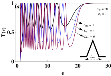
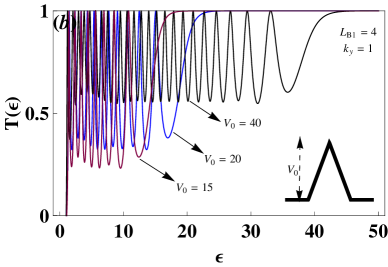
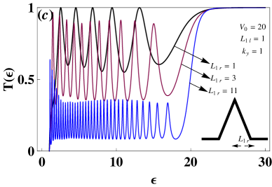
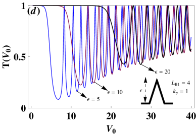
Figure 2: Transmission coefficient $T$ for the Dirac fermion scattered by a single triangular barrier potential with $V_{1}=V_{0}$ and $V_{2}=0$. (a), (b) and (c) as a function of incident electron energy, (d) as a function of applied voltage. ”Color figure online”

Figure 3 is showing the transmission coefficient $T$ as function of the electron incident angle $\phi$ for $\varepsilon=2$ and different values of ($V_{0}$, $L_{B1}$, $L_{1r}$). We see that the perfect transmission occurs at different angles and vice versa. It is observed that, the transmission is always total for a normal incidence angle. For $V_{0}=5$ one can observe that $T$ is not zero for some values of the barrier width. In particular it shows up two peaks at incident angles $\phi=\pm\frac{\pi}{3.6877}$ and $\phi=\pm\frac{\pi}{3.1469}$ for each value of the barrier widths $L_{B1}=10$ and $L_{B1}=4$, respectively. The transmission resonances always appear for the case of the barrier width only of the right side $L_{1r}$ is equal to the barrier width only of the left side $L_{1l}$, i.e. $L_{1r}=L_{1l}$, while disappear otherwise $(L_{1r}\neq L_{1l})$.

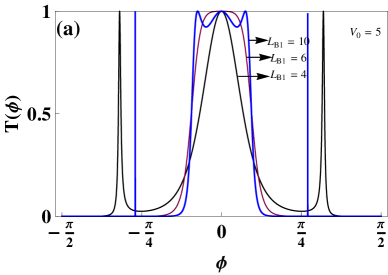
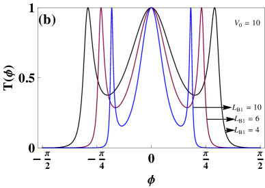
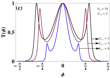
Figure 3: Transmission coefficient $T$ as a function of electron incident angle $\phi$ for the Dirac fermion scattered by a single triangular barrier potential with $V_{1}=V_{0}$, $V_{2}=0$ and $\varepsilon=2$. ”Color figure online”

In what follows we discuss the conductivity $\sigma$ and Fano factor $F$ behaviors to underline what makes difference with [17, 10, 35]. Indeed in Figure 4,

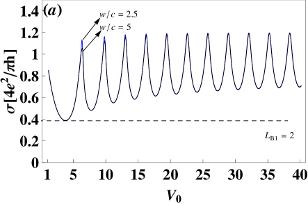
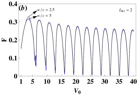
Figure 4: The electrostatic potential dependence of the Fano factor and the conductivity for the Dirac fermion scattered by a single triangular barrier potential with $V_{1}=V_{0}$, $V_{2}=0$, and $\varepsilon=2$. ”Color figure online”

we plot $\sigma$ (in units of $4e^{2}/\pi h$) and $F$ in terms of the electrostatic potential $V_{0}$ for $L_{B1}=2$ and $\varepsilon=2$. It is interesting to note that $\sigma$ corresponding to our system is showing some differences with respect to that for an ideal strip of graphene [10], which supports perfect transmission regardless of the barrier height (Klein tunneling [3]). It is obvious to observe that the conductivity and Fano factor change their behavior in an oscillatory way (irregularly periodical tunneling peaks) when we augment the potential of applied voltage. One can see that as long as $V_{0}$ increases, the number of minimum of $\sigma$ increases as well but the associated number of maximum of $F$ decreases. This effect is different from that obtained in [10] where there is only one minimum conductance $4e^{2}/(\pi h)$ at the Dirac point and for a geometric factor $w/L_{B}=5$, which corresponds to one maximum Fano factor $1/3$. In contrast, in our case for the same factor ($w/L_{B}=5$) the minimum conductivity 0.387 appears around $V_{0}=3.661$ where the associated maximum Fano factor is 0.315. More importantly, for two values of $V_{0}$ like $3.661$ and $7.616$ one can see that the minimum conductivity increases from 0.387 to 0.479. Consequently, both the potential barrier height and width for the particles emission can be reduced and then they can easily tunnel through the full barrier width, causing a larger field emission current. Therefore, we conclude that it is relatively more easily for the Dirac fermions to tunnel through a triangular barrier in a graphene sheet rather than rectangular one. It should be pointed out that the nonzero minimum conductance, as shown in Figure 4, may due to the conservation of pseudospin and the chiral nature of the relativistic particles in the graphene nanoribbon.

5.2 Double barriers

In this section we implement our previous analytical approach to a graphene system subject to a double triangular barrier potentials $V_{1}$ and $V_{2}$ so that the resulting static electric field strengths are

$$F_{1}=\frac{V_{1}}{l_{1l}},\qquad F_{2}=-\frac{V_{1}}{l_{1r}},\qquad F_{3}=\frac{V_{2}}{l_{2l}},\qquad F_{4}=-\frac{V_{2}}{l_{2r}}.$$ (67)

Note that there are various parameters involved such as well width, barrier height and barrier width, these will offer different discussions about transport properties in the present configuration of potential. In particular, Figures 5 and 6 show the transmission coefficient

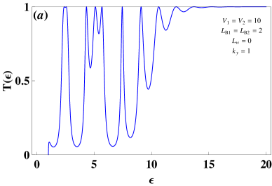
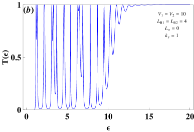
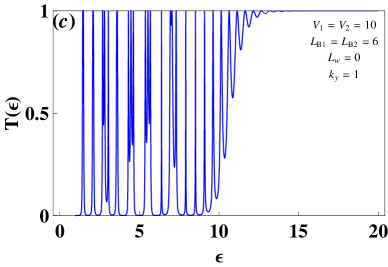
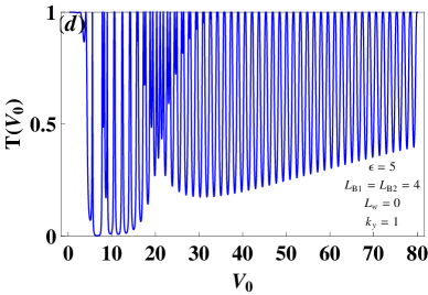
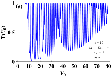
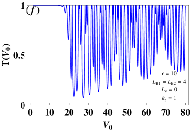
Figure 5: Transmission coefficient $T$ for the Dirac fermion scattered by a double triangular barriers potential with $V_{1}=V_{2}=V_{0}$, $L_{w}=0$ and $L_{B1}=L_{B2}$. (a), (b) and (c) as a function of incident electron energy, (d), (e) and (f) as a function of applied voltage. ”Color figure online”

in terms of the incident electron energy $\varepsilon$ and applied voltage $V_{1}=V_{2}=V_{0}$ for both cases $L_{w}=0$ and $L_{w}\neq 0$, with $L_{w}$ is the interbarrier separation (well width). In Figure 5, one can see that contrary to single barrier (e.g. Figure 2c) the transmission resonances always appear for double triangular barrier case. Clearly, the intensity and width of resonances as well as the condition for the existence of resonances depend on the static electric field strengths ($F_{1}$, $F_{2}$, $F_{3}$, $F_{4}$) and barrier widths ($L_{B1}$, $L_{B2}$). The intensity of resonances increases and decreases as long as the strengths ($\left|F_{1}\right|$, $\left|F_{2}\right|$, $\left|F_{3}\right|$, $\left|F_{4}\right|$) decrease and widths ($L_{B1}$, $L_{B2}$) increase, respectively.

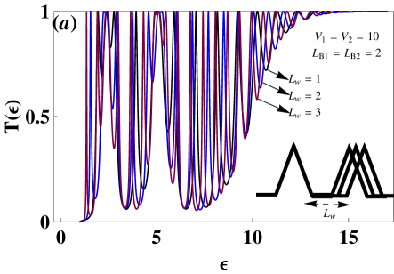
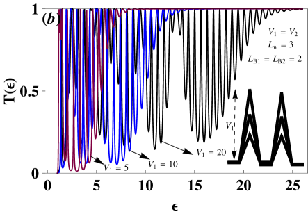
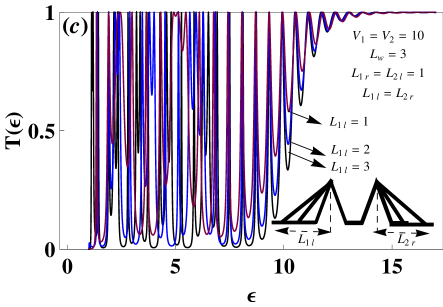
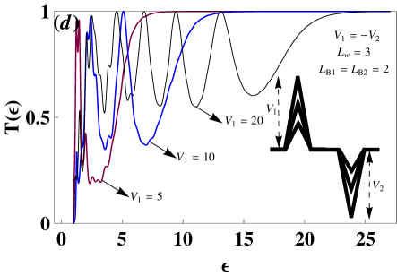
Figure 6: Transmission coefficient $T$ as a function of incident electron energy for the Dirac fermion scattered by a double triangular barriers potential with $V_{1}=|V_{2}|$ and $k_{y}=1$. (a) the width of the well was varied, (b) the barrier height is varied, (c) the barrier width only of the outer sides is varied, (d) the height of the barrier and the well is varied. ”Color figure online”

In Figure 6 we consider the same behavior of transmission as before but with $L_{w}\neq 0$. Compared to Figure 5 for $V_{1}=V_{2}=10$, one can conclude that the intensity of resonances depends strongly on $L_{w}$. In addition for $V_{1}=V_{2}$ there are several peaks showing transmission resonances those correspond to the bound states and no resonances exist for $V_{1}=-V_{2}$. Figure 6a presents three potential profiles and their transmission coefficients in terms of $\varepsilon$ for $L_{w}=1,2,3$, $L_{B1}=L_{B2}=2$ and $V_{1}=V_{2}=10$. The results show that as long as the well width $L_{w}$ increases the resonance peak structures become sharpened. We consider in Figure 6b the case of three values of barrier height ($V_{1}=V_{2}=5,10,20$) for $L_{B1}=L_{B2}=2$ and $L_{w}=3$. As the barrier height is enhanced, the transmission resonance shifts and the width of the resonances increases. The case of the double barriers is more important when the outer slopes of the barriers are varied with a fixed barrier height as shown in Figure 6c. We notice that the well region and the inner slope region are not changed when the parameters ($L_{1l}=L_{2r}$) vary. As long as the barrier becomes thick and high the resonance shifts toward the higher and the peak is more sharpened. Similarly to one triangular barrier, no resonance exists for the incident electron energy higher than $V_{1}+2m^{\ast}$ and the zone $\varepsilon<m^{\ast}$ is a forbidden zone. Except that when $V_{1}=-V_{2}$ no resonances exist for the following cases ($1<\varepsilon<9,V_{1}=-V_{2}=5$), ($1<\varepsilon<5,V_{1}=-V_{2}=10$) and ($1<\varepsilon<4.5,V_{1}=-V_{2}=20$), which are clearly shown in Figure 6d.

We represent in Figure 7 the transmission coefficient versus the incident angle with the same parameters as in Figure 3 for the Dirac fermion scattered by double triangular barriers potential with the interbarrier separation $L_{w}=0$. By contrast with the case for the Dirac fermion scattered by a single triangular barrier potential we conclude that the transmission resonances still always exist. The comparison between these two types of potential shows that for double barriers of strength $V_{1}=V_{2}=5$ we have three peaks with two peaks at incident angles

$$\phi=\pm\frac{\pi}{4.8021},\qquad\phi=\pm\frac{\pi}{3.6877}$$ (68)

and one peak at

$$\phi=\pm\pi$$ (69)

for each value of the barrier widths $L_{B1}=10$ and $L_{B1}=4$, respectively. Even though the barrier width only of the right side $L_{1r}$ is different to the barrier width only of the left side $L_{1l}$ for double barriers, the transmission resonances always appear contrary to the Dirac fermion scattered by a single barrier. We observe that decreasing the barrier width only of the right side the transmission coefficient takes relevant values for a wider set of incident angles.

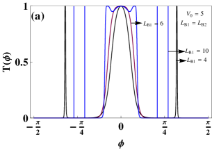
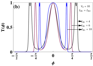
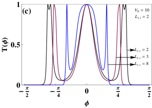
Figure 7: Transmission coefficient $T(\phi)$ for the Dirac fermion scattered by a double triangular barriers potential with $V_{1}=V_{2}=V_{0}$, $L_{w}=0$ and $\varepsilon=2$. ”Color figure online”

Finally, we close our discussion about transmission resonances by making comparison with the results reported for double barrier in graphene subjected to an external magnetic field in [36]. In fact, it was shown that increasing the magnetic field leads to a shift of transmission cone (a reduction of the number of resonances) and a shrinking of the perfect transmission region. However in our present study as we noticed before, the intensity of resonances increases and decreases as long as the static electric field strengths $(|F_{1}|,|F_{2}|,|F_{3}|,|F_{4}|)$ decrease and barrier widths $(L_{B_{1}},L_{B_{2}})$ increase, respectively.

As far as the conductivity and Fano factor behaviors for double barriers are concerned, we notice that the shot noise is characterized by the maximum of peaks at the minimums of conductivity and minimum of valleys at the maximums of conductivity. The role of the interbarrier separation $L_{w}$ resulted in increasing peaks of shot noise and lowering the current of valleys as shown in Figure 8. One can see that the value $F=1/3$ for the Dirac fermion scattered by double barriers is reproduced in the case where the barrier widths $L_{B1}=L_{B2}=2$, the interbarrier separation $L_{w}=0$ and the applied voltage $V_{0}$ near the $2\varepsilon$.

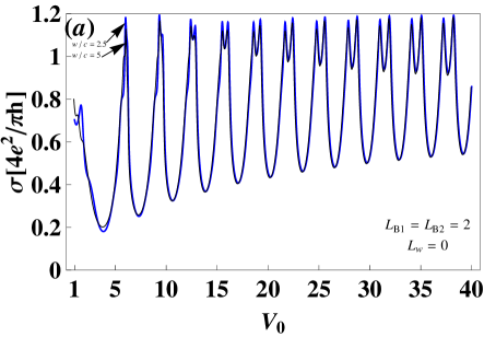
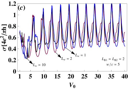
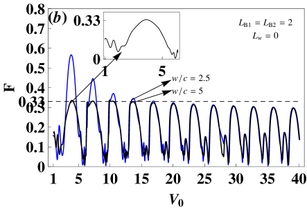
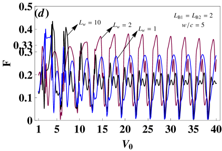
Figure 8: The electrostatic potential dependence of the Fano factor and the conductivity for the Dirac fermion scattered by a double triangular barriers potential with $V_{1}=V_{2}=V_{0}$, and $\varepsilon=2$. ”Color figure online”

6 Conclusion

We have analyzed the behavior of Dirac fermions in graphene submitted to electrostatic potential of triangular type. By solving the eigenvalue equation we have obtained the solutions of the energy spectrum in terms of different physical parameters involved in the Hamiltonian system. Using the continuity of the wavefunctions at the interfaces between regions inside and outside the barriers, we have studied the transport properties of the present system. More precisely, using the transfer matrix method, we have analyzed the corresponding transmission coefficient, conductivity and Fano factor for single and double triangular barriers.

It has been shown that the Dirac fermions scattered by single triangular and double triangular barriers own a minimum conductivity associated with a maximum Fano factor. We have noticed that the Dirac fermions can tunnel more easily through a barrier in the triangular forms rather than in the rectangular one. On the other hand, the behavior of the conductivity and the Fano factor in terms of the applied voltage showed irregular periodical oscillating for triangular potential.

We have noticed that the resonant energy is influenced by the barrier width. Indeed, when the barrier becomes thick and/or high, the resonant peak becomes sharpened and shifted to the higher energy. Even if the thickness and the height of the barriers are constant, the form of the triangular barrier affects the resonant energy. On the contrary, the triangular double barriers structures is less sensitive to the well width compared with a rectangular double barrier structure. Therefore, we have concluded that it is relatively more easily for the Dirac fermions to tunnel through a triangular barrier in a graphene sheet rather than rectangular one. These results may be helpful to deeply understand the transport in the nanoribbons and design the graphene-based nanodevices.

We close by mentioning that the obtained results can be extended to deal with other issues related to graphene systems. Indeed, one may think to study the transport properties of Dirac fermions scattered by periodical potentials and other types. Another interesting problem, what about a generalization of the obtained results to bilayer graphene and related matter.

References

- [1] K.S. Novoselov, A.K. Geim, S.V. Morozov, D. Jiang, Y. Zhang, S.V. Dubonos, I.V. Grigorieva and A.A. Firsov, Science 306 (2004) 666.
- [2] N. Stander, B. Huard and D. Goldhaber-Gordon, Phys. Rev. Lett. 102 (2009) 026807.
- [3] M.I. Katsnelson, K.S. Novoselov and A.K. Geim, Nature Phys. 2 (2006) 620.
- [4] H. Sevincli, M. Topsakal and S. Ciraci, Phys. Rev. B 78 (2008) 245402.
- [5] W. Van Roy, J. De Boeck and G. Borghs, Appl. Phys. Lett. 61 (1992) 3056; F.M. Peeters and A. Matulis, Phys. Rev. B 48 (1993) 15166; H.A. Carmona, A.K. Geim, A. Nogaret, P.C. Main, T.J. Foster and M. Henini, Phys. Rev. Lett. 74 (1995) 3009; P.D. Ye, D. Weiss, R.R. Gerhardts, M. Seeger, K. von Klitzing, K. Eberl and H. Nickel, Phys. Rev. Lett. 74 (1995) 3013.
- [6] S. Mukhopadhyay, R. Biswas and C. Sinha, Phys. Status Solidi B 247 (2010) 342.
- [7] A.D. Alhaidari, H. Bahlouli and A. Jellal, Advances in Mathematical Physics (2012) ID 762908.
- [8] K.S. Novoselov, E. McCann, S.V. Morozov, V.I. Fal’ko, M.I. Katsnelson, U. Zeitler, D. Jiang, F. Schedin and A.K. Geim, Nat. Phys. 2 (2006) 177.
- [9] L. Dell’Anna and A. De Martino, Phys. Rev. B 79 (2009) 045420; Y.X. Li, J. Phys.: Condens. Matter 22 (2010) 015302; M. Ramezani Masir, P. Vasilopoulos and F.M. Peeters, Phys. Rev. B 79 (2009) 035409.
- [10] J. Tworzydlo, B. Trauzettel, M. Titov, A. Rycerz and C.W.J. Beenakker, Phys. Rev. Lett. 96 (2006) 246802.
- [11] M. Ramezani Masir, P. Vasilopoulos and F.M. Peeters, New J. Phys. 11 (2009) 095009.
- [12] E.B. Choubabi, M. El Bouziani and A. Jellal, Int. J. Geom. Meth. Mod. Phys. 7 (2010) 909.
- [13] A. Jellal and A. El Mouhafid, J. Phys. A: Math. Theor. 44 (2011) 015302.
- [14] A.H. Castro Neto, F. Guinea, N.M.R. Peres, K.S. Novoselov and A.K. Geim, Rev. Mod. Phys. 81 (2009) 109.
- [15] O. Klein, Z. Phys. 53 (1929) 157; F. Sauter, Z. Phys. 69 (1931) 742; A. Hansen and F. Ravndal, Phys. Scripta 23 (1981) 1036; S. De Leo and P.P. Rotelli, Phys. Rev. A 73 (2006) 042107.
- [16] K.S. Novoselov, A.K. Geim, S.V. Morozov, D. Jiang, M.I. Katsnelson, I.V. Grigorieva, S.V. Dubonos and A.A. Firsov, Nature 438 (2005) 197; Y. Zhang, Y.-W. Tan, H.L. Stormer and P. Kim, Nature 438 (2005) 201.
- [17] V.P. Gusynin and S.G. Sharapov, Phys. Rev. Lett. 95 (2005) 146801.
- [18] K. Nomura and A.H. MacDonald, Phys. Rev. Lett. 96 (2006) 256602.
- [19] M.V. Berry and R.J. Modragon, Proc. R. Soc. Lond. Ser. A 412 (1987) 53.
- [20] K.F. Brennan and C.J. Summers, J. Appl. Phys. 61 (1987) 614.
- [21] S.S. Allen and S.L. Richardson, Phys. Rev. B 50 (1994) 11693.
- [22] H. Bahlouli, E.B. Choubabi, A. EL Mouhafid and A. Jellal, Solid State Communications 151 (2011) 1309.
- [23] A.D. Alhaidari, A. Jellal, E.B. Choubabi and H. Bahlouli, Quantum Matter 2 (2013) 140.
- [24] H. Inaba, K. Kurosawa and M. Okuda, Jpn. J. Appl. Phys. 28 (1989) 2201.
- [25] B.H.J. McKellar and G.J. Stephenson, Jr., Phys. Rev. C 35 (1987) 2262.
- [26] M. Barbier, F.M. Peeters, P. Vasilopoulos and J.M. Pereira, Phys. Rev. B 77 (2008) 115446.
- [27] R. Danneau, F. Wu, M.F. Craciun, S. Russo, M.Y. Tomi, J. Salmilehto, A.F. Morpurgo and P.J. Hakonen, J. Low. Phys. Temp. 153 (2008) 374.
- [28] Y.M. Blanter and M. Büttiker, Phys. Rep. 336 (2000) 1.
- [29] I. Snyman and C.W.J. Beenakker, Phys. Rev. B 75 (2007) 045322.
- [30] N.M.R. Peres, J. Phys.: Condens. Matter 21 (2009) 323201.
- [31] L. DiCarlo, J.R. Williams, Y. Zhang, D.T. McClure and C.M. Marcus, Phys. Rev. Lett. 100 (2008) 156801.
- [32] M.I. Katsnelson, Eur. Phys. J. B 51 (2006) 157; ibid 52 (2006) 151.
- [33] C.W.J. Beenakker and M. Buttiker, Phys. Rev. B 46 (1992) 1889.
- [34] K. Nagaev, Phys. Lett. A 169 (1992) 103.
- [35] E.V. Gorbar, V.P. Gusynin, V.A. Miransky and I.A. Shovkovy, Phys. Rev. B 66 (2002) 045108.
- [36] M. Ramezani Masir, P. Vasilopoulos and F.M. Peeters, Phys. Rev. B 82 (2010) 115417.