Time-dependent Hartree-Fock calculations for multinucleon transfer processes in ^40, 48Ca+¹²⁴Sn, ⁴⁰Ca+²⁰⁸Pb, and ⁵⁸Ni+²⁰⁸Pb reactions

Abstract

Multinucleon transfer processes in heavy-ion reactions at energies slightly above the Coulomb barrier are investigated in a fully microscopic framework of the time-dependent Hartree-Fock (TDHF) theory. Transfer probabilities are calculated from the TDHF wave function after collision using the projection operator method which has recently been proposed by Simenel (C. Simenel, Phys. Rev. Lett. 105, 192701 (2010)). We show results of the TDHF calculations for transfer cross sections of the reactions of ^40, 48Ca+¹²⁴Sn at $E_{\mathrm{lab}}=$ 170, 174 MeV, ⁴⁰Ca+²⁰⁸Pb at $E_{\mathrm{lab}}=$ 235, 249 MeV, and ⁵⁸Ni+²⁰⁸Pb at $E_{\mathrm{lab}}=$ 328.4 MeV, for which measurements are available. We find the transfer processes show different behaviors depending on the $N/Z$ ratios of the projectile and the target, and the product of the charge numbers, $Z_{\mathrm{P}}Z_{\mathrm{T}}$. When the projectile and the target have different $N/Z$ ratios, fast transfer processes of a few nucleons towards the charge equilibrium of the initial system occur in reactions at large impact parameters. As the impact parameter decreases, a neck formation is responsible for the transfer. A number of nucleons are transferred by the neck breaking when two nuclei dissociate, leading to transfers of protons and neutrons in the same direction. Comparing cross sections by theory and measurements, we find the TDHF theory describes the transfer cross sections of a few nucleons reasonably. As the number of transferred nucleons increases, the agreement becomes less accurate. The TDHF calculation overestimates transfer cross sections accompanying a large number of neutrons when more than one proton are transferred. Comparing our results with those by other theories, we find the TDHF calculations give qualitatively similar results to those of direct reaction models such as GRAZING and Complex WKB.

I INTRODUCTION

In the last three decades, measurements of multinucleon transfer processes have been achieved extensively in heavy-ion collisions close to the Coulomb barrier MNT_EXP_1 ; MNT_EXP_2 ; MNT_EXP_3 ; MNT_EXP_4 ; MNT_EXP_5 ; MNT_EXP_6 ; MNT_EXP_7 ; MNT_EXP_8 ; MNT_EXP_9 ; Corradi(40Ca+124Sn) ; Corradi(JPhysG1997) ; MNT_EXP_10 ; Corradi(48Ca+124Sn) ; MNT_EXP_11 ; Corradi(64Ni+238U) ; MNT_EXP_12 ; Corradi(58Ni+208Pb) ; Szilner(40Ca+208Pb)1 ; Szilner(40Ca+208Pb)2 ; MNT_EXP_13 ; MNT_EXP_14 ; MNT_EXP_15 ; vonOertzen(review) ; Corradi(review) . This process is an interesting quantum dynamics of many nucleons regarded as a nonequilibrium transport phenomenon which reflects both static properties and time-dependent dynamics of colliding nuclei. The static properties include nuclear shell structure and binding energies, nuclear shapes, properties of outermost single-particle orbitals, neutron-to-proton mass ratios, pairing properties, and so on. The dynamical effects include quantum tunneling between colliding nuclei, matching of $Q$-values and momenta, formation and breaking of the neck, quasi-fission dynamics, and so on.

Besides fundamental interests in its mechanisms, the multinucleon transfer reaction is also expected to be useful as a mean to produce unstable nuclei whose production is difficult by other methods. For example, a production of neutron-rich nuclei with atomic mass around $A\sim 200$ along the neutron magic number $N=126$ has been discussed Dasso(1994) ; Dasso(1995) ; Zagrebaev(2008) ; Zagrebaev(2011) . The knowledge on structural properties of these nuclei is crucially important to understand a detail scenario of heavy elements synthesis in the $r$-process. An experiment to produce such neutron-rich unstable nuclei has been planned in the reactions of Xe isotopes on ¹⁹⁸Pt KISS . A production of superheavy elements using multinucleon transfer reactions has also been discussed (see, for example, Refs. Zagrebaev(2005) ; Zagrebaev(2006) ; Zagrebaev(2007)1 ; Zagrebaev(2007)2 ; Zagrebaev(2011) ; Simenel(review) ).

To describe multinucleon transfer processes theoretically, models based on a direct reaction picture such as GRAZING GRAZING and Complex WKB (CWKB) CWKB have been extensively developed and applied MNT_EXP_9 ; Corradi(40Ca+124Sn) ; Corradi(48Ca+124Sn) ; MNT_EXP_11 ; Corradi(64Ni+238U) ; MNT_EXP_12 ; Corradi(58Ni+208Pb) ; Szilner(40Ca+208Pb)1 ; Szilner(40Ca+208Pb)2 ; MNT_EXP_13 . In these models, multinucleon transfer processes are treated statistically, using single-nucleon transfer probabilities calculated by the first-order perturbation theory. A model based on Langevin-type equations of motion has also been developed Zagrebaev(2005) ; Zagrebaev(2007)1 . This model describes not only multinucleon transfer processes but also deep inelastic collisions, quasi-fission, fusion-fission, and fusion reactions in a unified way Zagrebaev(2005) ; Zagrebaev(2006) ; Zagrebaev(2007)1 ; Zagrebaev(2007)2 ; Zagrebaev(2008) ; Zagrebaev(2011) .

Although the above mentioned approaches have shown reasonable successes, these models are not fully microscopic but include some model assumptions. To get fundamental understanding of the dynamics and to present a reliable prediction for the cross sections, it is highly desired to develop a fully microscopic description for the multinucleon transfer processes with minimum assumptions on the dynamics. To this end, we conduct microscopic calculations in the time-dependent Hartree-Fock (TDHF) theory.

The theory of the TDHF was first proposed by Dirac in 1930 Dirac(TDHF) . Applications of the TDHF theory to nuclear collision dynamics started in 1970s BKN(1976) ; Cusson(1976) ; Koonin(1977) ; Davies(1978)1 ; Flocard(1978) ; Krieger(1978) ; Davies(1979) ; Dasso(1979) . Progresses in the early stage have been summarized in Ref. Negele(review) . Since then, continuous efforts have been devoted for improving the method and extending applications Umar(1986) ; Kim(1994) ; Kim(1997) ; Simenel(2003) ; NakatsukasaYabana(2005) ; UO(liner-responce) ; Maruhn(GDR) ; UO(3D-FULL) ; Maruhn(2006) ; UO(2006)1 ; Guo(2007) ; UO(2007) ; Guo(2008) ; Umar(2008) ; Umar(2008)2 ; Washiyama(2008) ; Washiyama(2009) ; Golabek(2009) ; Kedziora(2010)IQF ; Iwata(2010) ; Projection ; Iwata(2011) ; Keser(2012) ; Iwata(2012) ; Simenel(QF2012) . At present, three-dimensional calculations with full Skyrme functionals including time-odd components are routinely conducted. In most TDHF calculations, Skyrme-type interactions Skyrme(1956) are used. Since parameters of Skyrme interactions are determined to reproduce nuclear properties for a wide mass region, there is no empirical parameter specific to the reaction.

The TDHF theory may describe both peripheral and central collisions. In peripheral collisions, the mean-field of the collision partner works as a time-dependent perturbation for the orbitals. This picture of the transfer dynamics is similar to that in direct reaction models where single-particle transfer probabilities are calculated either by the perturbation theory GRAZING ; CWKB or by solving numerically the time-dependent Schrödinger equation Bonaccorso(1987) ; Bonaccorso(1988) ; Bonaccorso(1991) . In collisions at smaller impact parameters, the TDHF theory describes macroscopic dynamics such as fusion Krieger(1978) ; Umar(1986) ; Kim(1997) ; UO(3D-FULL) ; UO(2007) ; Umar(2008)2 ; Keser(2012) ; Simenel(review) , quasi-fission Golabek(2009) ; Kedziora(2010)IQF ; Simenel(QF2012) ; Simenel(review) , and deep inelastic collisions Cusson(1976) ; Koonin(1977) ; Davies(1978)1 ; Flocard(1978) ; Davies(1979) ; Dasso(1979) ; Iwata(2010) ; Simenel(review) . Nucleons are exchanged between projectile and target nuclei through the neck formation. This description of the multinucleon transfer processes is similar to the Langevin-type description Zagrebaev(2005) ; Zagrebaev(2007)1 . In this way, the TDHF theory is expected to be capable of describing quite different transfer mechanisms in a unified way.

In this paper, we will apply the TDHF theory to calculate transfer probabilities and cross sections for the reactions of ⁴⁰Ca+¹²⁴Sn at $E_{\mathrm{lab}}=$ 170 MeV, ⁴⁸Ca+¹²⁴Sn at $E_{\mathrm{lab}}=$ 174 MeV, ⁴⁰Ca+²⁰⁸Pb at $E_{\mathrm{lab}}=$ 235, 249 MeV, and ⁵⁸Ni+²⁰⁸Pb at $E_{\mathrm{lab}}=$ 328.4 MeV, for which measurements are available Corradi(40Ca+124Sn) ; Corradi(48Ca+124Sn) ; Szilner(40Ca+208Pb)2 ; Corradi(58Ni+208Pb) . To calculate transfer probabilities from the TDHF wave function after collision, we use the projection operator method which has recently been proposed by Simenel Projection .

In addition to the fact that extensive measurements are available for these systems, analyses and comparisons of these systems are of much interest since reactions in these systems are expected to show qualitatively different features. While ⁴⁸Ca+¹²⁴Sn has almost the same neutron-to-proton ratio, $N/Z$, between the projectile and the target, other three systems have different $N/Z$ ratios. We expect transfer processes towards the charge equilibrium take place in collisions with large $N/Z$ asymmetry Freiesleben(1984) ; Iwata(2011) ; Iwata(2012) . Moreover, it is well known that the basic feature of the low-energy heavy-ion collisions depends much on the product of the charge numbers of the projectile and the target nuclei, $Z_{\mathrm{P}}Z_{\mathrm{T}}$. Fusion reactions beyond the critical value, $Z_{\mathrm{P}}Z_{\mathrm{T}}\sim 1600$, are known to accompany an extra-push energy Extra-push(1984)EXP ; Simenel(review) . Analyses of the fusion-hindrance phenomena in the TDHF theory have been reported in Ref. Simenel(review) , showing that the extra-push energy in the TDHF calculation is in good agreement with that of the Swiatecki’s extra-push model extra-push . The four systems to be analyzed have different $Z_{\mathrm{P}}Z_{\mathrm{T}}$ values, 1000 for ^40, 48Ca+¹²⁴Sn, 1640 for ⁴⁰Ca+²⁰⁸Pb, and 2296 for ⁵⁸Ni+²⁰⁸Pb.

It has been considered that the success of the TDHF theory is limited to observables expressed as expectation values of one-body operators. Indeed, the particle number fluctuation in deep inelastic collisions has been found to be substantially underestimated in the TDHF calculations Koonin(1977) ; Davies(1978)1 ; Dasso(1979) . Since transfer probabilities in the TDHF calculation may not be given as expectation values of any one-body operators, it is not at all obvious whether the TDHF calculation provides a reasonable description for multinucleon transfer processes. One of the main purposes of the present paper is to clarify usefulness and limitation of the TDHF calculation for the multinucleon transfer processes. We note that Simenel has recently presented a calculation using the Barian-Vénéroni prescription BV(1981) and concluded that the particle number fluctuation may not be affected much by the correlation effects beyond the TDHF theory for reactions which are not so much violent as deep inelastic collisions Simenel(BV2011) .

The construction of this paper is as follows. In Section II, we describe a formalism to calculate transfer probabilities from the TDHF wave function after collision. We also describe our computational method. In Section III, we present results of our TDHF calculations for four systems and compare them with measurements. In Section IV, we compare our results with those by other theories. In Section V, a summary and a future prospect will be presented.

II FORMULATION

II.1 Definition of transfer probabilities

We consider a collision of two nuclei described by the TDHF theory. The projectile is composed of $N_{\mathrm{P}}$ nucleons and the target is composed of $N_{\mathrm{T}}$ nucleons. The total number of nucleons is $N=N_{\mathrm{P}}+N_{\mathrm{T}}$. In the TDHF calculation, a time evolution of single-particle orbitals, $\phi_{i}(\bm{r},\sigma,t)$ ($i=1,\cdots,N$), is calculated where $\bm{r}$ and $\sigma$ denote the spatial and the spin coordinates, respectively. The total wave function is given by the Slater determinant composed of the orbitals:

$$\Phi(x_{1},\cdots,x_{N},t)=\frac{1}{\sqrt{N!}}\det\bigl{\{}\phi_{i}(x_{j},t)\bigr{\}},$$ (1)

where $x$ is a set of the spatial and the spin coordinates, $x\equiv$ $(\bm{r},\sigma)$. For the moment, we will develop a formalism for a many-body system composed of identical fermions. An extension to the actual nuclei composed of two kinds of fermions, protons and neutrons, is simple and obvious.

Before the collision, two nuclei are separated spatially. We divide the whole space into two, the projectile region, $V_{\mathrm{P}}^{i}$, and the target region, $V_{\mathrm{T}}^{i}$. After the collision, we assume that there appear two nuclei, a projectile-like fragment (PLF) and a target-like fragment (TLF). We ignore channels in which nuclei are separated into more than two fragments after the collision. We again introduce a division of the whole space into two, the projectile region, $V_{\mathrm{P}}^{f}$, which includes the PLF, and the target region, $V_{\mathrm{T}}^{f}$, which includes the TLF.

We define the number operator of each spatial region as

$$\hat{N}_{\tau}=\int_{\tau}d\bm{r}\;\sum_{i=1}^{N}\delta(\bm{r}-\bm{r}_{i})=\sum_{i=1}^{N}\Theta_{\tau}(\bm{r}_{i}),$$ (2)

where $\tau$ specifies the spatial region either $V_{\mathrm{P}}^{i(f)}$ or $V_{\mathrm{T}}^{i(f)}$. We introduce the space division function, $\Theta_{\tau}(\bm{r})$, defined as

$$\Theta_{\tau}(\bm{r})=\biggl{\{}\begin{array}[]{ccc}1&\mathrm{for}&\bm{r}\in\tau\\ 0&\mathrm{for}&\bm{r}\notin\tau\end{array}.$$ (3)

The sum of the two operators, $\hat{N}_{V_{\mathrm{P}}^{i(f)}}$ and $\hat{N}_{V_{\mathrm{T}}^{i(f)}}$, is the number operator of the whole space, $\hat{N}=$ $\hat{N}_{V_{\mathrm{P}}^{i}}+\hat{N}_{V_{\mathrm{T}}^{i}}$ $=\hat{N}_{V_{\mathrm{P}}^{f}}+\hat{N}_{V_{\mathrm{T}}^{f}}$. In ordinary TDHF calculations, an initial wave function is the direct product of the ground state wave functions of two nuclei boosted with the relative velocity. The single-particle orbitals, $\phi_{i}(x,t)$, are localized in one of the spatial regions, $V_{\mathrm{P}}^{i}$ or $V_{\mathrm{T}}^{i}$, at the initial stage of the calculation. Therefore, the initial wave function is the eigenstate of both operators, $\hat{N}_{V_{\mathrm{P}}^{i}}$ and $\hat{N}_{V_{\mathrm{T}}^{i}}$, with eigenvalues, $N_{\mathrm{P}}$ and $N_{\mathrm{T}}$, respectively. At the final stage of the calculation after the collision, each single-particle orbital extends spatially to both spatial regions of $V_{\mathrm{P}}^{f}$ and $V_{\mathrm{T}}^{f}$. Due to this fact, the Slater determinant at the final stage is not an eigenstate of the number operators, $\hat{N}_{V_{\mathrm{P}}^{f}}$ and $\hat{N}_{V_{\mathrm{T}}^{f}}$, but a superposition of states with different particle number distributions.

The probability that $n$ nucleons are in the spatial region $V_{\mathrm{P}}^{f}$ and $N-n$ nucleons are in the spatial region $V_{\mathrm{T}}^{f}$ is defined as follows. We start with the normalization relation of the final wave function after the collision,

$$\int dx_{1}\cdots\int dx_{N}\left|{\Psi(x_{1},\cdots,x_{N})}\right|^{2}=1,$$ (4)

where $\int dx\equiv\sum_{\sigma}\int d\bm{r}$. Here and hereafter, we denote the many-body wave function at the final stage of the calculation as $\Psi(x_{1},\cdots,$ $x_{N})=$ $\det\{\psi_{i}(x_{j})\}/\sqrt{N!}$, and omit the time index. We also omit the suffix $f$ from $V_{\mathrm{P}}^{f}$ and $V_{\mathrm{T}}^{f}$. The normalization relation, Eq. (4), includes $N$-fold integral over the whole spatial region. We divide each spatial integral into two integrals over the subspaces, $V_{\mathrm{P}}$ and $V_{\mathrm{T}}$. We then classify the $2^{N}$ terms, generated by the divisions of the spatial regions, according to the number of $V_{\mathrm{P}}$ and the number of $V_{\mathrm{T}}$ included in the integral:

$$1 = \int_{V_{\mathrm{P}}+V_{\mathrm{T}}}dx_{1}\cdots\int_{V_{\mathrm{P}}+V_{\mathrm{T}}}dx_{N}\left|{\Psi(x_{1},\cdots,x_{N})}\right|^{2}$$

$$= \sum_{n=0}^{N}\sum_{s(\{\tau_{i}\}:V_{\mathrm{P}}^{n}V_{\mathrm{T}}^{N-n})}\int_{\tau_{1}}dx_{1}\cdots\int_{\tau_{N}}dx_{N}\left|{\Psi(x_{1},\cdots,x_{N})}\right|^{2},$$

where each subscript $\tau_{i}$ ($i=1,\cdots,N$) represents either $V_{\mathrm{P}}$ or $V_{\mathrm{T}}$. The notation $s(\{\tau_{i}\}:V_{\mathrm{P}}^{n}V_{\mathrm{T}}^{N-n})$ means that the sum should be taken for all possible combinations of $\tau_{i}$ on condition that, in the sequence of $\tau_{1},\cdots,\tau_{N}$, $V_{\mathrm{P}}$ appears $n$ times and $V_{\mathrm{T}}$ appears $N-n$ times. The number of the combinations equals to ${}_{N}C_{n}$. From this expression, we find the probability that $n$ nucleons are in the $V_{\mathrm{P}}$ and $N-n$ nucleons are in the $V_{\mathrm{T}}$ is given by

$$P_{n}=\sum_{s(\{\tau_{i}\}:V_{\mathrm{P}}^{n}V_{\mathrm{T}}^{N-n})}\int_{\tau_{1}}dx_{1}\cdots\int_{\tau_{N}}dx_{N}\left|{\Psi(x_{1},\cdots,x_{N})}\right|^{2}.$$ (6)

Equation (LABEL:normalization2) ensures the relation, $\sum_{n=0}^{N}P_{n}=1$. From the probability $P_{n}$, we may obtain nucleon transfer probabilities. For example, the probability of $n$-particle transfer from the projectile to the target is given by $P_{N_{\mathrm{P}}-n}$.

II.2 Number projection operator

Above expression of the probability $P_{n}$ can be represented as an expectation value of the number projection operator $\hat{P}_{n}$, i.e. $P_{n}=\left<\Psi\vphantom{\Psi}\right|\hat{P}_{n}\left|\vphantom{\Psi}\Psi\right>$. This operator extracts a component of the wave function with particle number $n$ in the $V_{\mathrm{P}}$ and $N-n$ in the $V_{\mathrm{T}}$ from the final wave function $\Psi(x_{1},\cdots,x_{N})$. From Eq. (6), we obtain the following expression for the number projection operator,

$$\hat{P}_{n}=\sum_{s(\{\tau_{i}\}:V_{\mathrm{P}}^{n}V_{\mathrm{T}}^{N-n})}\Theta_{\tau_{1}}(\bm{r}_{1})\cdots\Theta_{\tau_{N}}(\bm{r}_{N}).$$ (7)

The projected wave function, $\hat{P}_{n}\Psi$, is the eigenstate of the number operators, $\hat{N}_{V_{\mathrm{P}}}$ and $\hat{N}_{V_{\mathrm{T}}}$, with eigenvalues, $n$ and $N-n$, respectively. From Eq. (LABEL:normalization2), there follows

$$\sum_{n=0}^{N}\hat{P}_{n}=\prod_{i=1}^{N}\Bigl{(}\Theta_{V_{\mathrm{P}}}(\bm{r}_{i})+\Theta_{V_{\mathrm{T}}}(\bm{r}_{i})\Bigr{)}=1.$$ (8)

Recently, Simenel has provided an alternative expression for the number projection operator Projection which is given by

$$\hat{P}_{n}=\frac{1}{2\pi}\int_{0}^{2\pi}d\theta\,e^{i(n-\hat{N}_{V_{\mathrm{P}}})\theta}.$$ (9)

We can easily show that this expression, Eq. (9), is equivalent to Eq. (7) as follows:

$$\hat{P}_{n} = \frac{1}{2\pi}\int_{0}^{2\pi}d\theta\,e^{i(n-\hat{N}_{V_{\mathrm{P}}})\theta}$$

$$= \frac{1}{2\pi}\int_{0}^{2\pi}d\theta\,e^{in\theta}\,\prod_{i=1}^{N}\Bigl{(}\Theta_{V_{\mathrm{T}}}(\bm{r}_{i})+e^{-i\theta}\Theta_{V_{\mathrm{P}}}(\bm{r}_{i})\Bigr{)}$$

$$= \sum_{n^{\prime}=0}^{N}\frac{1}{2\pi}\int_{0}^{2\pi}e^{i(n-n^{\prime})\theta}d\theta\sum_{s(\{\tau_{i}\}:V_{\mathrm{P}}^{n^{\prime}}V_{\mathrm{T}}^{N-n^{\prime}})}\Theta_{\tau_{1}}(\bm{r}_{1})\cdots\Theta_{\tau_{N}}(\bm{r}_{N})$$

$$= \sum_{s(\{\tau_{i}\}:V_{\mathrm{P}}^{n}V_{\mathrm{T}}^{N-n})}\Theta_{\tau_{1}}(\bm{r}_{1})\cdots\Theta_{\tau_{N}}(\bm{r}_{N}).$$

II.3 Computation of transfer probabilities

Two expressions for the number projection operator $\hat{P}_{n}$, Eq. (7) and Eq. (9), have been utilized to calculate transfer probabilities in the TDHF theory. When we use Eq. (7), the probability $P_{n}$ is expressed in terms of the single-particle orbitals as

$$P_{n} = \int dx_{1}\cdots\int dx_{N}\,\psi_{1}^{*}(x_{1})\cdots\psi_{N}^{*}(x_{N})\hat{P}_{n}\det\bigl{\{}\psi_{i}(x_{j})\bigr{\}}$$ (10)

$$= \sum_{s(\{\tau_{i}\}:V_{\mathrm{P}}^{n}V_{\mathrm{T}}^{N-n})}\sum_{\xi}\mathrm{sgn}(\xi)\left<\psi_{1}\vphantom{\psi_{\xi_{1}}}\right|\left.\kern-3.0pt\vphantom{\psi_{1}}\psi_{\xi_{1}}\right>_{\tau_{1}}\cdots\left<\psi_{N}\vphantom{\psi_{\xi_{N}}}\right|\left.\kern-3.0pt\vphantom{\psi_{N}}\psi_{\xi_{N}}\right>_{\tau_{N}}$$

$$= \sum_{s(\{\tau_{i}\}:V_{\mathrm{P}}^{n}V_{\mathrm{T}}^{N-n})}\det\bigl{\{}\left<\psi_{i}\vphantom{\psi_{j}}\right|\left.\kern-3.0pt\vphantom{\psi_{i}}\psi_{j}\right>_{\tau_{i}}\bigr{\}},$$

where the summation over $\xi$ is taken for all possible permutations of the index $\xi_{i}$ ($i=1,\cdots,N$), and $\mathrm{sgn}(\xi)$ is a sign depending on the number of permutations. $\left<\psi_{i}\vphantom{\psi_{j}}\right|\left.\kern-3.0pt\vphantom{\psi_{i}}\psi_{j}\right>_{\tau}\equiv$ $\int_{\tau}dx\,\psi_{i}^{*}(x)\psi_{j}(x)$ denotes an overlap integral in the spatial region $\tau$.

When we use Eq. (9), we obtain

$$P_{n} = \frac{1}{2\pi}\int_{0}^{2\pi}d\theta\,e^{in\theta}\,\left<\Psi\vphantom{\Psi}\right|\prod_{i=1}^{N}e^{-i\Theta_{V_{\mathrm{P}}}(\bm{r}_{i})\theta}\left|\vphantom{\Psi}\Psi\right>$$

$$= \frac{1}{2\pi}\int_{0}^{2\pi}d\theta\,e^{in\theta}\,\det\bigl{\{}\left<\psi_{i}\vphantom{\psi_{j}}\right|\left.\kern-3.0pt\vphantom{\psi_{i}}\psi_{j}\right>_{V_{\mathrm{T}}}+e^{-i\theta}\left<\psi_{i}\vphantom{\psi_{j}}\right|\left.\kern-3.0pt\vphantom{\psi_{i}}\psi_{j}\right>_{V_{\mathrm{P}}}\bigr{\}}.$$

Two expressions, Eq. (10) and Eq. (LABEL:P_n_projection), should give equivalent results. We indeed confirmed that both expressions give the same results for light systems. However, the computational cost is rather different between two methods. Let us first consider the computational cost of Eq. (10),

$$P_{n}=\sum_{s(\{\tau_{i}\}:V_{\mathrm{P}}^{n}V_{\mathrm{T}}^{N-n})}\det\bigl{\{}\left<\psi_{i}\vphantom{\psi_{j}}\right|\left.\kern-3.0pt\vphantom{\psi_{i}}\psi_{j}\right>_{\tau_{i}}\bigr{\}}.$$

In this expression, it is necessary to calculate the determinants of dimension $N$ many times. For example, to calculate the probabilities of all possible processes, $P_{0}$ to $P_{N}$, we need to calculate determinants of dimension $N$ for $2^{N}$ times. Even for the calculation of the probability without any particle transfer, we need to calculate the determinants as many as ${}_{N}C_{N_{\mathrm{P}}}$. The calculation in this way soon becomes impossible as $N$ increases and is useful only for light systems. This method has been used in the ⁴⁰Ca+⁴⁰Ca collision in Ref. Koonin(1977) . It has also been used in the electron transfer processes in atomic collisions Method1983 ; Nagano(2000) .

When we use the expression of Eq. (LABEL:P_n_projection),

$$P_{n}=\frac{1}{2\pi}\int_{0}^{2\pi}d\theta\,e^{in\theta}\,\det\bigl{\{}\left<\psi_{i}\vphantom{\psi_{j}}\right|\left.\kern-3.0pt\vphantom{\psi_{i}}\psi_{j}\right>_{V_{\mathrm{T}}}+e^{-i\theta}\left<\psi_{i}\vphantom{\psi_{j}}\right|\left.\kern-3.0pt\vphantom{\psi_{i}}\psi_{j}\right>_{V_{\mathrm{P}}}\bigr{\}},$$

the computational cost can be significantly small. In this expression, we achieve integral over $\theta$ employing the trapezoidal rule discretizing the interval [0, 2$\pi$] into $M$ equal grids. To calculate all the probabilities, $P_{0}$ to $P_{N}$, we need to calculate the determinants of dimension $N$ for $M$ times. We find $M=200$ is sufficient for systems presented in this paper. In our calculations shown below, we employ Eq. (LABEL:P_n_projection).

II.4 Transfer cross sections

We next derive the formula for cross sections of transfer reactions. We assume that both projectile and target nuclei are spherical, so that the reaction is specified by the incident energy $E$ and the impact parameter $b$.

Up to this point, we derived expressions of transfer probabilities for a system composed of identical fermions. Since the TDHF wave function is a direct product of Slater determinants for protons and neutrons, the reaction probability is also given by the product of the probabilities for protons and neutrons. Let us denote the probability that $Z$ protons are included in the $V_{\mathrm{P}}$ as $P_{Z}^{(p)}(b)$ and $N$ neutrons are included in the $V_{\mathrm{P}}$ as $P_{N}^{(n)}(b)$. Then, the probability that $Z$ protons and $N$ neutrons are included in the $V_{\mathrm{P}}$ is given by

$$P_{Z,N}(b)=P_{Z}^{(p)}(b)\,P_{N}^{(n)}(b).$$ (12)

We calculate the transfer cross section for the channel where the PLF is composed of $Z,N$ nucleons by integrating the probability $P_{Z,N}(b)$ over the impact parameter,

$$\sigma_{\mathrm{tr}}(Z,N)=2\pi\int_{b_{\mathrm{min}}}^{\infty}b\;P_{Z,N}(b)\,db.$$ (13)

The minimum of the integration over the impact parameter is the border dividing fusion and binary reactions. In practice, we first examine the maximum impact parameter in which fusion reactions take place for a given incident energy. We will call it the fusion critical impact parameter and denote it as $b_{\mathrm{f}}$. We then repeat reaction calculations at various impact parameters for the region, $b>b_{\mathrm{f}}$, and calculate the cross section by numerical quadrature according to Eq. (13).

II.5 Numerical methods

We have developed our own computational code of the TDHF theory for heavy-ion collisions extending the code developed for the real-time linear response calculations NakatsukasaYabana(2005) . We employ a uniform spatial grid in the three-dimensional Cartesian coordinate to represent single-particle orbitals without any symmetry restrictions. The grid spacing is taken to be 0.8 fm. We take a box size of $60\times 60\times 26$ grid points (48 fm $\times$ 48 fm $\times$ 20.8 fm) for collision calculations, where the reaction plane is taken to be the $xy$-plane. The initial wave functions of projectile and target nuclei are prepared in a box with $26\times 26\times 26$ grid points. We use 11-points finite-difference formula for the first and second derivatives. To calculate the time evolution of single-particle orbitals, we use the Taylor expansion method of 4th order. The first-order predictor-corrector step is adopted in the time evolution. The time step is set to $\Delta t=0.2$ fm/c. To calculate the Coulomb potential, we employ the Hockney’s method Hockney in which the Fourier transformation is achieved in the grid of two times larger box than that utilized to express single-particle orbitals.

We have tested the accuracy of the code by comparing our results with those by other codes. We have confirmed that the fusion critical impact parameters of the reactions of ¹⁶O+¹⁶O and ¹⁶O+²⁸O reported in Ref. UO(3D-FULL) are reproduced within 0.1 fm accuracy by our code. We have also calculated the fluctuation of exchanged nucleons for ⁴⁰Ca+⁴⁰Ca head-on collisions and confirmed that results reported in Ref. Washiyama(2009)SMF are reproduced accurately.

III RESULTS

In this section, we will show calculated results for the reactions of ⁴⁰Ca+¹²⁴Sn at the incident energy of 170 MeV, ⁴⁸Ca+¹²⁴Sn at 174 MeV, ⁴⁰Ca+²⁰⁸Pb at 235, 249 MeV, and ⁵⁸Ni+²⁰⁸Pb at 328.4 MeV.

As for the energy density functional and potential, we use the Skyrme functional including all time-odd terms Full-Skyrme except for the second derivative of the spin densities, $\bigtriangleup{\bm{s}^{(n,\,p)}}$. We encounter numerical instability in the time evolution calculation if we include the term in the potential. All of the results reported here are calculated using the Skyrme SLy5 parameter set Chabanat . This interaction has been utilized in the fully three-dimensional TDHF calculations for heavy-ion collisions UO(3D-FULL) ; Umar(2008)2 ; Keser(2012) .

In the ground state calculations, we find the ground states of ⁴⁰Ca, ⁴⁸Ca and ²⁰⁸Pb are spherical. The ground state of ¹²⁴Sn is oblately deformed with $\beta\sim$ 0.11. The ground state of ⁵⁸Ni is prolately deformed with $\beta\sim$ 0.11.

We take the incident direction parallel to the $x$-axis and the impact parameter vector parallel to the $y$-axis. The reaction is specified by the incident energy and the impact parameter. As an initial condition, the two colliding nuclei are placed with the distance 16-18 fm in the $x$-direction. Before starting the TDHF calculation, we assume the centers of the two colliding nuclei follow the Rutherford trajectory. For the deformed nuclei, we placed the nucleus with the symmetry axis being set parallel to the $z$-axis.

We stop time evolution calculations when two nuclei are separated by 20-26 fm, if binary fragments are produced. If the colliding nuclei fuse and do not separate, we continue time evolution calculations more than 3000 fm/c after two nuclei touch. We have not found any reactions in which more than two fragments are produced after collision.

For each collision system, we first find the fusion critical impact parameter $b_{\mathrm{f}}$. We find them by repeating calculations changing the impact parameter by 0.01 fm step. We then calculate reactions for various impact parameters outside the critical value. At an impact parameter region smaller than 7 fm, we calculate reactions of impact parameters with 0.25 fm step. At an impact parameter region larger than 7 fm, we calculate reactions of $b=$ 7.5, 8, 9, and 10 fm. Close to the fusion critical impact parameter, we calculate reactions in 0.05 fm and 0.01 fm impact parameter steps. All these calculations are used to evaluate the transfer cross sections. In calculating transfer cross sections according to Eq. (13), the upper limit of the integral over $b$ is set to 10 fm.

III.1 ^40, 48Ca+¹²⁴Sn reactions

In this subsection, we present results for the reactions of ⁴⁰Ca+¹²⁴Sn at $E_{\mathrm{lab}}=$ 170 MeV ($E_{\mathrm{c.m.}}\simeq$ 128.5 MeV) and ⁴⁸Ca+¹²⁴Sn at $E_{\mathrm{lab}}=$ 174 MeV ($E_{\mathrm{c.m.}}\simeq$ 125.4 MeV), for which multinucleon transfer cross sections have been measured experimentally Corradi(40Ca+124Sn) ; Corradi(48Ca+124Sn) . The neutron-to-proton ratio, $N/Z$, is different between the projectile and the target for ⁴⁰Ca+¹²⁴Sn, while it is almost the same for ⁴⁸Ca+¹²⁴Sn. Therefore, we may expect different features in the transfer process. As we mentioned in the introduction, the product of charge numbers of the projectile and the target is important for the fusion dynamics. The present systems have $Z_{\mathrm{P}}Z_{\mathrm{T}}=$ 1000 $<$ 1600, so that no fusion-hindrance is expected to occur.

To estimate the Coulomb barrier height, we calculate the nucleus-nucleus potential using the frozen-density approximation neglecting the Pauli blocking effect Brueckner(1968) ; Denisov(2002) ; Washiyama(2008) . The potential is given by $V(R)=$ $E[\rho_{\mathrm{{}_{P}}}+\rho_{\mathrm{{}_{T}}}](R)-E_{\mathrm{g.s.}}[\rho_{\mathrm{{}_{P}}}]-E_{\mathrm{g.s.}}[\rho_{\mathrm{{}_{T}}}]$, where $R$ is the distance between the centers-of-masses of the two nuclei, $\rho_{\mathrm{{}_{P}}}$ ($\rho_{\mathrm{{}_{T}}}$) denotes nuclear density of the projectile (target) in their ground state. $E[\rho_{\mathrm{{}_{P}}}+\rho_{\mathrm{{}_{T}}}](R)$ denotes the total energy when two nuclei are separated by the relative distance $R$. $E_{\mathrm{g.s.}}[\rho_{\mathrm{{}_{P}}}]$ and $E_{\mathrm{g.s.}}[\rho_{\mathrm{{}_{T}}}]$ denote the ground state energy of each nucleus. In the calculation, the Coulomb barrier height is estimated as $V_{\mathrm{B}}\approx$ 116.3 MeV for ⁴⁰Ca+¹²⁴Sn and $V_{\mathrm{B}}\approx$ 115.1 MeV for ⁴⁸Ca+¹²⁴Sn, respectively. Since the initial relative energies are higher than the Coulomb barrier heights, we find the fusion critical impact parameter, $b_{\mathrm{f}}$ = 3.95 fm for ⁴⁰Ca+¹²⁴Sn and $b_{\mathrm{f}}$ = 3.93 fm for ⁴⁸Ca+¹²⁴Sn, respectively.

III.1.1 Overview of the reactions

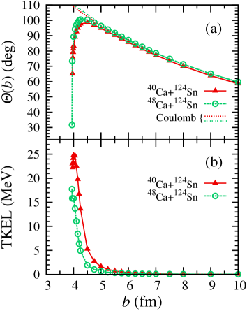
Figure 1: (Color online) Deflection function (a) and total kinetic energy loss (b) as functions of impact parameter $b$ for the reactions of ⁴⁰Ca+¹²⁴Sn at $E_{\mathrm{lab}}=$ 170 MeV and ⁴⁸Ca+¹²⁴Sn at $E_{\mathrm{lab}}=$ 174 MeV. Results for the ⁴⁰Ca+¹²⁴Sn reactions are denoted by red filled triangles connected with solid lines, while results for the ⁴⁸Ca+¹²⁴Sn reactions are denoted by green open circles connected with dashed lines. In (a), we also show deflection functions for the pure Coulomb trajectories by a red dotted line for the ⁴⁰Ca+¹²⁴Sn reactions and by a green two-dot chain line for the ⁴⁸Ca+¹²⁴Sn reactions.

Before showing detailed analyses of transfer reactions, we first present an overview of the reaction dynamics. In Fig. 1, we show the deflection function, $\Theta(b)$, in (a) and the total kinetic energy loss (TKEL) in (b), as functions of impact parameter $b$. Results for the ⁴⁰Ca+¹²⁴Sn reactions are denoted by red filled triangles connected with solid lines, while results for the ⁴⁸Ca+¹²⁴Sn reactions are denoted by green open circles connected with dotted lines. In Fig. 1 (a), we also show deflection functions of the pure Coulomb trajectories by a red dotted line for ⁴⁰Ca+¹²⁴Sn and by a green two-dot chain line for ⁴⁸Ca+¹²⁴Sn.

In practice, the deflection function and the TKEL are calculated in the following way. We denote the center-of-mass coordinate of the PLF (TLF) and the relative coordinate as $\bm{R}_{\mathrm{PLF\,(TLF)}}(t)$ and $\bm{R}(t)=\bm{R}_{\mathrm{PLF}}(t)-\bm{R}_{\mathrm{TLF}}(t)$, respectively. We also denote the mass, charge number, and the reduced mass at the final stage of the calculation as $M_{\mathrm{PLF\,(TLF)}}$, $Z_{\mathrm{PLF\,(TLF)}}$, and $\mu_{f}=M_{\mathrm{PLF}}M_{\mathrm{TLF}}/(M_{\mathrm{PLF}}+M_{\mathrm{TLF}})$. The relative velocity at the final stage of the calculation, $t=t_{f}$, is calculated by $\dot{\bm{R}}(t_{f})=(\bm{R}(t_{f}+\Delta t)-\bm{R}(t_{f}-\Delta t))/2\Delta t$. We evaluate the TKEL by $\mathrm{TKEL}=E_{\mathrm{c.m.}}-\frac{1}{2}\mu_{f}\dot{\bm{R}}(t_{f})^{2}-Z_{\mathrm{PLF}}Z_{\mathrm{TLF}}\,e^{2}/\left|{\bm{R}(t_{f})}\right|$, where $E_{\mathrm{c.m.}}$ is the initial incident energy in the center-of-mass frame. The angle between the vector $\bm{R}(t_{f})$ and the $x$-axis, or the angle between the vector $\dot{\bm{R}}(t_{f})$ and the $x$-axis, provides approximate value of the deflection angle. We estimate the correction for it assuming that both the PLF and the TLF follow the Rutherford trajectory specified by the coordinates and the velocities at the final time, $t_{f}$.

Figure 2: (Color online) Differential cross sections of representative transfer channels as functions of scattering angle in the laboratory frame for the ⁴⁰Ca+¹²⁴Sn reaction at $E_{\mathrm{lab}}=$ 170 MeV. The Coulomb rainbow angle obtained from the TDHF trajectories is denoted by blue solid vertical lines, and is compared with measured differential cross sections, red filled circles, which have been reported in Ref. Corradi(40Ca+124Sn) .

The TKEL increases rapidly as the impact parameter decreases in the region $b<4.5$ fm, where the deflection function, $\Theta(b)$, decreases appreciably by the nuclear attractive interaction. The deflection function shows a maximum at $b\sim$ 4.25 fm and decreases inside this impact parameter. The maximum deflection angle corresponds to the Coulomb rainbow angle, $\theta_{\mathrm{r}}$. It is given by $99^{\circ}$ for ⁴⁰Ca+¹²⁴Sn and $100^{\circ}$ for ⁴⁸Ca+¹²⁴Sn. In Fig. 2, we compare the Coulomb rainbow angle for the ⁴⁰Ca+¹²⁴Sn reaction with measured differential cross sections reported in Ref. Corradi(40Ca+124Sn) . Red filled circles denote measured cross sections and blue solid vertical lines denote the Coulomb rainbow angle in the laboratory frame. As seen from the figure, the peak positions of the measured cross sections roughly coincide with the Coulomb rainbow angle by the TDHF calculation.

Figure 3: (Color online) Snapshots of density distribution of the ⁴⁰Ca+¹²⁴Sn reaction at $E_{\mathrm{lab}}=170$ MeV and $b=$ 3.96 fm, just outside the fusion critical impact parameter.

In Fig. 3, we show snapshots of density distribution for the ⁴⁰Ca+¹²⁴Sn reaction at $b=3.96$ fm, just outside the fusion critical impact parameter, $b_{\mathrm{f}}$. We find a formation of a neck between the projectile and the target during the collision. As will be shown later, several nucleons are exchanged between the projectile and the target at this impact parameter. We find a formation of the neck for the impact parameter region smaller than $b\sim$ 4.25 fm where the TKEL becomes appreciable.

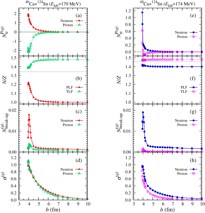
Figure 4: (Color online) Left panels for ⁴⁰Ca+¹²⁴Sn at $E_{\mathrm{lab}}=$ 170 MeV and right panels for ⁴⁸Ca+¹²⁴Sn at $E_{\mathrm{lab}}=$ 174 MeV. (a) and (e): Average number of transferred nucleons from the target to the projectile. (b) and (f): Neutron-to-proton ratios, $N/Z$, of the PLF and the TLF after collision. (c) and (g): Average number of nucleons emitted to the continuum. (d) and (h): Fluctuation of transferred nucleon number. The horizontal axis is the impact parameter $b$. In (b) and (f), the equilibrium $N/Z$ value of the total system is indicated by a horizontal dashed line.

We next consider the average number of transferred nucleons and its fluctuation. We denote the average number of nucleons in the PLF as $N_{\mathrm{PLF}}^{(q)}$ ($q=n$ for neutrons, $p$ for protons), which is calculated from the density distribution at the final stage of the calculation,

$$N_{\mathrm{PLF}}^{(q)}=\int_{\mathrm{around\,PLF}}d\bm{r}\;\;\rho^{(q)}(\bm{r}),$$ (14)

where $\rho^{(q)}(\bm{r})$ is the density distribution of neutrons ($q=n$) or protons ($q=p$). The spatial integration is achieved over a sphere whose center coincides with the center-of-mass of the PLF. The radius of the sphere is taken to be 10 fm. We calculate the average number of nucleons in the TLF in the same way taking the radius of 14 fm for the TLF. We summarize various expressions for the average number and the fluctuation of transferred nucleons in Appendix A.

We denote the neutron (proton) number of the projectile and the target as $N_{\mathrm{P}}^{(q)}$ and $N_{\mathrm{T}}^{(q)}$, respectively. In general, there holds $N_{\mathrm{PLF}}^{(q)}+N_{\mathrm{TLF}}^{(q)}<N_{\mathrm{P}}^{(q)}+N_{\mathrm{T}}^{(q)}$, since some nucleons are emitted to the continuum by the breakup process. As will be shown later, however, the number of nucleons emitted to the continuum is very small in the present calculations. The average number of transferred nucleons from the projectile to the target, $N^{\mathrm{P}(q)}_{\mathrm{tr}}$, is given by

$$N^{\mathrm{P}(q)}_{\mathrm{tr}}=N_{\mathrm{PLF}}^{(q)}-N_{\mathrm{P}}^{(q)}.$$ (15)

Figure 4 shows the average number of transferred nucleons, $N_{\mathrm{tr}}^{\mathrm{P}(q)}$, in (a) and (e), the neutron-to-proton ratios, $N/Z$, of the PLF and the TLF after collision in (b) and (f), the average number of nucleons emitted to the continuum in (c) and (g), and the fluctuation of the transferred nucleon number in (d) and (h), as functions of impact parameter $b$ for ^40, 48Ca+¹²⁴Sn reactions.

In Fig. 4 (a) and (e), the average number of transferred neutrons is shown by filled symbols connected with solid lines, while the average number of transferred protons is shown by open symbols connected with dotted lines. Positive values indicate the increase of the projectile nucleons (transfer from ¹²⁴Sn to ^40, 48Ca) and negative values indicate the decrease (transfer from ^40, 48Ca to ¹²⁴Sn). As seen from Fig. 4 (a) and (e), a large value of average number of transferred nucleons is seen for ⁴⁰Ca+¹²⁴Sn at the impact parameter region close to the fusion critical impact parameter, while the average number of transferred nucleons is small for ⁴⁸Ca+¹²⁴Sn.

We show in Fig. 4 (b) and (f) the neutron-to-proton ratios, $N/Z$, of the PLF and the TLF. For the PLF, it is given by $N_{\mathrm{PLF}}^{(n)}/N_{\mathrm{PLF}}^{(p)}$, and for the TLF by $N_{\mathrm{TLF}}^{(n)}/N_{\mathrm{TLF}}^{(p)}$. Before the collision, the $N/Z$ ratio is given by 1.00 for ⁴⁰Ca, 1.40 for ⁴⁸Ca, and 1.48 for ¹²⁴Sn. The $N/Z$ ratio of the PLF (TLF) is denoted by filled (open) symbols connected with solid (dotted) lines. We also denote the $N/Z$ ratio of the total system by a horizontal dashed line in the figure, 1.34 for ⁴⁰Ca+¹²⁴Sn and 1.46 for ⁴⁸Ca+¹²⁴Sn. We find the nucleons are transferred towards the direction of the charge equilibrium. Namely, protons are transferred from ⁴⁰Ca to ¹²⁴Sn, while neutrons are transferred from ¹²⁴Sn to ⁴⁰Ca in the ⁴⁰Ca+¹²⁴Sn reaction. The $N/Z$ ratios of the projectile and the target do not differ much for ⁴⁸Ca+¹²⁴Sn, and we find a small number of transferred nucleons on average for this reaction. The average number of transferred nucleons decreases rapidly as the impact parameter increases. For the impact parameter region larger than $b\sim 6$ fm, the average number of transferred nucleons almost vanishes.

In Fig. 4 (c) and (g), we show the average number of nucleons emitted to the continuum, $N_{\mathrm{break\mathchar 45\relax up}}^{(q)}\equiv$ $(N_{\mathrm{P}}^{(q)}+N_{\mathrm{T}}^{(q)})-(N_{\mathrm{PLF}}^{(q)}+N_{\mathrm{TLF}}^{(q)})$, during the time evolution. The average number of neutrons (protons) emitted to the continuum is denoted by filled (open) symbols connected with solid (dotted) lines. As seen in the figure, the number of emitted nucleons is very small. The maximum value, about 0.02, is seen at the impact parameter close to the fusion critical impact parameter.

In Fig. 4 (d) and (h), we show the fluctuation of the transferred nucleon number. The expression for the fluctuation is given by Eq. (19). The fluctuation of the transferred neutron (proton) number is denoted by filled (open) symbols connected with solid (dotted) lines. We find the fluctuation decreases as the impact parameter increases. The fluctuation decreases more slowly than the average number of transferred nucleons as a function of impact parameter. We also find the fluctuation of ⁴⁸Ca+¹²⁴Sn is somewhat smaller than but comparable in magnitude to that of ⁴⁰Ca+¹²⁴Sn, although the average number is vanishingly small for ⁴⁸Ca+¹²⁴Sn.

Figure 5: (Color online) Comparison of calculated results for different initial orientations of ¹²⁴Sn in the ⁴⁰Ca+¹²⁴Sn reaction at $E_{\mathrm{lab}}=$ 170 MeV. (a): Average number of transferred nucleons from the target to the projectile. (b): Neutron-to-proton ratios, $N/Z$, of the PLF and the TLF after collision. The horizontal axis is the impact parameter $b$. The initial orientations of ¹²⁴Sn are indicated in legends.

As mentioned in the beginning of this section, we placed the ¹²⁴Sn nucleus which is oblately deformed with $\beta\sim 0.11$ so that the symmetry axis is perpendicular to the reaction plane in the initial configuration. Namely, the symmetry axis of ¹²⁴Sn is set parallel to the $z$-axis. To take fully account of the deformation effect, we should achieve an average over initial orientations of the ¹²⁴Sn. However, since calculations of a number of initial orientations require large computational costs, we do not achieve the orientational average but show results of a specific initial orientation in the present paper. We here briefly discuss the difference of the reaction dynamics depending on the initial orientations.

In Fig. 5, we show the average number of transferred nucleons in (a) and the neutron-to-proton ratios, $N/Z$, of the PLF and the TLF after collision in (b), for three cases of different initial orientations of ¹²⁴Sn in the ⁴⁰Ca+¹²⁴Sn reaction. Red triangles are the same results as those shown in Fig. 4 (a) and (b) where the symmetry axis of ¹²⁴Sn is chosen parallel to the $z$-axis. Green circles correspond to the cases of the symmetry axis set parallel to the $y$-axis (the direction of impact parameter vector). Blue diamonds correspond to the cases of the symmetry axis set parallel to the $x$-axis (the incident direction).

From the figure, we find a rather small difference among three cases of different initial orientations of ¹²⁴Sn. The prominent difference appears only at small impact parameter region. It comes from the difference of the fusion critical impact parameters. Since ¹²⁴Sn is oblately deformed, the Coulomb barrier height is the largest when the symmetry axis of the ¹²⁴Sn is parallel to the $x$-axis (the incident direction).

III.1.2 Transfer probabilities

Figure 6: (Color online) Neutron (left panels) and proton (right panels) transfer probabilities as functions of impact parameter $b$. (a) and (b): Results for the reactions of ⁴⁰Ca+¹²⁴Sn at $E_{\mathrm{lab}}=$ 170 MeV. (c) and (d): Results for the reactions of ⁴⁸Ca+¹²⁴Sn at $E_{\mathrm{lab}}=$ 174 MeV. The positive (negative) number of transferred nucleons represents the number of nucleons added to (removed from) the projectile. Shaded regions at small impact parameter ($b\leq 3.95$ fm for ⁴⁰Ca+¹²⁴Sn and $b\leq 3.93$ fm for ⁴⁸Ca+¹²⁴Sn) correspond to the fusion reactions.

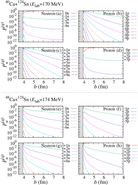
Figure 7: (Color online) Transfer probabilities in Fig. 6 are shown in logarithmic scale. Nucleon transfer probabilities opposite to the direction of the charge equilibrium, which are not included in Fig. 6, are shown as well.

We next show transfer probabilities as functions of impact parameter which are obtained from the final wave functions using the number projection procedure of Eq. (LABEL:P_n_projection). The nucleon transfer probabilities, $P_{n}^{(q)}(b)$, are shown in Fig. 6 (linear scale) and in Fig. 7 (logarithmic scale). Top panels of Fig. 6 ((a) and (b)) and top panels of Fig. 7 ((a), (b), (c), and (d)) show results of the ⁴⁰Ca+¹²⁴Sn reaction, while lower panels of Fig. 6 ((c) and (d)) and lower panels of Fig. 7 ((e), (f), (g), and (h)) show results of the ⁴⁸Ca+¹²⁴Sn reaction. In these figures, shaded regions at small impact parameter ($b\leq 3.95$ fm for ⁴⁰Ca+¹²⁴Sn and $b\leq 3.93$ fm for ⁴⁸Ca+¹²⁴Sn) correspond to the fusion reactions. The positive (negative) number of transferred nucleons represents the number of nucleons added to (removed from) the projectile.

From the figure, we find that probabilities of single-nucleon transfer (green dashed lines) extend to a large impact parameter region. As the number of transferred nucleons increases, the reaction probability is sizable only at a small impact parameter region, close to the fusion critical impact parameter.

The directions of the transfer processes are the same as those we observed in the average number of transferred nucleons in Fig. 4 (a) and (e). Namely, in the case of ⁴⁰Ca+¹²⁴Sn (Fig. 6 (a) and (b)), protons are transferred from ⁴⁰Ca to ¹²⁴Sn and neutrons are transferred from ¹²⁴Sn to ⁴⁰Ca, the directions towards the charge equilibrium. We note that the transfer probabilities towards the opposite directions, proton transfer from ¹²⁴Sn to ⁴⁰Ca and neutron transfer from ⁴⁰Ca to ¹²⁴Sn, are very small and are hardly seen in the linear scale figure (Fig. 6 (a) and (b)). In the logarithmic scale (Fig. 7 (a), (b), (c), and (d)), we find the transfer probabilities towards the opposite direction to the charge equilibrium are smaller than those towards the charge equilibrium by at least an order of magnitude. In the case of ⁴⁸Ca+¹²⁴Sn reaction (Fig. 6 (c) and (d), Fig. 7 (e), (f), (g), and (h)), the transfer probabilities towards both directions are the same order of magnitude. This is consistent with the fact that the average number of transferred nucleons is very small as shown in Fig. 4 (e).

III.1.3 Transfer cross sections

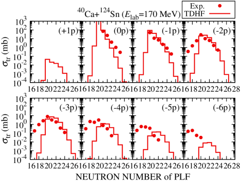
Figure 8: (Color online) Cross sections for transfer channels classified according to the change of the proton number of the PLF from ⁴⁰Ca, as functions of neutron number of the PLF for the ⁴⁰Ca+¹²⁴Sn reaction at $E_{\mathrm{lab}}=$ 170 MeV. Red filled circles denote measured cross sections and red solid lines denote results of the TDHF calculations. The number of transferred protons is indicated as ($x$p) ($-6\leq x\leq+1$). The measured cross sections have been reported in Ref. Corradi(40Ca+124Sn) .

Integrating the transfer probabilities over impact parameter, we obtain transfer cross sections. The results are shown in Fig. 8 for ⁴⁰Ca+¹²⁴Sn and in Fig. 9 for ⁴⁸Ca+¹²⁴Sn.

We first examine the ⁴⁰Ca+¹²⁴Sn reaction. Figure 8 shows the transfer cross sections classified according to the change of the proton number of the PLF from ⁴⁰Ca, as functions of neutron number of the PLF. Red filled circles denote measured cross sections and red solid lines denote results of the TDHF calculations. We show transfer cross sections of one proton added to ($+1$p) through six proton removed from ($-6$p) ⁴⁰Ca.

We find the experimental data are reasonably reproduced by the TDHF calculations for cross sections without proton transfer shown in ($0$p) panel, although the cross sections are somewhat underestimated as the number of transferred neutrons increases. Zero- to four-neutron pick-up channels shown in ($-1$p), ($-2$p), and ($-3$p) panels are also reproduced reasonably. The calculated cross sections towards the direction opposite to the charge equilibrium are small, consistent with the observation in transfer probabilities shown in Fig. 7 (a) and (d).

As the number of transferred protons increases, there appear some discrepancies between the TDHF calculations and the measurements. When more than one protons are transferred, the TDHF calculation underestimates measured cross sections of neutron removal channels ($N<20$). For five- and six-proton removal channels, ($-5$p) and ($-6$p), the TDHF cross sections become too small compared with the measurements. We also find a shift of the peak position towards the larger neutron number.

In Ref. Corradi(40Ca+124Sn) , cross sections calculated by the GRAZING code GRAZING were compared with the measurements. In the GRAZING calculation, a similar discrepancy was observed. As the origin of the discrepancy, the significance of the evaporation effects has been mentioned Corradi(40Ca+124Sn) . We will compare our results with those of the GRAZING calculations in Sec. IV.

We note that particle evaporation processes are not taken into account sufficiently in the present calculation. In Fig. 1 (b), we find the TKEL of as large as 25 MeV at a small impact parameter region where appreciable multinucleon transfer probabilities are found. The amount of the TKEL is sufficiently large to emit some nucleons to the continuum. However, as we saw in Fig. 4 (c), the average number of nucleons emitted to the continuum is very small, the maximum value is only 0.02. Although we have not yet estimated the number of evaporated nucleons, the inclusion of the evaporation processes is expected to reduce the discrepancy as follows. Neutron evaporation processes will shift the peak position of the transfer cross sections towards the smaller neutron number (left direction in Fig. 8). We may also expect that proton evaporation processes will shift cross section of $n$-proton removal channels to ($n+1$)-proton removal channels.

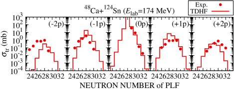
Figure 9: (Color online) Cross sections for transfer channels classified according to the change of the proton number of the PLF from ⁴⁸Ca, as functions of neutron number of the PLF for the ⁴⁸Ca+¹²⁴Sn reaction at $E_{\mathrm{lab}}=$ 174 MeV. Red filled circles denote measured cross sections and red solid lines denote results of the TDHF calculations. The number of transferred protons is indicated as ($x$p) ($-2\leq x\leq+2$). The measured cross sections have been reported in Ref. Corradi(48Ca+124Sn) .

Figure 9 shows transfer cross sections of ⁴⁸Ca+¹²⁴Sn reaction. The cross sections obtained from the TDHF calculations are in good agreement with the experimental data for zero- and one-proton transfer channels, ($0$p) and ($\pm 1$p). For two-proton transfer channels ($\pm 2$p), however, our TDHF calculations underestimate the cross sections. In the case of two-proton removal channels ($-2$p), the peak position shifts towards larger neutron number, while in the case of two-proton pickup channels ($+2$p), the peak position shifts towards smaller neutron number. The underestimation in the ($-2$p) channels may be remedied by taking into account the neutron evaporation processes as in the case of ⁴⁰Ca+¹²⁴Sn reaction. However, the underestimation in the ($+2$p) channels may not. A similar discrepancy was reported in the GRAZING calculation Corradi(48Ca+124Sn) . In Ref. Corradi(48Ca+124Sn) , more complex mechanisms such as neutron-proton pair transfer and/or $\alpha$-cluster transfer have been advocated for the origin of the discrepancy.

III.2 ⁴⁰Ca+²⁰⁸Pb reaction

In this subsection, we present results for the reactions of ⁴⁰Ca+²⁰⁸Pb at $E_{\mathrm{lab}}=$ 235 and 249 MeV ($E_{\mathrm{c.m.}}\simeq$ 197.1 and 208.8 MeV), for which measurements have been reported in Ref. Szilner(40Ca+208Pb)2 . This system has $Z_{\mathrm{P}}Z_{\mathrm{T}}=$ 1640, close to 1600. Therefore, we expect an appearance of the indication of the fusion-hindrance. We estimate the Coulomb barrier height of this system using the frozen-density approximation, giving $V_{\mathrm{B}}\approx$ 178.4 MeV. Since the collision energies are higher than the barrier height, we find finite values of the fusion critical impact parameter $b_{\mathrm{f}}$, as in the ^40, 48Ca+¹²⁴Sn reactions. They are given by $b_{\mathrm{f}}=3.81$ and 4.55 fm at $E_{\mathrm{lab}}=$ 235 and 249 MeV, respectively.

III.2.1 Overview of the reactions

We first present an overview of the reaction dynamics. In Fig. 10, we show the deflection function in (a) and the TKEL in (b), as functions of impact parameter. Results for the reaction at $E_{\mathrm{lab}}=$ 235 MeV are denoted by red filled triangles connected with solid lines, while results for the reaction at $E_{\mathrm{lab}}=$ 249 MeV are denoted by green open circles connected with dotted lines. In Fig. 10 (a), we also show deflection functions for the pure Coulomb trajectories at $E_{\mathrm{lab}}=$ 235 MeV by a red dotted line and at $E_{\mathrm{lab}}=$ 249 MeV by a green two-dot chain line. In this system, we find an increase of the TKEL up to around 50 MeV and 60 MeV for the incident energies of 235 MeV and 249 MeV, respectively. This maximum value of TKEL is about a factor of two larger than the case of ^40, 48Ca+¹²⁴Sn reactions. We find the difference of the TKEL between these systems, ⁴⁰Ca+²⁰⁸Pb and ^40, 48Ca+¹²⁴Sn, comes from properties of the neck whose formation is observed when the TKEL becomes substantial.

Figure 10: (Color online) Deflection function (a) and total kinetic energy loss (b) as functions of impact parameter $b$ for the reactions of ⁴⁰Ca+²⁰⁸Pb at $E_{\mathrm{lab}}=$ 235 and 249 MeV. Results for the reactions at $E_{\mathrm{lab}}=$ 235 MeV are denoted by red filled triangles connected with solid lines, while results for the reactions at $E_{\mathrm{lab}}=$ 249 MeV are denoted by green open circles connected with dashed lines. In (a), we also show deflection functions for the pure Coulomb trajectories at $E_{\mathrm{lab}}=$ 235 MeV by a red dotted line and at $E_{\mathrm{lab}}=$ 249 MeV by a green two-dot chain line.

Figure 11: (Color online) Snapshots of density distribution of the ⁴⁰Ca+²⁰⁸Pb reaction at $E_{\mathrm{lab}}=$ 249 MeV and $b=$ 4.56 fm, just outside the fusion critical impact parameter.

In Fig. 11, we show snapshots of density distribution for the ⁴⁰Ca+²⁰⁸Pb reaction at $E_{\mathrm{lab}}=$ 249 MeV and $b=4.56$ fm, just outside the fusion critical impact parameter. The neck is seen to be formed solidly for a long period from $t=$ 200 fm/c to 3000 fm/c. This process may be regarded as a quasi-fission. As will be shown below, a number of nucleons are transferred from ²⁰⁸Pb to ⁴⁰Ca at this impact parameter.

Figure 12: (Color online) Differential cross sections of representative transfer channels as functions of scattering angle in the center-of-mass frame for the ⁴⁰Ca+²⁰⁸Pb reactions at $E_{\mathrm{lab}}=$ 235 and 249 MeV. The Coulomb rainbow angle obtained from the TDHF trajectories is denoted by red solid (green dotted) vertical lines for $E_{\mathrm{lab}}=$ 235 (249) MeV. They are compared with measured differential cross sections, red filled triangles (green open circles) for $E_{\mathrm{lab}}=$ 235 (249) MeV, which have been reported in Ref. Szilner(40Ca+208Pb)2 .

The period of the neck formation is longer in the present ⁴⁰Ca+²⁰⁸Pb case than that in the ^40, 48Ca+¹²⁴Sn cases. We find the neck formation for the periods of 1000-3000 fm/c and more for the present system depending on the impact parameter, while it is at most 300 fm/c in the ^40, 48Ca+¹²⁴Sn systems. We consider this difference is related to the different $Z_{\mathrm{P}}Z_{\mathrm{T}}$ values of these systems. Since $Z_{\mathrm{P}}Z_{\mathrm{T}}\gtrsim$ 1600 in the present system, fusion reactions are hindered by the quasi-fission process. Namely, there appears a certain impact parameter region in which binary final fragments are produced after a rather solid neck formation during the collision.

The Coulomb rainbow angle is $\theta_{\mathrm{r}}\simeq$ 99^∘ for the reaction at $E_{\mathrm{lab}}=$ 235 MeV and $\theta_{\mathrm{r}}\simeq$ 86^∘ for the reaction at $E_{\mathrm{lab}}=$ 249 MeV, respectively. The deflection function becomes negative at the small impact parameter region, reaching $-200^{\circ}$ just outside $b_{\mathrm{f}}$. In Fig. 12, we compare the Coulomb rainbow angles for the ⁴⁰Ca+²⁰⁸Pb reactions at $E_{\mathrm{lab}}=$ 235 and 249 MeV with measured differential cross sections which have been reported in Ref. Szilner(40Ca+208Pb)2 . Red filled triangles denote measured cross sections for $E_{\mathrm{lab}}=$ 235 MeV, while green open circles denote those for $E_{\mathrm{lab}}=$ 249 MeV. The Coulomb rainbow angle obtained from the TDHF trajectories is denoted by red solid (green dotted) vertical lines for $E_{\mathrm{lab}}=$ 235 (249) MeV. We find the peak positions of measured angular distributions are reasonably reproduced by the TDHF calculation.

Figure 13: (Color online) The ⁴⁰Ca+²⁰⁸Pb reactions at $E_{\mathrm{lab}}=$ 235 and 249 MeV. (a): Average number of transferred nucleons from the target to the projectile. (b): Neutron-to-proton ratios, $N/Z$, of the PLF and the TLF after collision. (c): Average number of nucleons emitted to the continuum. (d): Fluctuation of transferred nucleon number. The horizontal axis is the impact parameter $b$. Results for the reactions at $E_{\mathrm{lab}}=$ 235 MeV are denoted by triangles, while results for the reactions at $E_{\mathrm{lab}}=$ 249 MeV are denoted by circles. In (b), the equilibrium $N/Z$ value of the total system, 1.43, is indicated by a horizontal dashed line.

Figure 13 shows the average number of transferred nucleons in (a), the $N/Z$ ratios of the PLF and the TLF in (b), the average number of nucleons emitted to the continuum in (c), and the fluctuation of the transferred nucleon number in (d), as functions of impact parameter. In each panel, triangles represent results for $E_{\mathrm{lab}}=$ 235 MeV and circles represent results for $E_{\mathrm{lab}}=$ 249 MeV.

In Fig. 13 (a), the average number of transferred neutrons is shown by filled symbols connected with solid lines, while the average number of transferred protons is shown by open symbols connected with dotted lines. Positive values indicate the increase of the projectile nucleons (transfer from ²⁰⁸Pb to ⁴⁰Ca) and negative values indicate the decrease (transfer from ⁴⁰Ca to ²⁰⁸Pb). As seen from the figure, the average number of transferred protons shows a minimum at a certain impact parameter ($b=$ 4.0 fm for $E_{\mathrm{lab}}=$ 235 MeV and $b=$ 5.0 fm for $E_{\mathrm{lab}}=$ 249 MeV). Outside this impact parameter, the nucleon transfer process proceeds towards the direction of the charge equilibrium of the projectile and the target. Inside this impact parameter, neutrons are still transferred towards the same direction. However, the number of transferred protons decreases and becomes positive, which corresponds to the transfer from ²⁰⁸Pb to ⁴⁰Ca.

At first sight, the direction of the proton transfer at small impact parameter region is opposite to the direction of the charge equilibrium. However, it is not the case as can be understood from Fig. 13 (b) which shows the neutron-to-proton ratios, $N/Z$, of the PLF (filled symbols connected with solid lines) and the TLF (open symbols connected with dotted lines), which are obtained from the average numbers of the nucleons shown in Fig. 13 (a). Before collision, the $N/Z$ ratio is given by 1.00 for ⁴⁰Ca and 1.54 for ²⁰⁸Pb. In Fig. 13 (b), the $N/Z$ ratio of the total system, 1.43, is shown by a horizontal dashed line. As seen from the figure, the nucleon transfer processes proceed towards the direction of the charge equilibrium for both the PLF and the TLF at all impact parameter region outside the fusion critical impact parameter. Even though the average number of transferred protons shows complex behavior at small impact parameter region, the $N/Z$ ratios of the PLF and the TLF monotonically approach to the fully equilibrated value of 1.43 as the impact parameter decreases.

The change of sign of the average number of transferred protons at small impact parameter region is found to be related to the formation of a rather solid neck. When the neck is broken, we find that most part of the neck is absorbed by the lighter fragment (cf. Fig. 11). Since the neck is composed of both neutrons and protons, the absorption of the nucleons in the neck region results in the increase of average number of nucleons in the PLF for both neutrons and protons (see Fig. 13 (a)).

In Fig. 13 (c), we show the average number of nucleons emitted to the continuum during the time evolution. The average number of neutrons (protons) emitted to the continuum is denoted by filled (open) symbols connected with solid (dotted) lines. We count it by subtracting the number of nucleons inside a sphere of 14 fm for the TLF and that inside a sphere of 10 fm for the PLF from the total number of nucleons, 248. The average number of emitted nucleons is again very small, at most 0.1 around the fusion critical impact parameter.

In Fig. 13 (d), we show the fluctuation of the transferred nucleon number. The fluctuation of transferred neutron (proton) number is denoted by filled (open) symbols connected with solid (dotted) lines. The fluctuation increases monotonically as the impact parameter decreases, reaching the maximum value roughly 1.3 around the fusion critical impact parameter. Although the average number of transferred protons is small at the small impact parameter region, the fluctuation of transferred proton number has value as large as that of neutrons. This fact indicates that single-particle wave functions of protons are exchanged actively between the projectile and the target, although the number of transferred protons is small on average.

III.2.2 Transfer probabilities

Figure 14: (Color online) Neutron and proton transfer probabilities as functions of impact parameter $b$ for the ⁴⁰Ca+²⁰⁸Pb reactions. (a), (b), (c), and (d): Results at $E_{\mathrm{lab}}=$ 235 MeV. (e), (f), (g), and (h): Results at $E_{\mathrm{lab}}=$ 249 MeV. The positive (negative) number of transferred nucleons represents the number of nucleons added to (removed from) the projectile. Note that horizontal scales are different between the left and the right panels. Shaded regions at small impact parameter ($b\leq 3.81$ fm for $E_{\mathrm{lab}}=$ 235 MeV and $b\leq 4.55$ fm for $E_{\mathrm{lab}}=$ 249 MeV) correspond to the fusion reactions.

The nucleon transfer probabilities, $P_{n}^{(q)}(b)$, are shown in Fig. 14. Top panels ((a), (b), (c), and (d)) show results at $E_{\mathrm{lab}}=$ 235 MeV, while lower panels ((e), (f), (g), and (h)) show results at $E_{\mathrm{lab}}=$ 249 MeV. In the figure, shaded regions at small impact parameter ($b\leq 3.81$ fm for $E_{\mathrm{lab}}=$ 235 MeV and $b\leq 4.55$ fm for $E_{\mathrm{lab}}=$ 249 MeV) correspond to the fusion reactions. The positive (negative) number of transferred nucleons represents the number of nucleons added to (removed from) the projectile. In the left panels ((a), (c), (e), and (g)), we show transfer probabilities, ($0$n) to ($+4$n) for neutrons and ($0$p) to ($-4$p) for protons. In the right panels ((b), (d), (f), and (h)), we show transfer probabilities, ($+1$n) to ($+9$n) for neutrons and ($-4$p) to ($+4$p) for protons, at small impact parameter regions just outside the fusion critical impact parameter. Probabilities of neutron transfer from ⁴⁰Ca to ²⁰⁸Pb are very small and are not shown.

As in the case of ^40, 48Ca+¹²⁴Sn reactions, we find that probabilities of single-nucleon transfer (green dashed lines) extend to a large impact parameter region. Reaction probabilities for multinucleon transfer processes become appreciable at a small impact parameter region close to the fusion critical impact parameter. The transfer probabilities towards the charge equilibrium are large in most cases. At a small impact parameter region just outside the fusion critical impact parameter, however, we find substantial probabilities for the proton transfer processes opposite to the charge equilibrium as seen in the right panels of Fig. 14 ((b), (d), (f), and (h)). This is related to the increase of the average number of transferred protons at small impact parameter region which was seen in Fig. 13 (a).

III.2.3 Transfer cross sections

Figure 15: (Color online) Transfer cross sections for the ⁴⁰Ca+²⁰⁸Pb reactions at $E_{\mathrm{lab}}=$ 235 and 249 MeV. Red filled triangles (green open circles) denote measured cross sections at $E_{\mathrm{lab}}=$ 235 (249) MeV. Red solid (green dotted) lines denote results of the TDHF calculations at $E_{\mathrm{lab}}=$ 235 (249) MeV. The number of transferred protons (positive number for the transfer from ²⁰⁸Pb to ⁴⁰Ca) is indicated as ($x$p) ($-6\leq x\leq+5$). The measured cross sections have been reported in Ref. Szilner(40Ca+208Pb)2

Figure 16: (Color online) The same transfer cross sections for the ⁴⁰Ca+²⁰⁸Pb reactions as those in Fig. 14. The number of transferred neutrons is indicated as ($x$n) ($-5\leq x\leq+9$).

We show transfer cross sections in Figs. 15 and 16. Each panel of Fig. 15 shows cross sections classified according to the change of the proton number of the PLF from ⁴⁰Ca which is indicated by ($x$p) ($-6\leq x\leq+5$), as functions of neutron number of the PLF. Each panel of Fig. 16 shows cross sections classified according to the change of the neutron number of the PLF from ⁴⁰Ca which is indicated by ($x$n) ($-5\leq x\leq+9$), as functions of proton number of the PLF. Red filled triangles denote measured cross sections for $E_{\mathrm{lab}}=$ 235 MeV, while green open circles denote those for $E_{\mathrm{lab}}=$ 249 MeV. Cross sections calculated by the TDHF are denoted by red solid (green dotted) lines for $E_{\mathrm{lab}}=$ 235 (249) MeV. As seen in the average number of transferred nucleons in Fig. 13 (a) and in the transfer probabilities in Fig. 14, the transfer cross sections towards the direction of the charge equilibrium dominate.

In ($0$p) and ($-1$p) panels of Fig. 15, the TDHF calculation is seen to reproduce the measured cross sections up to six-neutron transfer. As the number of transferred protons increases, ($-2$p) to ($-6$p), the cross sections in the TDHF calculation show a maximum at a neutron number more than that of ⁴⁰Ca. Compared with measured cross sections, the TDHF results shift towards larger values of neutron number. This behavior is similar to the case of ⁴⁰Ca+¹²⁴Sn reaction. Looking at the transfer cross sections for a fixed number of transferred neutrons in Fig. 16, the TDHF calculations reproduce ($+1$n) and ($+2$n) panels rather well.

As seen in Fig. 15, the TDHF calculations provide substantial cross sections for proton pickup reactions, ($+1$p) to ($+5$p), which is the transfer towards the opposite direction of the charge equilibrium expected from the initial $N/Z$ ratios. The cross sections show a peak around the neutron number 28. The TDHF calculations also provide substantial cross sections for many neutron pickup reactions (see bottom row of Fig. 16). The cross sections show a peak around the proton number 20. These cross sections come from an impact parameter region close to the fusion critical impact parameter. As seen in Fig. 13 (a), a large average number of transferred neutrons up to 10 is seen while the average number of transferred protons has small value. We note that the collision close to the fusion critical impact parameter accompanies large TKEL, and should suffer substantial evaporation effects which are not treated in the present analyses.

The TDHF calculation systematically underestimates the cross section of neutron transfer processes from ⁴⁰Ca to ²⁰⁸Pb, ($-1$n) to ($-5$n) (see top row of Fig. 16). Although these processes are against the charge equilibrium, substantial cross sections are observed experimentally. In the TDHF calculation, cross sections of neutron transfer channels opposite to the charge equilibrium are several orders of magnitude smaller than the measurements. In Ref. Szilner(40Ca+208Pb)2 , it has been argued that the neutron evaporation after collision is responsible for these channels.

III.3 ⁵⁸Ni+²⁰⁸Pb reaction

As a final case, we present results for the ⁵⁸Ni+²⁰⁸Pb reaction at $E_{\mathrm{lab}}=$ 328.4 MeV ($E_{\mathrm{c.m.}}\simeq$ 256.8 MeV), for which measurements are reported in Ref. Corradi(58Ni+208Pb) . Since this system has $Z_{\mathrm{P}}Z_{\mathrm{T}}$ = 2296 exceeding the critical value 1600, we may expect an appearance of the quasi-fission process at a small impact parameter region. Using the frozen-density approximation, the Coulomb barrier height is estimated to be $V_{\mathrm{B}}\approx$ 247.6 MeV, which is lower than the center-of-mass energy. We find the fusion critical impact parameter $b_{\mathrm{f}}$ given by 1.38 fm for this reaction. To decide whether the nucleus once gets fused eventually decays into fragments or not, we continue to calculate the time evolution up to 4000 fm/c after two nuclei touches. If the fused system keeps compact form for this period, we regard the process as fusion.

III.3.1 Overview of the reaction

Figure 17: (Color online) Deflection function (a) and total kinetic energy loss (b) as functions of impact parameter $b$ for the reactions of ⁵⁸Ni+²⁰⁸Pb at $E_{\mathrm{lab}}=$ 328.4 MeV. In (a), we show a deflection function for the pure Coulomb trajectory by a dotted line.

Figure 18: (Color online) Differential cross sections of representative transfer channels as functions of scattering angle in the center-of-mass frame for the ⁵⁸Ni+²⁰⁸Pb reaction at $E_{\mathrm{lab}}=$ 328.4 MeV. The Coulomb rainbow angle obtained from the TDHF trajectories is denoted by blue solid vertical lines, and is compared with measured differential cross sections, red filled circles, which have been reported in Ref. Corradi(58Ni+208Pb) .

We first present an overview of the reaction dynamics. In Fig. 17, we show the deflection function in (a) and the TKEL in (b), as functions of impact parameter. In (a), we also show a deflection function for the pure Coulomb trajectory by a dotted line. The Coulomb rainbow occurs at the impact parameter of 2.5 fm and the rainbow angle is $\theta_{\mathrm{r}}\simeq 121^{\circ}$. In Fig. 18, we compare the Coulomb rainbow angle with measured differential cross sections which have been reported in Ref. Corradi(58Ni+208Pb) . Red filled circles denote measured cross sections and blue solid vertical lines denote the Coulomb rainbow angle. From the figure, we find the measured differential cross sections show rather flat distributions compared with lighter systems. This may be related to a rather small curvature of the deflection function around the Coulomb rainbow angle obtained from the TDHF trajectories as seen in Fig. 17 (a).

The TKEL shows a behavior different from lighter systems. The maximum TKEL is about 50-60 MeV, similar to the value observed in ⁴⁰Ca+²⁰⁸Pb reaction. However, there is a large impact parameter region, from 1.39 fm to 2.75 fm, in which the TKEL takes approximately the same value.

Figure 19: (Color online) Snapshots of density distribution of the ⁵⁸Ni+²⁰⁸Pb reaction at $E_{\mathrm{lab}}=$ 328.4 MeV and $b=$ 1.39 fm, just outside the fusion critical impact parameter.

In Fig. 19, we show snapshots of density distribution for the ⁵⁸Ni+²⁰⁸Pb reaction at the impact parameter of 1.39 fm, just outside the fusion critical impact parameter. In the course of the collision, colliding nuclei form a rather thick neck and excurse for a long period connected by the neck. We find the two nuclei are connected for a period as long as 3600 fm/c. For collisions in the impact parameter region where the TKEL takes values around 50-60 MeV, we find a formation of a similar thick neck which persists rather long period. These reactions are considered to correspond to the quasi-fission.

Figure 20: (Color online) The ⁵⁸Ni+²⁰⁸Pb reaction at $E_{\mathrm{lab}}=$ 328.4 MeV. (a): Average number of transferred nucleons from the target to the projectile. (b): Neutron-to-proton ratios, $N/Z$, of the PLF and the TLF after collision. (c): Average number of nucleons emitted to the continuum. (d): Fluctuation of transferred nucleon number. The horizontal axis is the impact parameter $b$. In (b), the equilibrium $N/Z$ value of the total system, 1.42, is indicated by a horizontal dashed line.

Figure 20 shows the average number of transferred nucleons in (a), the $N/Z$ ratios of the PLF and the TLF in (b), the average number of nucleons emitted to the continuum in (c), and the fluctuation of the transferred nucleons in (d), as functions of impact parameter.

In Fig. 20 (a), the average number of transferred neutrons is shown by red filled circles connected with solid lines, while the average number of transferred protons is shown by green open circles connected with dotted lines. Positive numbers indicate the increase of the projectile nucleons (transfer from ²⁰⁸Pb to ⁵⁸Ni) and negative numbers indicate the decrease (transfer from ⁵⁸Ni to ²⁰⁸Pb). From the figure, we find the average number of transferred protons shows a minimum at $b=$ 2.75 fm. We note that this value coincides with the impact parameter inside which the TKEL becomes almost constant in Fig. 17 (b). A similar minimum was also seen in the ⁴⁰Ca+²⁰⁸Pb case, as shown in Fig. 13 (a). Outside this impact parameter, nucleons are transferred towards the direction of the charge equilibrium expected from the initial $N/Z$ ratios. In the impact parameter region, 1.55 fm $\leq b\leq$ 2.75 fm, the average number of transferred nucleons increases as the impact parameter decreases for both neutrons and protons. A similar behavior was also seen in ⁴⁰Ca+²⁰⁸Pb reaction as in Fig. 13 (a).

At the impact parameter region $b<$ 1.85 fm, the average number of transferred protons becomes positive, opposite to the direction of the charge equilibrium of the initial system. However, the nucleon transfer still proceeds towards the charge equilibrium of both the PLF and the TLF after the collision. This is clearly seen in Fig. 20 (b) which shows the $N/Z$ ratios of the PLF and the TLF after collision. The $N/Z$ ratio of the PLF (TLF) is denoted by red filled (green open) circles connected with solid (dotted) lines. As seen from the figure, the $N/Z$ ratios of both the PLF and the TLF become closer to the $N/Z$ ratio of the total system, 1.42, which is represented by a horizontal dashed line.

As mentioned in the case of ⁴⁰Ca+²⁰⁸Pb reactions, the change in the average number of transferred protons across the impact parameter $b\sim 3$ fm is related to the formation of the neck. Outside $b\sim 3$ fm, the neck is not formed and two nuclei are separated even at the closest approach. In such case, nucleons are transferred towards the direction of the charge equilibrium expected from the initial $N/Z$ ratios. Inside $b\sim 3$ fm, the neck is formed between two nuclei. Then the transfer of nucleons proceeds in two steps. Before the formation of the neck, the transfer of nucleons proceeds towards the charge equilibrium of the initial system in the same way as that in $b>3$ fm. After the formation of the neck, an exchange of a large number of nucleons occurs at the time of the breaking of the neck. Depending on the position of the neck breaking, the transfer of nucleons is expected in either directions, from the target to the projectile or the reverse. Since the neck is formed with both protons and neutrons, the nucleon transfer in the neck breaking process accompanies both protons and neutrons in the same direction.

Looking at Fig. 20 (a), we find the increase of the average numbers of transferred nucleons of both neutrons and protons as the impact parameter decreases below $b=2.75$ fm. This indicates that the neck is broken at the position close to the target. Both protons and neutrons in the neck region are absorbed by the projectile. This mechanism explains the reason why the number of transferred protons increases as the impact parameter decreases in Fig. 20 (a). This transfer process associated with the neck breaking was also seen in the ^40, 48Ca+¹²⁴Sn and the ⁴⁰Ca+²⁰⁸Pb reactions.

At very small impact parameter region, 1.40 fm $\leq b\leq$ 1.50 fm, the average number of transferred neutrons shows a large fluctuation. The average number of transferred protons also shows the fluctuation, correlated with that of neutrons. These fluctuations occur by changes of the breaking point of the neck. When the neck is broken close to the target, a large number of nucleons are transferred from the target to the projectile, while the neck is broken at a midpoint between the projectile and the target, the number of transferred nucleons becomes small.

Figure 20 (c) shows the average number of nucleons emitted to the continuum during the time evolution. The average number of neutrons (protons) emitted to the continuum is denoted by red filled (green open) circles connected with solid (dotted) lines. As in other systems, we calculate it by subtracting the average number of nucleons inside a sphere of 14 fm for the TLF and that inside a sphere of 10 fm for the PLF from the total number of nucleons, 266. Again the number is rather small, about 0.12 at the maximum.

Figure 20 (d) shows the fluctuation of the transferred nucleon number. The fluctuation of transferred neutron (proton) number is denoted by red filled (green open) circles connected with solid (dotted) lines. They show a different behavior across the impact parameter around 3 fm, indicating a qualitative change of the dynamics. Outside this impact parameter where protons and neutrons are transferred in different directions, the fluctuation of transferred neutron number is larger than that of protons. Inside this impact parameter, although the average number of transferred neutrons is much larger than that of protons, the fluctuation is almost the same. This indicates that although the average number of transferred protons is small, there is a strong mixture of single-particle orbitals of protons due to the formation and breaking of the neck.

III.3.2 Transfer probabilities

Figure 21: (Color online) Neutron and proton transfer probabilities as functions of impact parameter $b$ for the reactions of ⁵⁸Ni+²⁰⁸Pb at $E_{\mathrm{lab}}=$ 328.4 MeV. Figure (a) and (b) show probabilities of neutrons, while figure (c) and (d) show those of protons. The positive (negative) number of transferred nucleons represents the number of nucleons added to (removed from) the projectile. Note that horizontal scales are different between the left and the right panels. A shaded region at small impact parameter ($b\leq 1.38$ fm) corresponds to the fusion reactions.

We next show transfer probabilities of the ⁵⁸Ni+²⁰⁸Pb reaction as functions of impact parameter, which are shown in Fig. 21. The small impact parameter region ($b\leq 1.38$ fm) corresponding to the fusion reaction are shaded. The positive (negative) number of the transferred nucleons represents the number of nucleons added to (removed from) the projectile. The upper (lower) panels show neutron (proton) transfer probabilities for each transfer channel. In the left panels ((a) and (c)), we show transfer probabilities, ($0$n) to ($+6$n) for neutrons and ($0$p) to ($-4$p) for protons. They correspond to the transfer processes towards the charge equilibrium of the initial system. In the right panels ((b) and (d)), we show transfer probabilities, ($+7$n) to ($+13$n) for neutrons and ($+1$p) to ($+5$p) for protons, which dominate in the small impact parameter region, $b\leq$ 2.75 fm. Probabilities of neutron transfer from ⁵⁸Ni to ²⁰⁸Pb are very small and are not shown.

In contrast to the previous cases of ^40, 48Ca+¹²⁴Sn and ⁴⁰Ca+²⁰⁸Pb, probabilities of transfer processes involving more than 6 neutrons are seen in rather wide impact parameter region, 1.39 fm $\leq b\leq$ 2.75 fm, where the formation of the thick neck is observed. In Fig. 17 (b), a large value of TKEL was also seen in the impact parameter region of $b<3$ fm, indicating the significance of the evaporation effects.

Figure 22: (Color online) Transfer cross sections for the ⁵⁸Ni+²⁰⁸Pb reaction at $E_{\mathrm{lab}}=$ 328.4 MeV. Red filled circles denote measured cross sections and red solid lines denote results of the TDHF calculations. The number of transferred protons (positive number for the transfer from ²⁰⁸Pb to ⁵⁸Ni) is indicated as ($x$p) ($-6\leq x\leq+5$). The measured cross sections have been reported in Ref. Corradi(58Ni+208Pb) .

As in previous cases, probabilities of the processes accompanying small number of exchanged nucleons show large spatial tail. The transfer probabilities for channels towards the charge equilibrium are large in most cases. The zero-proton transfer probability ($0$p, red solid line) in Fig. 21 (c) decreases as the impact parameter decreases, shows minimum at $b\sim 3$ fm, and again increases at smaller impact parameter region. This behavior is consistent with the behavior of the average number of transferred protons seen in Fig. 20 (a). Although neutron transfer probabilities to the direction opposite to the charge equilibrium of the initial system are vanishingly small, we find appreciable probabilities of proton transfer opposite to the charge equilibrium of the initial system, as is seen from Fig. 21 (d). This feature is again consistent with the behavior of the average number of transferred protons shown in Fig. 20 (a).

III.3.3 Transfer cross sections

Figure 23: (Color online) The same transfer cross sections for the ⁵⁸Ni+²⁰⁸Pb reaction as those in Fig. 21. The number of transferred neutrons is indicated as ($x$n) ($-4\leq x\leq+10$).

We show transfer cross sections in Fig. 22 and Fig. 23. Each panel of Fig. 22 shows cross sections classified according to the change of the proton number of the PLF from ⁵⁸Ni, as functions of neutron number of the PLF. Each panels of Fig. 23 shows cross sections classified according to the change of the neutron number of the PLF from ⁵⁸Ni, as functions of proton number of the PLF. Red filled circles denote measured cross sections and red solid lines denote results of the TDHF calculations. Again, reaction cross sections with relatively large values, such as ($0$p) and ($-1$p) panels of Fig. 22 and ($+1$n) and ($+2$n) panels of Fig. 23, are described reasonably well by the TDHF calculation.

In Fig. 22, as the transferred proton number increases, the calculation underestimates the measured cross section. The peak position of the cross section shifts towards larger neutron number compared with the measurements. A similar behavior was also seen in other systems. This discrepancy is considered to be partly originated from neutron evaporation processes which we have not yet taken into account.

In ($0$p) and ($-1$p) panels of Fig. 22, the TDHF calculations overestimate the cross section for channels accompanying large number of transferred neutrons (neutron number of PLF more than 34). We also find abundant cross sections for ($+1$p) to ($+5$p) processes, opposite to the charge equilibrium direction for the initial system and accompanying a large number of transferred neutrons. They come from reactions at small impact parameter region, $b<3$ fm, in which the transfer of nucleons associated with the neck breaking is appreciable.

In Fig. 23, we find an underestimation of cross sections for negative neutron transfer ($-x$n) (neutron transfer from ⁵⁸Ni to ²⁰⁸Pb). On the other hand, almost constant cross sections are obtained for positive neutron transfer ($+x$n) (from ²⁰⁸Pb to ⁵⁸Ni), up to the transfer of 10 neutrons. The underestimation of the negative neutron transfer channels may be explained by the evaporation effects as discussed in Ref. Corradi(58Ni+208Pb) . The cross sections for the positive neutron transfer channels originate from reactions at small impact parameter which accompany large TKEL. Therefore, they may also suffer the evaporation effects.

IV COMPARISON WITH OTHER CALCULATIONS

In this section, we compare our results of the TDHF calculations with those by other theories. Multinucleon transfer cross sections have been extensively and successfully analyzed by direct reaction theories such as GRAZING GRAZING and CWKB CWKB . In both theories, relative motion of colliding nuclei is treated in the semiclassical approximation. The probabilities of the multinucleon transfer processes are treated with a statistical assumption using single-particle transfer probabilities evaluated with the time-dependent perturbation theory. We compare our results with those of the GRAZING for ^40, 48Ca+¹²⁴Sn reactions which have been reported in Refs. Corradi(40Ca+124Sn) ; Corradi(48Ca+124Sn) .

In Figs. 24 and 25, we show transfer cross sections for the reactions of ⁴⁰Ca+¹²⁴Sn and ⁴⁸Ca+¹²⁴Sn, respectively. Each panel of these figures show cross sections for transfer channels classified according to the change of the proton number of the PLF as functions of neutron number of the PLF. Red filled circles denote measured cross sections and red solid lines denote results of our TDHF calculations. Green crosses and blue open diamonds connected with dotted lines denote results of the GRAZING calculation. The latter symbols, blue open diamonds, show cross sections including the neutron evaporation effect, while the former symbols, green crosses, without the evaporation effect.

Figure 24: (Color online) Transfer cross sections for the ⁴⁰Ca+¹²⁴Sn reaction at $E_{\mathrm{lab}}=$170 MeV. Red filled circles denote measured cross sections, red solid lines denote results of the TDHF calculations, and green crosses (blue open diamonds) connected with dotted lines denote calculated results using the GRAZING code without (with) the neutron evaporation effect. The number of transferred protons is indicated as ($x$p) ($-6\leq x\leq+1$). The measured cross sections and the GRAZING results have been reported in Ref. Corradi(40Ca+124Sn) .

For the ⁴⁰Ca+¹²⁴Sn reaction shown in Fig. 24, one find that the cross sections by our calculation and those by the GRAZING are very close to each other for the processes shown in the panels of ($0$p), ($-1$p), ($-2$p), ($-3$p), ($-4$p), and ($-5$p). Cross sections accompanying many proton transfer, ($-6$p), are better described by the GRAZING compared with the TDHF. In both TDHF and GRAZING calculations, the peak positions of the cross sections are shifted towards large number of neutrons in the ($-5$p) and ($-6$p) panels. The discrepancy is slightly remedied by including the neutron evaporation effect in the GRAZING calculation.

Figure 25: (Color online) Transfer cross sections for the ⁴⁸Ca+¹²⁴Sn reaction at $E_{\mathrm{lab}}=$174 MeV. Red filled circles denote measured cross sections, red solid lines denote results of the TDHF calculations, and green crosses (blue open diamonds) connected with dotted lines denote calculated results using the GRAZING code without (with) the neutron evaporation effect. The number of transferred protons is indicated as ($x$p) ($-2\leq x\leq+2$). The measured cross sections and the GRAZING results have been reported in Ref. Corradi(48Ca+124Sn) .

For the ⁴⁸Ca+¹²⁴Sn reaction shown in Fig. 25, we again find a good coincidence between the TDHF results and those of the GRAZING for ($0$p), ($\pm 1$p), and ($-2$p) channels. For ($+2$p) channels, TDHF calculation gives better description than the GRAZING. In both TDHF and GRAZING calculations, the cross sections shift towards the direction of small neutron number for ($+2$p) panel compared with measurements, while towards the direction of large neutron number for ($-2$p) panel. In Ref. Corradi(48Ca+124Sn) , the effect of the neutron evaporation has been evaluated to be small for this system.

We notice that there are similar failures in the TDHF and the GRAZING calculations for the cross sections of channels accompanying transfer of large number of protons. It seems that they are caused by a common problem, although two theories are relied upon very different basis. One possible origin of the failure is an insufficient inclusion of the correlation effects beyond the mean-field theory. In the TDHF calculation, the many-body wave function is always assumed to be a single Slater determinant and correlations beyond the mean-field is not included. In the GRAZING calculation, multinucleon transfer probabilities are evaluated from single-nucleon transfer probabilities with a statistical assumption, ignoring correlation effects among nucleons.

Figure 26: (Color online) Cross sections for transfer channels of pure proton stripping without neutron transfer (left) and pure neutron pickup without proton transfer (right) for the ⁵⁸Ni+²⁰⁸Pb reaction at $E_{\mathrm{lab}}=$ 328.4 MeV. Red filled circles denote measured cross sections Corradi(58Ni+208Pb) , red solid lines denote results of the TDHF calculations, blue dotted lines denote results of the Langevin calculation Zagrebaev(2008) , and green open triangles connected with dotted lines denote results of the CWKB calculation Corradi(58Ni+208Pb) .

We next consider an approach based on Langevin-type equations of motion which has been originally developed for and applied to fission dynamics Abe(1996) ; Frobrich(1998) and has been recently extended to apply to multinucleon transfer reactions Zagrebaev(2005) ; Zagrebaev(2007)1 . We consider the ⁵⁸Ni+²⁰⁸Pb reaction for which an application of the Langevin approach has been reported in Ref. Zagrebaev(2008) .

In the Langevin approach, multinucleon transfer processes are treated as sequential processes of single-nucleon transfers. In the theory, an empirical parameter describing nucleon transfer rate is introduced. Figure 26 shows cross sections for transfer channels of pure proton stripping without neutron transfer (left) and pure neutron pickup without proton transfer (right). Red filled circles denote measured cross sections, red solid lines denote results of our TDHF calculations, and blue dotted lines denote results of the Langevin approach reported in Ref. Zagrebaev(2008) .

In the case of pure neutron pickup channels, ($0$p), the TDHF calculation gives a better description than the Langevin theory for cross sections up to four-neutron transfer. The TDHF calculation overestimates the cross sections for more than three neutrons, due to the quasi-fission process at small impact parameter region as discussed in Sec. III.3. On the other hand, cross sections of pure proton stripping channels, ($0$n), are much better described by the Langevin theory than the TDHF, except for one-proton transfer channel.

Figure 27: (Color online) Cross sections for transfer channels of ($x$p) ($-3\leq x\leq-1$) for the ⁵⁸Ni+²⁰⁸Pb reaction at $E_{\mathrm{lab}}=$ 328.4 MeV. The horizontal axis is the number of neutrons in the PLF. Red filled circles denote measured cross sections Corradi(58Ni+208Pb) , red solid lines denote results of the TDHF calculations, blue dotted lines denote results of the Langevin calculation Zagrebaev(2008) , and green open triangles connected with dotted lines denote results of the CWKB calculation Corradi(58Ni+208Pb) .

Figure 27 shows transfer cross sections for several proton stripping channels. Again, red filled circles denote measured cross sections, red solid lines denote results of our TDHF calculations, and blue dotted lines denote results of the Langevin approach. For these channels, the Langevin calculation gives a much better description for the transfer cross sections than the TDHF calculation. We should, however, note that an adjustable parameter describing the nucleon transfer rate is introduced in the Langevin approach, while no empirical parameter is introduced in the TDHF calculation once the Skyrme interaction is specified. In the calculation of the Langevin theory, evaporation effects are already included in the calculation.

For the ⁵⁸Ni+²⁰⁸Pb reaction, an analysis using the CWKB theory has also been reported in Ref. Corradi(58Ni+208Pb) . In the CWKB theory, the multinucleon transfer processes are treated in a similar way to the GRAZING theory, evaluating statistically using single-nucleon transfer probabilities which are calculated by the first-order perturbation theory. In Figs. 26 and 27, the CWKB cross sections are shown by green open triangles connected with dotted lines. In Ref. Corradi(58Ni+208Pb) , three results of cross sections have been reported: in a simple CWKB theory, adding the proton pair transfer effect, and taking account of evaporation effects in addition to the proton pair transfer effect. We show in these two figures the simplest version of the calculation without the proton pair transfer effect and the evaporation.

As seen from Fig. 26, the CWKB cross sections are very close to those of the TDHF except for $\Delta N\geq 5$ in the (0p) panel. In Fig. 27, the CWKB cross sections are seen to be too small as the number of transferred protons increases. In Ref. Corradi(58Ni+208Pb) , proton pair transfer processes are introduced and added to the simple CWKB cross sections to examine the effect as a possible origin of the discrepancy.

V SUMMARY AND CONCLUSIONS

In the present paper, we have reported fully microscopic calculations for the multinucleon transfer reactions in the time-dependent Hartree-Fock (TDHF) theory. We performed calculations for the reactions of ^40, 48Ca+¹²⁴Sn at $E_{\mathrm{lab}}=$ 170, 174 MeV, ⁴⁰Ca+²⁰⁸Pb at $E_{\mathrm{lab}}=$ 235, 249 MeV, and ⁵⁸Ni+²⁰⁸Pb at $E_{\mathrm{lab}}=$ 328.4 MeV, for which multinucleon transfer cross sections have been measured experimentally Corradi(40Ca+124Sn) ; Corradi(48Ca+124Sn) ; Szilner(40Ca+208Pb)2 ; Corradi(58Ni+208Pb) . We use a projection operator method Projection to calculate the transfer probabilities as functions of impact parameter from the wave function after collision. From the reaction probabilities, we evaluate cross sections for various transfer channels.

The systems we have calculated, ^40, 48Ca+¹²⁴Sn, ⁴⁰Ca+²⁰⁸Pb, and ⁵⁸Ni+²⁰⁸Pb show different behaviors in the multinucleon transfer processes characterized by the $N/Z$ ratios of the projectile and the target, and by the product of the charge numbers, $Z_{\mathrm{P}}Z_{\mathrm{T}}$.

In the collisions with different $N/Z$ ratios between the projectile and the target (⁴⁰Ca+¹²⁴Sn, ⁴⁰Ca+²⁰⁸Pb, and ⁵⁸Ni+²⁰⁸Pb), we find a fast transfer of a few nucleons when the impact parameter is sufficiently large. The nucleons are transferred towards the direction of charge equilibrium expected from the $N/Z$ ratios of the projectile and the target. This means that protons and neutrons are transferred in the opposite directions. When the $N/Z$ ratios are almost equal between the projectile and the target (⁴⁸Ca+¹²⁴Sn), we find a few nucleons are exchanged symmetrically.

As the impact parameter decreases, a neck is formed at the contact of two nuclei. Then the transfer process proceeds in two steps. At the beginning of the reaction before the formation of the neck, a few nucleons are transferred in the same way as described above. After forming the neck, the transfer of a number of nucleons occurs as a result of the neck breaking when two nuclei dissociate. Since both protons and neutrons in the neck are transferred simultaneously in this mechanism, protons and neutrons are transferred in the same direction.

As the charge number product $Z_{\mathrm{P}}Z_{\mathrm{T}}$ increases, there appears an impact parameter region where a thick neck is formed. We consider reactions in this impact parameter region correspond to the quasi-fission. As mentioned above, both protons and neutrons are transferred in the same direction when the neck is broken at the time of dissociation. A large energy transfer is also accompanied from the nucleus-nucleus relative motion to the internal excitations.

Comparisons with measured cross sections show that the TDHF calculations describe cross sections reasonably well for transfer processes of a few nucleons between the projectile and the target. As the number of exchanged nucleons increases, the agreement becomes less accurate. When more than a few protons are transferred, cross sections as functions of the transferred neutron number show a peak at the neutron number more than that in the measurements. The magnitude of the calculated cross sections becomes too small compared with the measurements. This discrepancy is expected to be, to some extent, resolved when we introduce nucleon evaporation effects in our calculations.

We have compared transfer cross sections of the TDHF calculations with those by other theories. We find that results of the TDHF calculations are rather close to those of direct reaction model calculations such as GRAZING and Complex WKB. We should note that the Skyrme Hamiltonian used in the TDHF calculation is entirely determined from the ground state calculations and there is no parameter introduced to describe nuclear dynamics. We thus conclude that the fully microscopic TDHF theory may describe the multinucleon transfer cross sections in the quality comparable to existing direct reaction theories.

To increase the reliability of our calculation, an inclusion of evaporation effects is apparently important. Since the evaporation processes take place in much longer time scale than the reaction mechanism shown here, it is not realistic to achieve the calculation within the TDHF theory. Instead, we are considering to estimate them using a statistical model, putting excitation energy of the final fragments calculated in the TDHF theory as inputs.

An inclusion of correlation effects beyond the mean-field approximation is also of much significance. Attempts beyond the mean-field have been seriously undertaken recently in realistic calculations. For example, in Ref. Simenel(BV2011) , calculations based on the Barian-Vénéroni prescription have been reported. In Refs. Ayik(2008) ; Ayik(2009) ; Washiyama(2009)SMF ; Yilmaz(2011) , a stochastic effects are included in the mean-field dynamics.

One of the most important correlations in nuclear low-energy dynamics is the pairing correlation. A full solution of the time-dependent Hartree-Fock-Bogoliubov (TDHFB) theory Hashimoto(2007) ; Avez(2008) ; Stetcu(2011) ; Hashimoto(2012) would provide a satisfactory description for it. At present, however, there have not yet been reported realistic TDHFB calculations of heavy-ion collisions. A simplified method to include the pairing effects in the TDHF dynamics has also been discussed BlockiFkocard(1976) ; Ebata(2010) ; Scamps(2012)1 ; Ebata(2012) ; Scamps(2012)2 . Extending the present analysis including the pairing correlation will certainly bring more satisfactory description and provide reliable understanding for the multinucleon transfer reactions.

Appendix A Average and fluctuation of nucleon number

We summarize formula for the average and the fluctuation of the nucleon number belonging to the PLF or to the TLF. Using the probability distribution $P_{n}$, defined by Eq. (6), the average and the fluctuation of the nucleon number belonging to the PLF are given by

$$\displaystyle{\bigl{<}\hat{N}_{V_{\mathrm{P}}}\bigr{>}=\sum_{n=0}^{N}n\,P_{n},}$$ (16)

$$\displaystyle{\sigma=\sqrt{\sum_{n=0}^{N}\Bigl{(}n-\bigl{<}\hat{N}_{V_{\mathrm{P}}}\bigr{>}\Bigr{)}^{2}P_{n}}}.$$ (17)

The average and the fluctuation of the nucleon number belonging to the PLF may also be calculated directly from the orbitals without projection procedure. The average number is calculated from the density, $\rho(\bm{r})=\sum_{i=1}^{N}\sum_{\sigma}\psi_{i}^{*}(\bm{r},\sigma)\psi_{i}(\bm{r},\sigma)$, integrating over the spatial region $V_{\mathrm{P}}$:

$$\bigl{<}\hat{N}_{V_{\mathrm{P}}}\bigr{>}=\int_{V_{\mathrm{P}}}d\bm{r}\;\rho(\bm{r}).$$ (18)

The fluctuation can also be directly calculated from the single-particle orbitals by

$$\sigma \equiv \sqrt{\bigl{<}\bigl{(}\hat{N}_{V_{\mathrm{P}}}\bigr{)}^{2}\bigr{>}-\bigl{<}\hat{N}_{V_{\mathrm{P}}}\bigr{>}^{2}}$$ (19)

$$= \sqrt{\bigl{<}\hat{N}_{V_{\mathrm{P}}}\bigr{>}-\sum_{i,j=1}^{N}\left|{\left<\psi_{i}\vphantom{\psi_{j}}\right|\left.\kern-3.0pt\vphantom{\psi_{i}}\psi_{j}\right>_{V_{\mathrm{P}}}}\right|^{2}}.$$

References

- (1) K. Sapotta, R. Bass, V. Hartmann, H. Noll, R.E. Renfordt, and K. Stelzer, Phys. Rev. C 31, 1297 (1985).
- (2) K.E. Rehm, A.M. van den Berg, J.J. Kolata, D.G. Kovar, W. Kutschera, G. Rosner, G.S.F. Stephans, and J.L. Yntema, Phys. Rev. C 37, 2629 (1988).
- (3) R. Künkel, W. von Oertzen, B. Gebauer, H.G. Bohlen, H.A. Bösser, B. Kohlmeyer, F. Pühlhofer, and D. Schüll, Phys. Lett. B 208, 355 (1988).
- (4) U.W. Scherer, W. Brüchle, M. Brügger, C. Frink, H. Gäggeler, G. Herrmann, J.V. Kratz, K.J. Moody, M. Schädel, K. Sümmerer, N. Trautmann, and G. Wirth, Z. Phys. A 335, 421 (1990).
- (5) J. Speer, W. von Oertzen, D. Schüll, M. Wilpert, H.G. Bohlen, B. Gebauer, B. Kohlmeyer, and F. Pühlhofer, Phys. Lett. B 259, 422 (1991).
- (6) M. Wilpert, B. Gebauer, W. von Oertzen, Th. Wilpert, E. Stiliaris, and H.G. Bohlen, Phys. Rev C 44, 1081 (1991).
- (7) W. von Oertzen, Z. Phys. A 342, 177 (1992).
- (8) C.L. Jiang, K.E. Rehm, J. Gehring, B. Glagola, W. Kutschera, M. Rhein, and A.H. Wuosmaa, Phys. Lett. B 337, 59 (1994).
- (9) L. Corradi, A.M. Stefanini, D. Ackermann, S. Beghini, G. Montagnoli, C. Petrache, F. Scarlassara, C.H. Dasso, G. Pollarolo, and A. Winther, Phys. Rev. C 49, R2875 (1994).
- (10) L. Corradi, J.H. He, D. Ackermann, A.M. Stefanini, A. Pisent, S. Beghini, G. Montagnoli, F. Scarlassara, G.F. Segato, G. Pollarolo, C.H. Dasso, and A. Winther, Phys. Rev. C 54, 201 (1996).
- (11) G. Montagnoli, S. Beghini, F. Scarlassara, G.F. Segato, L. Corradi, C.J. Lin, and A.M. Stefanini, J. Phys. G 23, 1431 (1997).
- (12) L. Corradi, A.M. Stefanini, J.H. He, C. Lin, S. Beghini, G. Montagnoli, F. Scarlassara, G.F. Segato, G. Pollarolo, C.H. Dasso, and A. Winther, J. Phys. G 23, 1485 (1997).
- (13) L. Corradi, A.M. Stefanini, J.H. He, S. Beghini, G. Montagnoli, F. Scarlassara, G.F. Segato, G. Pollarolo, and C.H. Dasso, Phys. Rev. C 56, 938 (1997).
- (14) C.L. Jiang, K.E. Rehm, H. Esbensen, D.J. Blumenthal, B. Crowell, J. Gehring, B. Glagola, J.P. Schiffer, and A.H. Wuosmaa, Phys. Rev. C 57, 2393 (1998).
- (15) L. Corradi, A.M. Stefanini, C.J. Lin, S. Beghini, G. Montagnoli, F. Scarlassara, G. Pollarolo, and A. Winther, Phys. Rev. C 59, 261 (1999).
- (16) L. Corradi, A.M. Vinodkumar, A.M. Stefanini, D. Ackermann, M. Trotta, S. Beghini, G. Montagnoli, F. Scarlassara, G. Pollarolo, F. Cerutti, and A. Winther, Phys. Rev. C 63, 021601(R) (2001).
- (17) L. Corradi, A.M. Vinodkumar, A.M. Stefanini, E. Fioretto, G. Prete, S. Beghini, G. Montagnoli, F. Scarlassara, G. Pollarolo, F. Cerutti, and A. Winther, Phys. Rev. C 66, 024606 (2002).
- (18) S. Szilner, L. Corradi, F. Haas, G. Pollarolo, S. Beghini, B.R. Behera, E. Caurier, E. Fioretto, A. Gadea, A. Latina, G. Montagnoli, F. Nowacki, F. Scarlassara, A.M. Stefanini, M. Trotta, A.M. Vinodkumar, and Y.W. Wu, Eur. Phys. J. A 21, 87 (2004).
- (19) S. Szilner, L. Corradi, G. Pollarolo, S. Beghini, B.R. Behera, E. Fioretto, A. Gadea, F. Haas, A. Latina, G. Montagnoli, F. Scarlassara, A.M. Stefanini, M. Trotta, A.M. Vinodkumar, and Y. Wu, Phys. Rev. C 71, 044610 (2005).
- (20) S. Szilner, C.A. Ur, L. Corradi, N. Mărginean, G. Pollarolo, A.M. Stefanini, S. Beghini, B.R. Behera, E. Fioretto, A. Gadea, B. Guiot, A. Latina, P. Mason, G. Montagnoli, F. Scarlassara, M. Trotta, G. de Angelis, F. Della Vedova, E. Farnea, F. Haas, S. Lenzi, S. Lunardi, R. Mărginean, R. Menegazzo, D.R. Napoli, M. Nespolo, I.V. Pokrovsky, F. Recchia, M. Romoli, M.-D. Salsac, N. Soić, and J.J. Valiente-Dobón, Phys. Rev. C 76, 024604 (2007).
- (21) Sunil Kalkal, S. Mandal, N. Madhavan, A. Jhingan, E. Prasad, Rohit Sandal, S. Nath, J. Gehlot, Ritika Garg, Gayatri Mohanto, Mansi Saxena, Savi Goyal, S. Verma, B.R. Behera, Suresh Kumar, U.D. Pramanik, A.K. Sinha, and R. Singh, Phys. Rev. C 83, 054607 (20011).
- (22) L. Corradi, S. Szilner, G. Pollarolo, G. Colò, P. Mason, E. Farnea, E. Fioretto, A. Gadea, F. Haas, D. Jelavić-Malenica, N. Mărginean, C. Michelagnoli, G. Montagnoli, D. Montanari, F. Scarlassara, N. Soić, A.M. Stefanini, C.A. Ur, and J.J. Valiente-Dobón, Phys. Rev. C 84, 034603 (2011).
- (23) W. von Oertzen and A. Vitturi, Rep. Prog. Phys. 64, 1247 (2001).
- (24) L. Corradi, G. Pollarolo, and S. Szilner, J. Phys. G 36, 113101 (2009).
- (25) C.H. Dasso, G. Pollarolo, and A. Winther, Phys. Rev. Lett. 73, 1907 (1994).
- (26) C.H. Dasso, G. Pollarolo, and A. Winther, Phys. Rev. C 52, 2264 (1995).
- (27) V. Zagrebaev and W. Greiner, Phys. Rev. Lett. 101, 122701 (2008).
- (28) V.I. Zagrebaev and W. Greiner, Phys. Rev. C 83, 044618 (2011).
- (29) S.C. Jeong, N. Imai, H. Ishiyama, Y. Hirayama, H. Miyatake, and Y.X. Watanabe, KEK Rep. 2010-2 (2010).
- (30) V. Zagrebaev and W. Greiner, J. Phys. G 31, 825 (2005).
- (31) V.I. Zagrebaev, Yu.Ts. Oganessian, M.G. Itkis, and W. Greiner, Phys. Rev. C 73, 031602(R) (2006).
- (32) V. Zagrebaev and W. Greiner, J. Phys. G 34, 1 (2007).
- (33) V. Zagrebaev and W. Greiner, J. Phys. G 34, 2265 (2007).
- (34) C. Simenel, Eur. Phys. J. A 48, 152 (2012).
- (35) A. Winther, Nucl. Phys. A572, 191 (1994); A594, 203 (1995).
- (36) E. Vigezzi and A. Winther, Ann. Phys. (N.Y.) 192, 432 (1989).
- (37) P.A.M. Dirac, Proc. Cambridge Philos. Soc. 26, 376 (1930).
- (38) P. Bonche, S. Koonin, and J.W. Negele, Phys. Rev. C 13, 1226 (1976).
- (39) R.Y. Cusson, R.K. Smith, and J.A. Maruhn, Phys. Rev. Lett. 36, 1166 (1976).
- (40) S.E. Koonin, K.T.R. Davies, V. Maruhn-Rezwani, H. Feldmeier, S.J. Krieger, and J.W. Negele, Phys. Rev. C 15, 1359 (1977).
- (41) K.T.R. Davies, V. Maruhn-Rezwani, S.E. Koonin, and J.W. Negele, Phys. Rev. Lett. 41, 632 (1978).
- (42) H. Flocard, S.E. Koonin, and M.S. Weiss, Phys. Rev. C 17, 1682 (1978).
- (43) S.J. Krieger and K.T.R. Davies, Phys. Rev. C 18, 2567 (1978).
- (44) K.T.R. Davies, K.R. Sandhya Devi, and M.R. Strayer, Phys. Rev. C 20, 1372 (1979).
- (45) C.H. Dasso, T. Døssing, and H.C. Pauli, Z. Phys. A 289, 395 (1979).
- (46) J.W. Negele, Rev. Mod. Phys. 54, 913 (1982).
- (47) A.S. Umar, M.R. Strayer, and P.-G. Reinhard, Phys. Rev. Lett. 56, 2793 (1986).
- (48) K.-H. Kim, T. Otsuka, and M. Tohyama, Phys. Rev. C 50, R566 (1994).
- (49) K.-H. Kim, T. Otsuka, and P. Bonche, J. Phys. G 23, 1267 (1997).
- (50) C. Simenel and Ph. Chomaz, Phys. Rev. C 68, 024302 (2003).
- (51) T. Nakatsukasa and K. Yabana, Phys. Rev. C 71, 024301 (2005).
- (52) A.S. Umar and V.E. Oberacker, Phys. Rev. C 71, 034314 (2005).
- (53) J.A. Maruhn, P.G. Reinhard, P.D. Stevenson, J. Rikovska Stone, and M.R. Strayer, Phys. Rev. C 71, 064328 (2005).
- (54) A.S. Umar and V.E. Oberacker, Phys. Rev. C 73, 054607 (2006).
- (55) J.A. Maruhn, P.-G. Reinhard, P.D. Stevenson, and M.R. Strayer, Phys. Rev. C 74, 027601 (2006).
- (56) A.S. Umar and V.E. Oberacker, Phys. Rev. C 74, 021601(R) (2006).
- (57) Lu Guo, J.A. Maruhn, and P.-G. Reinhard, Phys. Rev. C 76, 014601 (2007).
- (58) A.S. Umar and V.E. Oberacker, Phys. Rev. C 76, 014614 (2007).
- (59) Lu Guo, J.A. Maruhn, P.-G. Reinhard, and Y. Hashimoto, Phys. Rev. C 77, 041301(R) (2008).
- (60) A.S. Umar, V.E. Oberacker, and J.A. Maruhn, Eur. Phys. J. A 37, 245 (2008).
- (61) A.S. Umar and V.E. Oberacker, Phys. Rev. C 77, 064605 (2008).
- (62) K. Washiyama and D. Lacroix, Phys. Rev. C 78, 024610 (2008).
- (63) K. Washiyama, D. Lacroix, and S. Ayik, Phys. Rev. C 79, 024609 (2009).
- (64) C. Golabek and C. Simenel, Phys. Rev. Lett. 103, 042701 (2009).
- (65) D.J. Kedziora and C. Simenel, Phys. Rev. C 81, 044613 (2010).
- (66) Y. Iwata, T. Otsuka, J.A. Maruhn, and N. Itagaki, Phys. Rev. Lett. 104, 252501 (2010).
- (67) C. Simenel, Phys. Rev. Lett. 105, 192701 (2010).
- (68) Y. Iwata and J.A. Maruhn, Phys. Rev. C 84, 014616 (2011).
- (69) R. Keser, A.S. Umar, and V.E. Oberacker, Phys, Rev. C 85, 044606 (2012).
- (70) Y. Iwata, J. Mod. Phys. 3, 476 (2012).
- (71) C. Simenel, A. Wakhle, B. Avez, D.J. Hinde, R. du Rietz, M. Dasgupta, M. Evers, C.J. Lin, and D.H. Luong, EPJ Web of Conferences 38, 09001 (2012).
- (72) T.H.R. Skyrme, Philos. Mag. 1, 1043 (1956).
- (73) A. Bonaccorso, D.M. Brink, and L.Lo Monaco, J. Phys. G 13, 1407 (1987).
- (74) A. Bonaccorso and D.M. Brink, Phys. Rev. C 38, 1776 (1988).
- (75) A. Bonaccorso and D.M. Brink, Phys. Rev. C 43, 299 (1991).
- (76) H. Freiesleben and J.V. Kratz, Phys. Rep. 106, 1 (1984).
- (77) H. Gäggeler, T. Sikkeland, G. Wirth, W. Brüchle, W. Bögl, G. Franz, G. Herrmann, J.V. Kratz, M. Schädel, K. Sümmerer, and W. Weber, Z. Phys. A 316, 291 (1984).
- (78) W.J. Swiatecki, Nucl. Phys. A376, 275 (1982).
- (79) R. Balian and M. Vénéroni, Phys. Rev. Lett. 47, 1353 (1981).
- (80) C. Simenel, Phys. Rev. Lett. 106, 112502 (2011).
- (81) H.J. Lüdde and R.M. Dreizler, J. Phys. B 16, 3973 (1983).
- (82) R. Nagano, K. Yabana, T. Tazawa, and Y. Abe, Phys. Rev. A 62, 062721 (2000).
- (83) J.W. Eastwood and D.R.K. Brownrigg, J. Compt. Phys. 32, 24 (1979).
- (84) K. Washiyama, S. Ayik, and D. Lacroix, Phys. Rev. C 80, 031602(R) (2009).
- (85) J. Dobaczewski and J. Dudek, Phys. Rev. C 52, 1827 (1995).
- (86) E. Chabanat, P. Bonche, P. Haensel, J. Meyer and R. Schaeffer, Nucl. Phys. A635, 231 (1998); A643, 441 (1998).
- (87) K.A. Brueckner, J.R. Buchler, and M.M. Kelly, Phys. Rev. 173, 944 (1968).
- (88) V.Yu. Denisov and W. Nörenberg, Eur. Phys. J. A 15, 375 (2002).
- (89) Y. Abe, S. Ayik, P.-G. Reinhard, and E. Suraud, Phys. Rep. 275, 49 (1996).
- (90) P. Fröbrich and I.I. Gontchar, Phys. Rep. 292, 131 (1998).
- (91) S. Ayik, Phys. Lett. B 658, 174 (2008).
- (92) S. Ayik, K. Washiyama, and D. Lacroix, Phys. Rev. C 79, 054606 (2009).
- (93) B. Yilmaz, S. Ayik, D. Lacroix, and K. Washiyama, Phys. Rev, C 83, 064615 (2011).
- (94) Y. Hashimoto and K. Nodeki, arXiv:0707.3083 [nucl-th].
- (95) B. Avez, C. Simenel, and Ph. Chomaz, Phys. Rev. C 78, 044318 (2008).
- (96) I. Stetcu, A. Bulgac, P. Magierski, and K.J. Roche, Phys. Rev. C 84, 051309(R) (2011).
- (97) Y. Hashimono, Eur. Phys. J. A 48, 55 (2012).
- (98) J. Blocki and H. Flocard, Nucl. Phys. A273, 45 (1976).
- (99) S. Ebata, T. Nakatsukasa, T. Inakura, K. Yoshida, Y. Hashimoto, and K. Yabana, Phys. Rev. C 82, 034306 (2010).
- (100) G. Scamps, D. Lacroix, G.F. Bertsch, and K. Washiyama, Phys. Rev. C 85, 034328 (2012).
- (101) S. Ebata, arXiv:1211.6812 [nucl-th].
- (102) G. Scamps and D. Lacroix, Phys. Rev. C 87, 014605 (2013).