Stability analysis of Boundary Layer in Poiseuille Flow Through A Modified Orr-Sommerfeld Equation

Abstract

For applications regarding transition prediction, wing design and control of boundary layers, the fundamental understanding of disturbance growth in the flat-plate boundary layer is an important issue. In the present work we investigate the stability of boundary layer in Poiseuille flow. We normalize pressure and time by inertial and viscous effects. The disturbances are taken to be periodic in the spanwise direction and time. We present a set of linear governing equations for the parabolic evolution of wavelike disturbances. Then, we derive modified Orr-Sommerfeld equations that can be applied in the layer. Contrary to what one might think, we find that Squire’s theorem is not applicable for the boundary layer. We find also that normalization by inertial or viscous effects leads to the same order of stability or instability. For the $2D$ disturbances flow ($\theta=0$), we found the same critical Reynolds number for our two normalizations. This value coincides with the one we know for neutral stability of the known Orr-Sommerfeld equation. We noticed also that for all overs values of $k$ in the case $\theta=0$ correspond the same values of $Re_{\delta}$ at $c_{i}=0$ whatever the normalization. We therefore conclude that in the boundary layer with a 2D-disturbance, we have the same neutral stability curve whatever the normalization. We find also that for a flow with hight hydrodynamic Reynolds number, the neu- tral disturbances in the boundary layer are two-dimensional. At last, we find that transition from stability to instability or the opposite can occur according to the Reynolds number and the wave number.

Institut de Mathématiques et de Sciences Physiques, BP: 613 Porto Novo, Bénin

The Abdus Salam International Centre for Theoretical Physics, Trieste, Italy

1 Introduction

Boundary-layer theory is crucial in understanding why certain phenomena occur. It is well known that the instability of boundary layers is sensitive to the mean velocity profile, so that a small distortion to the basic flow may have a detrimental effect on its stability. Prandtl (1904)[9] proposed that viscous effects would be confined to thin layers adjacent to boundaries in the case of the motion of fluids with very little viscosity i.e. in the case of flows for which the characteristic Reynolds number, $R_{e}$, is large. In a more general sense we will use boundary-layer theory (BLT) to refer to any large-Reynolds-number. Ho and Denn studied low Reynolds number stability for plane Poiseuille flow by using a numerical scheme based on the shooting method. They found that at low Reynolds numbers no instabilities occur, but the numerical method led to artificial instabilities.Lee and Finlayson used a similar numerical method to study both Poiseuille and Couette flow, and confirmed the absence of instabilities at low Reynolds number. R. N. RAY et al [10] investigated the linear stability of plane Poiseuille flow at small Reynolds number of a conducting Oldroyd fluid in the presence of magnetic field. They found that viscoelastic parameters have destabilizing effect and magnetic field has a stabilizing effect in the field of flow but no instabilities are found.

In this paper, we study the linear stability of boundary layer in a plane
Poiseuille flow. For this, we derive two fourth-order equations name modified fourth-order Orr-Sommerfeld equations governing the stability analysis in boundary layer for the flow. The first is obtained by making dimensionless quantities by the inertial effects. The second takes into account the form adopted by the rheologists i.e. make the quantities dimensionless by normalizing by the viscous effects. This allowed us to see the effect of each type of normalization on the stability in the boundary layer. So, we solve numerically the corresponding eigenvalues problems. We employ Matlab in all our numerical computations to find eigenvalues.

The paper is organized as follows. In the second section the boundary layer theory is presented. In the third section we present the general formulation, highlighting the fundamental equations that model the flat-plate boundary layer flow according to the normalization by inertial and viscous effects. In the fourth section the modified Orr-Sommerfeld equations governing the stability analysis in boundary layer are checked and in the fifth section, analysis of the stability is investigated. The conclusions and perspectives are presented in the final section.

2 Boundary Layer Theory

When applying the theory of complex potential around an airfoil in considering the model of inviscid incompressible irrotational plan flow, we know that the model allows to deduce the lift but the drag is zero. This is contrary to experimental observations which show that the drag affects all flows of real fluids. These are viscous. They adhere to the walls and the tangential component of the velocity is zero if the wall is fixed. The latter condition can be satisfied by the perfect fluid. Moreover, the irrotational condition is far from reality as we know that the production of vorticity occurs at the walls. To remedy the deficiencies of the theory of perfect fluid, it must appeal to the theory of the boundary layer which is a necessary correction for flows with high Reynolds numbers. Theoris the boundary layer is due to L. Prandtl[9]. The boundary layer is the area of ​​the flow which is close to the wall or of an obstacle present in a uniform flow at the upstream infinity or on the confining walls of internal flow. Within the boundary layer is a thin zone, it is estimated that viscous effects are of the same magnitude as the inertial effects. The boundary layer is the place of intense generation of vorticity which will not diffuse into the area outside thereof. This leads to a very modern concept of comprehensive approach to the problem by breaking it down into two areas: firstly the boundary layer where we will consider the viscous effects in a model of simplified Navier-Stokes and other from the outer area where we will use the complex potential theory in the inviscid incompressible flow. This outer zone has speeds which are of the same order of magnitude as that of the incident flow.

The boundary layer along an obstacle is therefore thin since the fluid travel great distances downstream of the leading edge during the time interval during which the vortex diffuse only a small distance from the wall. The creation of vorticity in the boundary layer allows the physical realization of the fluid flow around the profile. This movement gives rise to a wake in the area near the trailing edge. The importance of the wake depend on the shape of the obstacle and the angle of incidence of the upstream flow at the leading edge.

We consider incompressible flow of a fluid with constant density $\rho$ and dynamic viscosity $\mu$, past a body with typical length $L$. We assume that a typical velocity scale is $U$, and the Reynolds number is given by

$$R_{e}=\frac{\rho UL}{\mu}\gg 1.$$ (1)

For simplicity we will, for the most part, consider two-dimensional incompressible flows, although many of our statements can be generalised to three-dimensional flowsand/or compressible flows.

Boundary Layer Theory applies to flows where there are extensive inviscid regions separated by thin shear layers, say, of typical width $\delta\ll L$. For one such shear layer take local dimensional Cartesian coordinates $\hat{x}$ and $\hat{y}$ along and across the shear layer respectively. Denote the corresponding velocity components by $\hat{u}$ and $\hat{v}$ respectively, pressure by $\hat{p}$ and time by $\hat{t}$. On the basis of scaling arguments it then follows that

$$\delta\sim R_{e}^{-\frac{1}{2}}L\ll L.$$ (2)

Further, it can also be deduced that the key approximations in classical Boundary Layer Theory are that the pressure is constant across the shear layer i.e.

$$0=-\hat{p}_{\hat{y}},$$ (3)

and that streamwise diffusion is negligible, i.e. if $\bullet$ represents any variable

$$\bullet_{\hat{y}\hat{y}}\gg\bullet_{\hat{x}\hat{x}}$$ (4)

The former approximation is more significant dynamically.

Now, using the transformations

$$(\hat{x},\hat{y},\hat{t},\hat{u},\hat{v},\hat{p})\rightarrow(Lx,R_{e}^{-\frac{1}{2}}Ly,U^{-1}Lt,Uu,R_{e}^{-\frac{1}{2}}Uv,\rho U^{2}p)$$ (5)

and taking the limit $R_{e}\rightarrow\infty$, the Boundary Layer Theory equations can be deduced from the Navier-Stokes equations:

$$u_{t}+uu_{x}+vu_{y}=-p_{x}+u_{yy},$$ (6)

$$0=-p_{y},\;\;\;\;\;u_{x}+v_{y}=0$$ (7)

For flow past a rigid body the appropriate boundary conditions are

$$u=v=0\;\;\;on\;\;\;y=0\;\;\;and\;\;\;u\rightarrow U(x,t)\;\;\;as\;\;\;y\rightarrow\infty,$$ (8)

where $U(x,t)$ is the inviscid slip velocity past the body. Further, from (6) evaluated at the edge of the boundary layer

$$-p_{x}=U_{t}+UU_{x}.$$ (9)

We define the viscous blowing velocity out of the boundary layer to be

$$v_{b}(x,t)=\lim_{y\rightarrow\infty}(v+U_{x}(x,t)y).$$ (10)

$v_{b}$ indicates the strength of blowing, or suction, at the edge of the boundary layer induced by viscous effects. It is good diagnostic for dynamically significant effects within the boundary layer much better than, say, the wall shear $u_{y}(x,0,t)$ which can remain regular while $v_{b}(x,t)$ becomes unbounded.

3 General formulation

Consider an incompressible boundary layer over a flat plate as illustrated in the following Figure[8].

The streamwise coordinate $x$ is scaled with the length scale $l$, which is a fixed distance from the leading edge. The wall-normal and spanwise coordinates $y$ and $z$, respectively, are scaled with the boundary-layer parameter $\delta=\sqrt{\nu l/U_{\infty}}$ , where $\nu$ is the kinematic viscosity of the fluid and $U_{\infty}$ is the streamwise freestream velocity at the distance $l$ from the leading edge. The streamwise velocity $u$ is scaled with $U_{\infty}$ , while the wall- normal and spanwise velocities $v$ and $w$, respectively, are scaled with $U_{\infty}\delta/l$. The pressure $p$ is scaled with $\rho U^{2}_{\infty}\delta^{2}/l^{2}$ and the time $t$ is scaled with $l/U_{\infty}$ . The Reynolds numbers used here are defined as $Re_{l}=U_{\infty}l/\nu$ and $Re_{\delta}=U_{\infty}\delta/\nu$. It is useful to note the relations $l/\delta=Re_{\delta}=\sqrt{Re_{l}}$ . We want to study the linear stability of a high Reynolds number flow. The non-dimensional Navier–Stokes equations for an incompressible flow where pressure and time are normalized by inertial effects

$$\frac{\partial\bar{u}}{\partial x}+\frac{\partial\bar{v}}{\partial y}+\frac{\partial\bar{w}}{\partial z}=0,$$ (11)

$$\frac{D\bar{u}}{Dt}=-\frac{1}{Re^{2}_{\delta}}\frac{\partial\bar{p}}{\partial x}+\frac{1}{Re^{2}_{\delta}}\frac{\partial^{2}\bar{u}}{\partial x^{2}}+\frac{\partial^{2}\bar{u}}{\partial y^{2}}+\frac{\partial^{2}\bar{u}}{\partial z^{2}},$$ (12)

$$\frac{D\bar{v}}{Dt}=-\frac{\partial\bar{p}}{\partial y}+\frac{1}{Re^{2}_{\delta}}\frac{\partial^{2}\bar{v}}{\partial x^{2}}+\frac{\partial^{2}\bar{v}}{\partial y^{2}}+\frac{\partial^{2}\bar{v}}{\partial z^{2}},$$ (13)

$$\frac{D\bar{w}}{Dt}=-\frac{\partial\bar{p}}{\partial z}+\frac{1}{Re^{2}_{\delta}}\frac{\partial^{2}\bar{w}}{\partial x^{2}}+\frac{\partial^{2}\bar{w}}{\partial y^{2}}+\frac{\partial^{2}\bar{w}}{\partial z^{2}},$$ (14)

where $\frac{D}{Dt}=\frac{\partial}{\partial t}+\bar{u}\frac{\partial}{\partial x}+\bar{v}\frac{\partial}{\partial y}+\bar{w}\frac{\partial}{\partial z}$

are linearized around a two-dimensional, steady base flow $(U(x,y),V(x,y),0)$ to obtain the stability equations for the spatial evolution of three-dimensional, time-dependent disturbances $(u(x,y,z,t),v(x,y,z,t),w(x,y,z,t),p(x,y,z,t))$ . The base flow and the disturbances are scaled in the same way. The disturbances are taken to be periodic in the spanwise direction and time, which allows us to assume solutions of the form

$$f=\hat{f}(x,y)exp(iRe_{\delta}\int_{x_{0}}^{x}\alpha(x)dx+i\beta z-i\omega t)$$ (15)

where $f$ represents either one of the disturbances $u$, $v$, $w$ or $p$. The complex streamwise wave number $\alpha$ captures the fast wavelike variation of the modes and is therefore scaled with $1/\delta$. $\alpha$ itself is assumed to vary slowly with $x$. Since $x$ is scaled with $l$, the factor $Re_{\delta}$ appears in front of the integral. The $x$-dependence in the amplitude function $\hat{f}$ includes the weak variation of the disturbances. The real spanwise wave number $\beta$ and angular frequency $\omega$ are scaled in a consistent way with $z$ and $t$, respectively. Introducing the assump- tion (11) in the linearized Navier–Stokes equations and neglecting all third order terms in $1/Re_{\delta}$ or higher, we arrive at the parabolized stability equations in boundary-layer scalings

$$\hat{u}_{x}+iRe_{\delta}\alpha\hat{u}+\hat{v}_{y}+i\beta\hat{w}=0,$$ (16)

$$(U_{x}+iRe_{\delta}\alpha U-i\omega)\hat{u}+U\hat{u}_{x}+V\hat{u}_{y}+U_{y}\hat{v}+\frac{\hat{p}_{x}}{Re^{2}_{\delta}}+\frac{i\alpha\hat{p}}{Re_{\delta}}=\hat{u}_{yy}-k^{2}\hat{u},$$ (17)

$$(V_{y}+iRe_{\delta}\alpha U-i\omega)\hat{v}+U\hat{v}_{x}+V_{x}\hat{u}_{y}+V\hat{v}_{y}+\hat{p}_{y}=\hat{v}_{yy}-k^{2}\hat{v},$$ (18)

$$(iRe_{\delta}\alpha U-i\omega)\hat{w}+U\hat{w}_{x}+V\hat{w}_{y}+i\beta\hat{p}=\hat{w}_{yy}-k^{2}\hat{w},$$ (19)

where $k^{2}=\alpha^{2}+\beta^{2}$.

If we normalize pressure and time by viscous effects i.e. $t$ scaled with $\rho l^{2}/\mu$ and $p$ scaled with $l/\mu U_{\infty}$ the Navier-Stokes equations take the following forms

$$\frac{\partial\bar{u}}{\partial x}+\frac{\partial\bar{v}}{\partial y}+\frac{\partial\bar{w}}{\partial z}=0,$$ (20)

$$\frac{1}{Re^{2}_{\delta}}\frac{\partial\hat{u}}{\partial t}+\hat{u}\frac{\partial\bar{u}}{\partial x}+\hat{v}\frac{\partial\bar{u}}{\partial y}+\hat{w}\frac{\partial\bar{u}}{\partial z}=-\frac{1}{Re^{2}_{\delta}}\frac{\partial\bar{p}}{\partial x}+\frac{1}{Re^{2}_{\delta}}\frac{\partial^{2}\bar{u}}{\partial x^{2}}+\frac{\partial^{2}\bar{u}}{\partial y^{2}}+\frac{\partial^{2}\bar{u}}{\partial z^{2}},$$ (21)

$$\frac{1}{Re^{2}_{\delta}}\frac{\partial\hat{v}}{\partial t}+\hat{u}\frac{\partial\bar{v}}{\partial x}+\hat{v}\frac{\partial\bar{v}}{\partial y}+\hat{w}\frac{\partial\bar{v}}{\partial z}=-\frac{\partial\bar{p}}{\partial y}+\frac{1}{Re^{2}_{\delta}}\frac{\partial^{2}\bar{v}}{\partial x^{2}}+\frac{\partial^{2}\bar{v}}{\partial y^{2}}+\frac{\partial^{2}\bar{v}}{\partial z^{2}},$$ (22)

$$\frac{1}{Re^{2}_{\delta}}\frac{\partial\hat{w}}{\partial t}+\hat{u}\frac{\partial\bar{w}}{\partial x}+\hat{v}\frac{\partial\bar{w}}{\partial y}+\hat{w}\frac{\partial\bar{w}}{\partial z}=-\frac{\partial\bar{p}}{\partial z}+\frac{1}{Re^{2}_{\delta}}\frac{\partial^{2}\bar{w}}{\partial x^{2}}+\frac{\partial^{2}\bar{w}}{\partial y^{2}}+\frac{\partial^{2}\bar{w}}{\partial z^{2}}.$$ (23)

The linearized Navier-Stokes equations with the previous disturbances under the same considerations become

$$\hat{u}_{x}+iRe_{\delta}\alpha\hat{u}+\hat{v}_{y}+i\beta\hat{w}=0,$$ (24)

$$(U_{x}+iRe_{\delta}\alpha U-\frac{i\omega}{Re^{2}_{\delta}})\hat{u}+U\hat{u}_{x}+V\hat{u}_{y}+U_{y}\hat{v}+\frac{\hat{p}_{x}}{Re^{2}_{\delta}}+\frac{i\alpha\hat{p}}{Re_{\delta}}=\hat{u}_{yy}-k^{2}\hat{u},$$ (25)

$$(V_{y}+iRe_{\delta}\alpha U-\frac{i\omega}{Re^{2}_{\delta}})\hat{v}+U\hat{v}_{x}+V_{x}\hat{u}_{y}+V\hat{v}_{y}+\hat{p}_{y}=\hat{v}_{yy}-k^{2}\hat{v},$$ (26)

$$(iRe_{\delta}\alpha U-\frac{i\omega}{Re^{2}_{\delta}})\hat{w}+U\hat{w}_{x}+V\hat{w}_{y}+i\beta\hat{p}=\hat{w}_{yy}-k^{2}\hat{w},$$ (27)

where $k^{2}=\alpha^{2}+\beta^{2}$.

4 Modified Orr-Sommerfeld Equation

Considering temporal the stability problem with $\omega=\alpha c$ and $(\alpha,\beta)$ real, we will simplify the problem. Our strategy will be first to eliminate $\hat{u}$, $\hat{w}$, $\hat{p}$ to leave a single equation in $\hat{v}$. This can be used finally to determine the linear stability (or instability) in the boundary layer oy the base flow. Remember that $c=c_{r}+ic_{i}$ and if $c_{i}<0$, the flow is stable; $c_{i}>0$, the flow is unstable and we have neutral stability if $c_{i}=0$.

Taking $i\alpha Re_{\delta}(17)$ +$i\beta(19)$ we get

$$i\alpha Re_{\delta}U(i\alpha Re_{\delta}\hat{u}+i\beta\hat{w})-i\omega(i\alpha Re_{\delta}\hat{u}+i\beta\hat{w})+U(i\alpha Re_{\delta}\hat{u}_{x}+i\beta\hat{w}_{x})+$$

$$+i\alpha Re_{\delta}U_{y}\hat{v}-\beta^{2}\hat{p}+\frac{i\alpha\hat{p}_{x}}{Re_{\delta}}-\alpha^{2}\hat{p}=(\frac{d^{2}}{dy^{2}}-k^{2})(i\alpha Re_{\delta}\hat{u}+i\beta\hat{w}).$$ (28)

Using the continuity equation (16), (28) becomes

$$i\alpha Re_{\delta}U(\hat{u}_{x}+\hat{v}_{y})-i\omega(\hat{u}_{x}+\hat{v}_{y})+U\frac{d}{dx}(\hat{u}_{x}+\hat{v}_{y})+$$

$$-i\alpha Re_{\delta}U_{y}\hat{v}+k^{2}\hat{p}-\frac{i\alpha\hat{p}_{x}}{Re_{\delta}}=(\frac{d^{2}}{dy^{2}}-k^{2})(\hat{u}_{x}+\hat{v}_{y}).$$ (29)

Operating across (29) with $d/dy$, using the assumptions in boundary layer and the equation (18) we get the modified Orr-Sommerfeld equation for the boundary layer

$$(i\alpha URe_{\delta}-ic\alpha)(\frac{d^{2}}{dy^{2}}-k^{2})\hat{v}-i\alpha Re_{\delta}U^{{}^{\prime\prime}}\hat{v}=(\frac{d^{2}}{dy^{2}}-k^{2})^{2}\hat{v}.$$ (30)

Considering normalization with viscous effects we would have

$$(i\alpha URe_{\delta}-\frac{ic\alpha}{Re^{2}_{\delta}})(\frac{d^{2}}{dy^{2}}-k^{2})\hat{v}-i\alpha Re_{\delta}U^{{}^{\prime\prime}}\hat{v}=(\frac{d^{2}}{dy^{2}}-k^{2})^{2}\hat{v}.$$ (31)

5 Stability Analysis

We put equations (30)-(31) respectively in the form

$$(Re_{\delta}U(\frac{d^{2}}{dy^{2}}-k^{2})-Re_{\delta}U^{{}^{\prime\prime}}+i\alpha^{-1}(\frac{d^{2}}{dy^{2}}-k^{2}))\hat{v}=c(\frac{d^{2}}{dy^{2}}-k^{2})\hat{v}$$ (32)

and

$$(Re^{3}_{\delta}U(\frac{d^{2}}{dy^{2}}-k^{2})-Re^{3}_{\delta}U^{{}^{\prime\prime}}+i\alpha^{-1}Re^{2}(\frac{d^{2}}{dy^{2}}-k^{2}))\hat{v}=c(\frac{d^{2}}{dy^{2}}-k^{2})\hat{v}.$$ (33)

In order to investigate the application of the Squire theorem, consider first the normalization with inertial effects (32). Often, however, we are only interested in the instability that appears first as the control parameter $Re_{\delta}$ is increased. In this case, Squire’s theorem tells us that we need only consider $2D$ disturbances.

Consider a base state $U(y)$. Imagine a growing $3D$ disturbance to this base state at Reynolds number $Re_{\delta 3D}$, with wavenumbers $\alpha_{3D}$, $\beta_{3D}$, and $k_{3D}^{2}=\alpha_{3D}^{2}+\beta_{3D}^{2}$. This corresponds to a solution $c$, $\hat{v}$ with $c_{i}>0$( of the modified Orr-Sommerfeld equation

$$(i\alpha_{3D}URe_{\delta 3D}-ic\alpha_{3D})(\frac{d^{2}}{dy^{2}}-k_{3D}^{2})\hat{v}-i\alpha_{3D}Re_{\delta 3D}U^{{}^{\prime\prime}}\hat{v}=(\frac{d^{2}}{dy^{2}}-k_{3D}^{2})^{2}\hat{v}.$$ (34)

Now consider a $2D$ disturbance at a Reynolds number $Re_{\delta 2D}$. This has $\beta_{2D}=0$, $k_{2D}=\alpha_{2D}$ and must satisfy the $2D$ modified Orr-Sommerfeld equation

$$(i\alpha_{2D}URe_{\delta 2D}-ic\alpha_{2D})(\frac{d^{2}}{dy^{2}}-\alpha_{2D}^{2})\hat{v}-i\alpha_{2D}Re_{\delta 2D}U^{{}^{\prime\prime}}\hat{v}=(\frac{d^{2}}{dy^{2}}-\alpha_{2D}^{2})^{2}\hat{v}.$$ (35)

For values $\alpha_{3D}Re_{\delta 3D}=\alpha_{2D}Re_{\delta 2D}$, $\alpha_{3D}=\alpha_{2D}$ and $k_{3D}=\alpha_{2D}$, this $2D$ modified Orr-Sommerfeld equation has the form

$$(i\alpha_{3D}URe_{\delta 3D}-ic\alpha_{3D})(\frac{d^{2}}{dy^{2}}-\alpha_{2D}^{2})\hat{v}-ik_{3D}Re_{\delta 3D}U^{{}^{\prime\prime}}\hat{v}=(\frac{d^{2}}{dy^{2}}-k_{3D}^{2})^{2}\hat{v},$$ (36)

which is exactly the same as 34. It must therefore have the same growing solution $c,\hat{v}$ with $c_{i}>0$.

Therefore, corresponding to the growing $3D$ disturbance at $Re_{\delta 3D}$ with $\alpha_{3D}$, $\beta_{3D}$, and $k_{3D}^{2}=\alpha_{3D}^{2}+\beta_{3D}^{2}$, there exists a growing $2D$ disturbance at $Re_{\delta 2D}$ with $k_{3D}=\alpha_{2D}$ and $\alpha_{2D}=\alpha_{3D}$. These conditions lead to $k_{3D}=\alpha_{3D}$ and we get that the disturbances are two-dimensional. Finally, we get $Re_{\delta 2D}=Re_{\delta 3D}$, not $Re_{\delta 2D}\leq Re_{\delta 3D}$. And so, we can not applied the Squire’s theorem in the boundary layer of the flow.

Using the same assumptions in (33), we get first $Re_{\delta 2D}^{2}=\frac{\alpha_{2D}}{\alpha_{3D}}Re_{\delta 3D}^{2}$ with $k_{2D}=k_{3D}$ i.e. $\alpha_{2D}=k_{3D}$ and secondly $Re_{\delta 2D}=\frac{\alpha_{3D}}{\alpha_{2D}}Re_{\delta 3D}^{2}$ with $k_{2D}=k_{3D}$ i.e. $\alpha_{2D}=k_{3D}$. So we have first $Re_{\delta 2D}\geq Re_{\delta 3D}$ and secondly $Re_{\delta 2D}\leq Re_{\delta 3D}$ because $k_{3D}\geq\alpha_{3D}$. We see therefore that we must take $Re_{\delta 2D}=Re_{\delta 3D}$ and so $k_{3D}=\alpha_{3D}$. We find the same result that the disturbances are two-dimensional and then Squire’s theorem can’t be applied.

Finally, we still consider our three-dimensional disturbances so without using the theorem of Squire. Thus we write $\alpha=kcos\theta$ with $\theta=(\vec{k}_{x},\vec{k})$. This will allow us to deduce numerically whether the application of Squire’s theorem in the boundary layer. Indeed $\theta=0$ corresponds to a two dimensional disturbance i.e $k=\alpha$.

We employ Matlab (Windows Version) in all our numerical computations to find eigenvalues. A Poiseuille flow with the basic profile

$$U(y)=1-y^{2}$$ (37)

is considered.

The eigenvalue problems (32)-(33) are solved numerically with the suitable boundary conditions. The solutions are found in a layer bounded at $z=\pm 1$ with $U(\pm 1)=0$. The results of calculations are presented in the following figures. In each group of figures, the first one is figure $a)$, the second is figure $b)$ and the third is figure $c)$. First we present the figures relatives to the eigenvalue problem (32).

For a fixed $k=1$, we get figure 1 of $c_{i}$ vs $R$ for sequential values of $\theta$ in which $a)$ shows the entire graph. $b)$ and $c)$ are the magnified versions of $a)$.

For a fixed $k=2$, we get figure 2 of $c_{i}$ vs $R$ for sequential values of $\theta$ in which $a)$ shows the entire graph. $b)$ and $c)$ are the magnified versions of $a)$.

For a fixed $k=4$, we get figure 3 of $c_{i}$ vs $R$ for sequential values of $\theta$ in which $a)$ shows the entire graph. $b)$ and $c)$ are the magnified versions of $a)$.

Secondly we present the figures relatives to the eigenvalue problem (33).

For a fixed $k=1$, we get figure 4 of $c_{i}$ vs $R$ for sequential values of $\theta$ in which $a)$ shows the entire graph. $b)$ and $c)$ are the magnified versions of $a)$.

For a fixed $k=2$, we get figure 5 of $c_{i}$ vs $R$ for sequential values of $\theta$ in which $a)$ shows the entire graph. $b)$ and $c)$ are the magnified versions of $a)$.

Through the figures $1$ and $4$, it is easy to see that if we take a curve with $\theta\neq 0$ in the instability area $(c_{i}>0)$, we don’t have necessary in the two normalization $Re_{\delta}(\theta=0)\leq Re_{\delta}(\theta\neq 0)$. We also see through the figures that the normalization of time and pressure by inertial effects or viscous effects lead to the same order of stability/instability in the boundary layer. This confirms that in the boundary layer, viscous forces are on the same magnitude as the inertial forces i.e. the local Reynolds number is on unity order. We see also through the figures that at low Reynolds number the flow is stable but if the Reynolds number increase, unstability appears. The increase of the wave number induce also the stability of the flow. By figures $6$ and $7$ we find the first value of $Re_{\delta}$ and $\alpha$ for which the first transition from stability to instability occurs i.e. $c_{i}=0$ in the case $\theta=0$. We find the values $(Re_{\delta},\alpha)=(5772,1.02)$ which corresponds exactly to the one we know as critical value of the neutral stability of Poiseuille flow. Note that this value is the same in figure $6-a)$ which corresponds to normalization by inertial effects and in figure $6-b)$ which corresponds to normalization by viscous effects. We noticed also that for all overs values of $k$ in the case $\theta=0$ correspond the same values of $Re_{\delta}$ at $c_{i}=0$ whatever the normalization. We therefore conclude that in the boundary layer with a 2D-disturbance, we have the same neutral stability curve whatever the normalization.

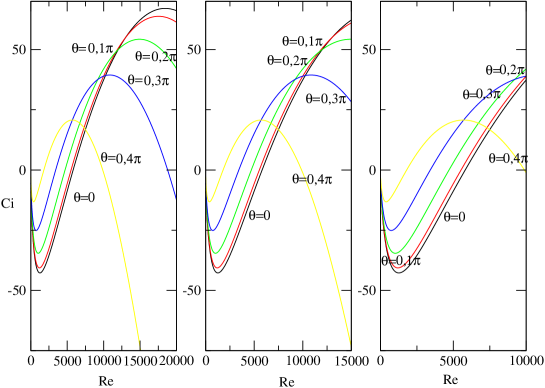
Figure 1: (a) Growth rate $C_{i}$ vs. Reynolds number $Re$ for $k=1$; (b) zoom of (a) to small values of k; (c) zoom of (b) to small values of $Re$.

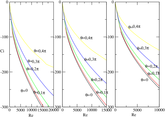
Figure 2: (a) Growth rate $C_{i}$ vs. Reynolds number $Re$ for $k=2$; (b) zoom of (a) to small values of k; (c) zoom of (b) to small values of $Re$.

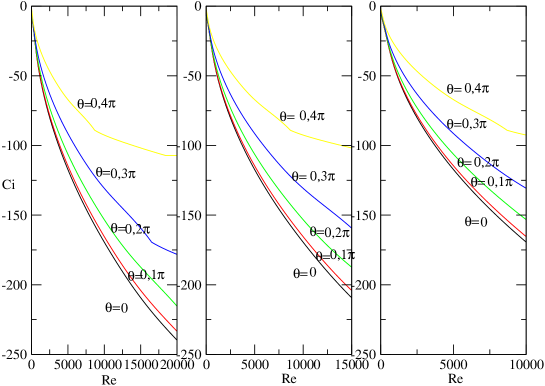
Figure 3: (a) Growth rate $C_{i}$ vs. Reynolds number $Re$ for $k=4$; (b) zoom of (a) to small values of k; (c) zoom of (b) to small values of $Re$.

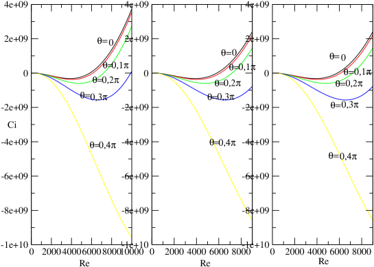
Figure 4: (a) Growth rate $C_{i}$ vs. Reynolds number $Re$ for $k=1$; (b) zoom of (a) to small values of k; (c) zoom of (b) to small values of $Re$.

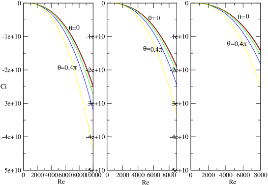
Figure 5: (a) Growth rate $C_{i}$ vs. Reynolds number $Re$ for $k=2$; (b) zoom of (a) to small values of k; (c) zoom of (b) to small values of $Re$.

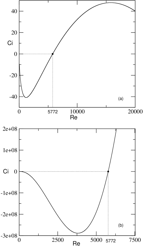
Figure 6: (a) Growth rate $C_{i}$ vs. Reynolds number $Re$ for $k=1.02$ in the case of inertial effects normalization showing the critical Reynolds number for $2D$-disturbances; (b) Growth rate $C_{i}$ vs. Reynolds number $Re$ for $k=1.02$ in the case of viscous effects normalization showing the critical Reynolds number for $2D$-disturbances.

6 Conclusion

In this paper, we have investigated the stability of boundary layer in Poiseuille flow. We have shown that the instability of the perturbed flow is governed by a remarkably equation named modified Orr-Sommerfeld equation. Contrary to what one might think, we find that Squire’s theorem is not applicable for the boundary layer. We find also that normalization by inertial or viscous effects leads to the same order of stability or instability. For the $2D$ disturbances flow ($\theta=0$), we found the same critical Reynolds number for our two normalizations. This value coincides with the one we know for neutral stability of the known Orr-Sommerfeld equation. We noticed also that for all overs values of $k$ in the case $\theta=0$ correspond the same values of $Re_{\delta}$ at $c_{i}=0$ whatever the normalization. We therefore conclude that in the boundary layer with a 2D-disturbance, we have the same neutral stability curve whatever the normalization.

References

- [1] J. G. Oldroyd. On the formulation of rheological equations of state. Proc. Roy. Soc. London Ser. A. 200 (1950), 523–541. MR 11,703a.
- [2] T. C. Ho and M. M. Denn. Stability of plane Poiseuille flow of a highly elastic liquid. J. Non- Newtonian Fluid Mech. 3 (1977), 179–195. Zbl 414.76008.
- [3] Bertolotti, F. P., Herbert, T. and Spalart.P. R Linear and nonlinear stability of the Blasius boundary layer.J. Fluid Mech, 1992, 242, 441–474.
- [4] K. C. Lee and B. A. Finlayson. Stability of plane Poiseuille and Couette flow of a Maxwell fluid. J. Non-Newtonain Fluid Mech. 21 (1986), 65–78. Zbl 587.76059.
- [5] R. C. Lock. The stability of the flow of an electrically conducting fluid between parallel planes under a transverse magnetic field. Proc. Roy. Soc. London Ser. A. 233 (1955), 105–125. MR 18,700a.
- [6] Abu-Ghannam, B. and Shaw, R. Natural transition of boundary layers - the effects of turbulence, pressure gradient, and flow history. J. Mech. Eng. Sci.1980- 22 (5), 213–228.
- [7] Andersson, P., Berggren, M. and Henningson, D. Optimal disturbances and bypass transition in boundary layers. Phys.Fluids 11 (1),1999, 134–150.
- [8] Andersson, P., Henningson, D. and Hanifi, A. On a stabilization procedure for the parabolic stability equations. J. Eng. Math.1998, 33, 311–332.
- [9] Landau, L. & Lifchitz, E. M. Fluid Mechanics. Butterworth Heinemann, Oxford, 1997.
- [10] Ray, Samad, and Chaudhury: Department of Mathematics, University of Burdwan, Burdwan-713104, West Bengal, India.