A new phase of scalar field with a kinetic term non-minimally coupled to gravity

Abstract

We consider the dynamics of a scalar field non-minimally coupled to gravity in the context of cosmology. It is demonstrated that there exists a new phase for the scalar field, in addition to the inflationary and dust-like (reheating period) phases. Analytic expressions for the scalar field and the Hubble parameter, which describe the new phase are given. The Hubble parameter indicates an accelerating expanding Universe. We explicitly show that the scalar field oscillates with time-dependent frequency. Moreover, an interaction between the scalar field in the new phase and other fields is discussed. It turns out that the parametric resonance is absent, which is another crucial difference between the dynamics of the scalar field in the new phase and dust-like phase.

I INTRODUCTION

To solve the flatness problem and the horizon problem in cosmology, Alan Guth introduced the inflation paradigm guth . The simple model, which is a single scalar field (inflaton) with minimally coupling to gravity, is described by an action

$$S=\int d^{4}x\sqrt{-g}\left[-\frac{R}{2\kappa^{2}}-\frac{1}{2}g^{\mu\nu}\partial_{\mu}\varphi\partial_{\nu}\varphi-V(\varphi)\right],$$ (1)

where $\displaystyle\kappa^{2}\equiv 8\pi G$. Although model (1) with quadratic potential, $\displaystyle V(\varphi)=\frac{1}{2}m^{2}\varphi^{2}$, is consistent with the cosmic microwave background CMB-data , many models have been proposed to produce the inflation era bassett . Regarding the motivations, many attempts are devoted to derive the inflation era by more fundamental principles or find connections between inflaton and other fields that are used in particle physics(e.g. Higgs field) bassett ; mukhanov ; Germani .
An intuitive picture of the dynamics of inflaton is as follows: the inflaton field rolls slowly down its potential (inflationary period), eventually the field(s)oscillates around the minimum of its potential and decays into light particles (reheating period). It has been assumed that the reheating period takes place just after the inflationary period. Also, since the inflaton has lost its energy, it behaves like dust matter in the reheating period.
For the quadratic potential, this intuitive picture is supported by analytic methods mukhanov , ( see quartic for the quartic potential). Usually model builders use the stated scenario for their models ( see ghalee for a different scenario). Then, they set limits on the parameters of the models. So, one can divide the dynamics of inflaton in two phases; inflationary phase and matter dominate phase(near minimum of the potential).
In this work, we show that in the following effective action

$$S=\int d^{4}x\sqrt{-g}\left[-\frac{R}{2\kappa^{2}}-\frac{1}{2}(g^{\mu\nu}-\alpha^{2}G^{\mu\nu})\partial_{\mu}\varphi\partial_{\nu}\varphi-V(\varphi)\right],$$ (2)

where $\displaystyle G^{\mu\nu}$ is Einstein’s tensor, the scalar field has a new phase. Germani et.al Germani , proposed the above action with quartic potential, $\displaystyle\lambda\varphi^{4}$, in the context of the new Higgs inflation. The cosmological perturbation of the model and reheating period of the model have been studied in Germani2 and mohseni respectively.
This paper is organized as follows: in §II we briefly review the model and obtain equations, then we qualitatively discuss why the scalar field of model (2), has a new phase for any typical potential,$\displaystyle V(\varphi)$. In §III analytic solutions for the Hubble parameter and the scalar field are provided for the quadratic potential. The solutions describe the new phase of the scalar field. In §IV we investigate an implication of the new phase by considering an interaction between a relativistic field and the scalar field. To introduce reader to the method that is used in this paper, we re-derive solution of the scalar field of the model (1) in reheating period in Appendix A, which is identical with the solution in the textbook mukhanov . Appendix B is devoted to some properties of the Fresnel integrals.

II Evidences for existence of the new phase

To obtain field equation and the Friedman equation of the model in FRW background metric, we use the ADM formalism with the following metric ansatz wald

$$ds^{2}=-N(t)dt^{2}+a(t)^{2}\delta_{ij}dx^{i}dx^{j}.$$ (3)

By inserting this expression into (2) we have Germani ; Germani2

$$S=\int dta^{3}\left[-3\frac{H^{2}}{\kappa^{2}N}+\frac{1}{2}\frac{\dot{\varphi}^{2}}{N}+\frac{3}{2}\frac{H^{2}\alpha^{2}\dot{\varphi}^{2}}{N^{3}}-NV(\varphi)\right],$$ (4)

by varying the action(4) with respect to the laps $\displaystyle N$ and $\displaystyle\varphi$ and setting $\displaystyle N$ to 1, we obtain

$$\begin{split}&H^{2}=\frac{\kappa^{2}}{6}\left[\dot{\varphi}^{2}(1+9\alpha^{2}H^{2})+2V(\varphi)\right],\cr&\ddot{\varphi}(1+3H^{2}\alpha^{2})+3H\dot{\varphi}(1+3H^{2}\alpha^{2})+6\dot{\varphi}H\dot{H}\alpha^{2}=-\frac{dV(\varphi)}{d\varphi}.\end{split}$$ (5)

The behavior of the scalar field can be divided into two regimes note1

• If $\displaystyle\alpha H\ll 1$, from (5) we have

  $$\displaystyle H^{2}=\frac{\kappa^{2}}{6}\left[\dot{\varphi}^{2}+2V(\varphi)\right],$$ (6a)

  $$\displaystyle\ddot{\varphi}+3H\dot{\varphi}=-\frac{dV(\varphi)}{d\varphi}.$$ (6b)

Equations (6a) and (6b) are the same as equations which are derived from (1) and studied in textbooks mukhanov ; Weinberg . Since we want to compare other regime with this regime, we quote the main results.
The second term on the left hand side of (6b), which is always positive, acts as a dissipative force. Therefore, the scalar filed rolls toward the minimum of the potential, and it behaves as a dust matter. For the simplest potential,$\displaystyle V(\varphi)=\frac{1}{2}m^{2}\varphi^{2}$, it has been shown that mukhanov

$$H(t)=\frac{2}{3t}\quad,\quad\varphi(t)=\frac{\sqrt{6}H(t)}{\kappa m}\cos\left[mt+g(0)\right]$$ (7)

where $\displaystyle g(0)$ is an arbitrarily constant. It is important to note that expressions in (7) are only valid for $\displaystyle H(t)<m$, so higher order terms, have been neglected mukhanov .

• If $\displaystyle\alpha H\gg 1$, from (5) we have

  $$\displaystyle H^{2}=\frac{\kappa^{2}}{6}\left[\dot{\varphi}^{2}9\alpha^{2}H^{2}+2V(\varphi)\right],$$ (8a)

  $$\displaystyle\ddot{\varphi}-3H\dot{\varphi}w_{eff}=-\frac{1}{3H^{2}\alpha^{2}}\frac{dV(\varphi)}{d\varphi},$$ (8b)

  where $\displaystyle w_{eff}$ is the effective equation of state

  $$w_{eff}=-1-\frac{2}{3}\frac{\dot{H}}{H^{2}}\quad.$$ (9)

The inflationary phase of this regime, $\displaystyle w_{eff}\rightarrow-1$, was studied in Germani ; Germani2 . Note that during the inflationary phase, the second term on the left hand side in (8b) is positive, and acts as a dissipative force. So, again, the scalar filed rolls toward the minimum of the potential , but at $\displaystyle H=2/3t$, it is vanished and, after some time, its sign may be changed and act as a driving force. Another point is that the right hand side of (8b), depends on $\displaystyle H$, which is not constant in this period. This behavior, shows that we need a different analysis for this regime.

III Explicit solutions for the quadratic potential

In this section we consider the simple potential $\displaystyle V(\varphi)=\frac{1}{2}m^{2}\varphi^{2}$, then we seek solutions for the equations. We use the so-called averaging method Guckenheimer , which is used in study of nonlinear differential equations. In Appendix A, we use this method to re-derive (7).
Let us define a new time variable $\displaystyle\tau$ as

$$t=\int\frac{3\alpha H}{m}d\tau,$$ (10)

It is worth to mention that this step is only a trick to solve the equations, when we obtain the solutions we’ll back to the original time variable, $\displaystyle t$.
Combining Eqs. (8a),(8b) and (10), with the quadratic potential, gives

$$\begin{split}&H^{2}=\frac{\kappa^{2}}{6}m^{2}\left(\varphi^{\prime 2}+\varphi^{2}\right),\cr&\varphi^{\prime\prime}+\left(\frac{H^{\prime}}{H}+\frac{9H^{2}\alpha}{m}\right)\varphi^{\prime}=-3\varphi,\end{split}$$ (11)

where prime denotes the differential with respect to $\displaystyle\tau$.
In order to use the method of averaging, we define the following relations Guckenheimer

$$\displaystyle\varphi=\frac{\sqrt{6}H}{\kappa m}\cos\left(\tau+f(\tau)\right),$$ (12a)

$$\displaystyle\varphi^{\prime}=\frac{-\sqrt{6}H}{\kappa m}\sin\left(\tau+f(\tau)\right),$$ (12b)

where $\displaystyle f(\tau)$ is an arbitrary function. Differentiation of the righthand side of (12a) must be equals to the righthand side of (12b). Hence we have

$$H^{\prime}\cos\left(\tau+f(\tau)\right)=Hf^{\prime}\sin\left(\tau+f(\tau)\right),$$ (13)

Substitution of (12a) and (12b) into (11) results in

$$\begin{split}&2H^{\prime}\sin\left(\tau+f(\tau)\right)+Hf^{\prime}\cos\left(\tau+f(\tau)\right)\cr&+\frac{9H^{3}\alpha}{m}\sin\left(\tau+f(\tau)\right)-2H\cos\left(\tau+f(\tau)\right)=0.\end{split}$$ (14)

$\displaystyle H^{\prime}$ and $\displaystyle f^{\prime}$ can be found from Equations (13) and (13) as

$$\begin{split}&f^{\prime}=\frac{\cos\left(\tau+f(\tau)\right)}{1+\sin^{2}\left(\tau+f(\tau)\right)}\left[2\cos\left(\tau+f(\tau)\right)-\frac{9H^{2}\alpha}{m}\sin\left(\tau+f(\tau)\right)\right]\cr\\ &H^{\prime}=\frac{H\sin\left(\tau+f(\tau)\right)}{1+\sin^{2}\left(\tau+f(\tau)\right)}\left[2\cos\left(\tau+f(\tau)\right)-\frac{9H^{2}\alpha}{m}\sin\left(\tau+f(\tau)\right)\right].\end{split}$$ (15)

So far we have not used any approximation for $\displaystyle H$, and $\displaystyle f(\tau)$. In the method of averaging, equations in (15) are replaced by averaged expressions. For this goal, note that if we keep $\displaystyle H$ and $\displaystyle f$ fixed noteref , the righthand side of (15) are $\displaystyle\pi$-periodic in $\displaystyle\tau$, so we can average over $\displaystyle\tau$.
By applying the stated procedure, one can show that

$$\begin{split}&\left<\frac{\cos^{2}\left(\tau+f(\tau)\right)}{1+\sin^{2}\left(\tau+f(\tau)\right)}\right>=\sqrt{2}-1,\left<\frac{\sin^{2}\left(\tau+f(\tau)\right)}{1+\sin^{2}\left(\tau+f(\tau)\right)}\right>=1-\frac{\sqrt{2}}{2},\cr&\left<\frac{\cos\left(\tau+f(\tau)\right)\sin\left(\tau+f(\tau)\right)}{1+\sin^{2}\left(\tau+f(\tau)\right)}\right>=0,\end{split}$$ (16)

where $\displaystyle<\cdots>\equiv\oint(\cdots)d\tau/\pi$ denotes an average over $\displaystyle\tau$ (but $\displaystyle H$ and $\displaystyle f$ are fixed). So, from Eqs. (15) and (16), we have

$$\begin{split}&f^{\prime}=2(\sqrt{2}-1)\cr&H^{\prime}=-\frac{9H^{3}\alpha}{m}(1-\frac{\sqrt{2}}{2}).\end{split}$$ (17)

The averaged equations are very easy to solve:

$$H(\tau)=\left[\frac{18\alpha}{m}(1-\frac{\sqrt{2}}{2})\tau\right]^{\frac{-1}{2}},\hskip 7.22743ptf(\tau)=2(\sqrt{2}-1)\tau.$$ (18)

We can use formula (10) and (18) to obtain explicit relation between $\displaystyle\tau$ and $\displaystyle t$ as

$$t=2\left[\frac{2m}{\alpha}(1-\frac{\sqrt{2}}{2})\right]^{\frac{-1}{2}}\tau^{\frac{1}{2}}.$$ (19)

By using Eqs. (18) and (19) we have

$$H(t)=\frac{2}{3(2-\sqrt{2})t}$$ (20)

so, the effective equation of state becomes

$$w_{eff}=-1-\frac{2}{3}\frac{\dot{H}}{H^{2}}\approx-0.41.$$ (21)

Moreover, from (12a) and (19), we also obtain

$$\varphi(t)=\frac{\sqrt{6}H(t)}{\kappa m}\cos\left[\frac{m}{2\alpha}(2-\sqrt{2})(\sqrt{2}-\frac{1}{2})t^{2}\right]$$ (22)

where $\displaystyle H(t)$ is given by (20).
The new phase of the scalar field is described by (20) and (22). According to (21), for this new phase we have $\displaystyle w_{eff}<-1/3$, so, the Universe is driven to accelerated expansion phase by the scalar field. Expression (22), shows that the scalar field oscillates with time-dependent ”frequency”, as indicated in Fig.1. Both of the properties are more different than the dust-like phase, which is described by (7).

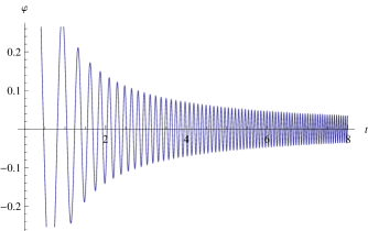
Figure 1: The scalar field versus $\displaystyle t$ for $\displaystyle\kappa m=10$, $\displaystyle m=10\alpha$ (with $\displaystyle\hbar=c=1$). Compare with Fig[1] in the first and the second papers of mohseni

IV An Implication

In this section, to show an implication of properties of the new phase, we will consider an interaction between a matter field,$\displaystyle\chi$, and the scalar field.
The decay of the scalar field into a relativistic field can be described by mukhanov

$$\mathcal{L}_{int}=-\frac{1}{2}g^{2}\varphi^{2}\chi^{2}.$$ (23)

It has been shown that if the interaction takes place during the dust-like phase, the parametric resonance instability is occurred parametric resonance ; mukhanov .
Notice that this result is obtained if the expansion of the universe is neglected. The stated assumption, seems to be a reasonable condition, at least for the first approximation, if the rate of interaction is too fast compared to the Hubble expansion time, see discussions about this note in mukhanov . As mentioned in mukhanov , what one actually finds from present of the parametric resonance, is that the perturbative analysis is rather misleading, during dust-like phase of the inflaton.
Here,our aim is to quest for the parametric resonance, during the new phase of the scalar field.
If the other scalar field, $\displaystyle\chi$, is decomposed into Fourier modes as

$$\chi(\vec{X},t)=\frac{1}{(2\pi)^{3/2}}\int d^{3}k\left(\chi^{*}_{k}(t)e^{i\vec{k}.\vec{X}}+\chi_{k}(t)e^{-i\vec{k}.\vec{X}}\right),$$ (24)

then using (22) and (23), the following equation for the Fourier modes is obtained

$$\ddot{\chi_{k}}+\left(k^{2}+g^{2}A^{2}\cos^{2}(M^{2}t^{2})\right)\chi_{k}=0,$$ (25)

where

$$A^{2}\equiv\frac{6}{\kappa^{2}}\frac{H^{2}}{m^{2}},\qquad M^{2}\equiv\frac{m}{2\alpha}(2-\sqrt{2})(\sqrt{2}-\frac{1}{2}).$$ (26)

Now, following mukhanov , we will neglect the expansion of space. So, If we define the following variables

$$\xi\equiv\sqrt{2}Mt,\quad\omega^{2}\equiv\frac{k^{2}+g^{2}A^{2}}{2M^{2}},\quad\varepsilon\equiv\frac{g^{2}A^{2}}{4M^{2}},$$ (27)

it thus follows that

$$\frac{d^{2}\chi_{k}}{d\xi^{2}}+(\omega^{2}+\varepsilon\cos\xi^{2})\chi_{k}=0.$$ (28)

To obtain an approximate solution for $\displaystyle\chi_{k}$, we expand $\displaystyle\chi_{k}$ as

$$\chi_{k}=\chi^{0}_{k}+\varepsilon\chi^{1}_{k}+\ldots\quad.$$ (29)

The expression (29) is valid, if $\displaystyle\chi^{1}_{k}$ has not terms that grow without bound as $\displaystyle t\rightarrow\infty$. So, it is necessary to cross-check this condition after we obtain an explicit expression for $\displaystyle\chi^{1}_{k}$.
Substituting (29) into (28), and keeping all terms up to second-order in $\displaystyle\varepsilon$, yields

$$\begin{split}&\frac{d^{2}\chi^{0}_{k}}{d\xi^{2}}+\omega^{2}\chi^{0}_{k}=0\\ &\frac{d^{2}\chi^{1}_{k}}{d\xi^{2}}+\omega^{2}\chi^{1}_{k}=-\chi^{0}_{k}\cos\xi^{2}.\end{split}$$ (30)

The first equation in (30) gives

$$\chi^{0}_{k}=b_{1}\sin\omega\xi+b_{2}\cos\omega\xi,$$ (31)

where $\displaystyle b_{1}$ and $\displaystyle b_{2}$ are the integration constants.
Using (31) and the following variables

$$u\equiv\sqrt{\frac{2}{\pi}}(\xi+\omega),\qquad v\equiv\sqrt{\frac{2}{\pi}}(\xi-\omega),$$ (32)

the second equation in (30) can be solved as

$$\begin{split}\chi^{1}_{k}=&Q_{1}\cos(\omega\xi)+Q_{2}\sin(\omega\xi)-\frac{1}{4\omega}\sqrt{\frac{\pi}{2}}\bigg{\{}\\ &\cos(\omega\xi+\omega^{2})[b_{{}_{1}}C(u)-b_{2}S(u)]+\\ &\sin(\omega\xi+\omega^{2})[b_{{}_{2}}C(u)+b_{1}S(u)]+\\ &\cos(\omega\xi-\omega^{2})[b_{{}_{1}}C(v)+b_{2}S(v)]+\\ &\sin(\omega\xi-\omega^{2})[b_{{}_{2}}C(v)-b_{1}S(v)]+\\ &2C(\frac{u+v}{2})[b_{2}\sin(\omega\xi)-b_{1}\cos(\omega\xi)]\bigg{\}}.\end{split}$$ (33)

Where $\displaystyle Q_{1}$, $\displaystyle Q_{2}$, are the integration constants, and $\displaystyle C(x)$, $\displaystyle S(x)$ are the Fresnel integrals ( see Appendix B).
From properties of the Fresnel integralsAbramowitz , we conclude that expression (33) has not any terms that grow without bound as $\displaystyle t\rightarrow\infty$. So, the parametric resonance is absent in (25). Therefore, we expect that the perturbation approximation for $\displaystyle\chi$, which is given by (29), is assured for all times.
Figure 2 compares the approximate solution for $\displaystyle\chi$, to the numerical solution. The two curves are almost indistinguishable.
If we used (25) instead of (6b), we would have terms that grow without bound as $\displaystyle t\rightarrow\infty$, which are sources of the parametric resonance during dust-like phase of the scalar field.

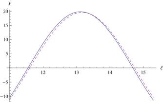
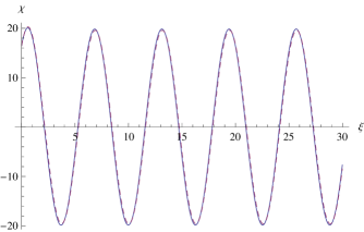
Figure 2: The relativistic field,$\displaystyle\chi$, versus $\displaystyle\xi$. Solid line represents the numerical solution. Dashed line represents the approximate solution. Where the parameters are chosen such that $\displaystyle\chi=16.5$, $\displaystyle\frac{d\chi}{d\xi}=12$. The two curves are so similar that it is almost impossible to distinguish between them, as shown in 2.

Appendix A

In this appendix, to show the power of the method that is used in this paper, we re-derive (7), by the averaging method.
By introducing $\displaystyle\beta\equiv mt$, and $\displaystyle V(\varphi)=\frac{1}{2}m^{2}\varphi^{2}$, equations (6a) and (6b) can be written to give

$$\begin{split}&H^{2}=\frac{m^{2}\kappa^{2}}{6}\left[\dot{\varphi}^{2}+\varphi^{2}\right],\cr&\ddot{\varphi}+3\frac{H}{m}\dot{\varphi}=-\varphi\ .\end{split}$$ (34)

Now, consider the following relations

$$\displaystyle\varphi=\frac{\sqrt{6}H}{\kappa m}\cos\left(\beta+g(\beta)\right),$$ (35a)

$$\displaystyle\varphi^{\prime}=\frac{-\sqrt{6}H}{\kappa m}\sin\left(\beta+g(\beta)\right),$$ (35b)

where $\displaystyle g(\beta)$ is an arbitrary function. Differentiation of the righthand side of (35a) must be equals to the righthand side of (35b). Hence we have

$$H^{\prime}\cos\left(\beta+g(\beta)\right)=Hg^{\prime}\sin\left(\beta+g(\beta)\right),$$ (36)

Substitution of (35a) and (35b) into (34) yield

$$\begin{split}&H^{\prime}\sin\left(\beta+g(\beta)\right)+Hg^{\prime}\cos\left(\beta+g(\beta)\right)\cr&+\frac{3H^{2}}{m}\sin\left(\beta+g(\beta)\right)=0.\end{split}$$ (37)

By algebraic manipulations, $\displaystyle H^{\prime}$ and $\displaystyle g^{\prime}$ can be found from Equations (36) and (37) as

$$\begin{split}&g^{\prime}=-\frac{3H}{2m}\sin\left(\beta+g(\beta)\right)\cos\left(\beta+g(\beta)\right)\cr\\ &H^{\prime}=-\frac{3H^{2}}{m}\sin^{2}\left(\beta+g(\beta)\right).\end{split}$$ (38)

These expression for $\displaystyle H$, and $\displaystyle g(\beta)$ are exact.
The advantage of the averaging method is that an approximation to the solution of (38) can be obtained by replacing (38) with its averaged equations as follows: if we keeping $\displaystyle H$ and $\displaystyle g$ fixed, the righthand side of (38) are $\displaystyle\pi$-periodic in $\displaystyle\beta$. By noting that

$$\left<\sin^{2}\left(\beta+g(\beta)\right)\right>=\frac{1}{2},\quad\left<\cos\left(\beta+g(\beta)\right)\sin\left(\beta+g(\beta)\right)\right>=0,$$ (39)

where $\displaystyle<>$ is used to indicate that we average over $\displaystyle\beta$, the averaged equations can be solved as

$$H(t)=\frac{2}{3t}\quad,\quad g(t)=g(0),$$ (40)

where g(0) is an arbitrary constant. Using (35a) and (40), we have

$$\varphi(t)=\frac{\sqrt{6}H(t)}{\kappa m}\cos\left[mt+g(0)\right]$$ (41)

where $\displaystyle H(t)$ is given by (40).
According to the averaging method, the above expressions for Hubble parameter and the scalar field are valid for $\displaystyle H(t)<m$. The results are the same as those obtained in mukhanov , which are also valid for $\displaystyle H(t)<m$.

Appendix B

The Fresnel integrals are defined by Abramowitz

$$\begin{split}&C(x)\equiv\int^{x}_{0}\cos(\frac{1}{2}\pi x^{2})dx\\ &S(x)\equiv\int^{x}_{0}\sin(\frac{1}{2}\pi x^{2})dx\end{split}$$ (42)

A series expansion for $\displaystyle x<1$ gives

$$\begin{split}&C(x)=\sum^{\infty}_{n=0}\frac{(-1)^{n}(\pi/2)^{2n}}{(2n)!(4n+1)}\hskip 2.84526ptx^{4n+1},\\ &S(x)=\sum^{\infty}_{n=0}\frac{(-1)^{n}(\pi/2)^{2n+1}}{(2n+1)!(4n+3)}x^{4n+3}.\end{split}$$ (43)

Therefore, $\displaystyle\lim_{x\rightarrow 0}C(x)=\lim_{x\rightarrow 0}S(x)=0$.
Asymptotic expansion of the integral are given by

$$\begin{split}&C(x)=\frac{1}{2}+\frac{1}{\pi x}\sin(\frac{1}{2}\pi x^{2}),\\ &S(x)=\frac{1}{2}-\frac{1}{\pi x}\cos(\frac{1}{2}\pi x^{2}).\end{split}$$ (44)

Hence, $\displaystyle\lim_{x\rightarrow\infty}C(x)=\lim_{x\rightarrow\infty}S(x)=1/2$.

References

- (1) A. H. Guth Phys. Rev. D23, 347 (1981).
- (2) E. Komatsu et al. [ WMAP Collaboration ], [arXiv:1001.4538 [astro-ph.CO]].
- (3) B. A. Bassett, S. Tsujikawa and D. Wands, Rev. Mod. Phys. 78, 537 (2006).
- (4) E. Komatsu et al. [ WMAP Collaboration ], [arXiv:1001.4538 [astro-ph.CO]].
- (5) V. Mukhanov, ”Physical Foundations of Cosmology,”Cambrdige Uni. Press (2005).
- (6) C. Germani, A. Kehagias, Phys. Rev. Lett.105, 011302 (2010).
- (7) S. Weinberg, “Cosmology,”Oxford, UK: Oxford Univ. Pr. (2008).
- (8) P. B. Greene, L. Kofman, A. Linde, A. A. Starobinsky Phys. Rev. D 56, 6175,(1997).
- (9) A. Maleknejad, M. M. Sheikh-Jabbari, Phys.Rev.D 84 043515,(2011); A. Ghalee, Phys.Lett.B 717, 307, (2012)
- (10) C. Germani, A. Kehagias JCAP 84, 043515 (2010).
- (11) H. Mohseni Sadjadi, P. Goodarzi JCAP 02 038 (2013); H. Mohseni Sadjadi, P. Goodarzi, [arXiv:1302.1177[gr- qc]].
- (12) R. M. Wald, General Relativity, Chicago, Usa: Univ. Pr. ( 1984)
- (13) It is worth noting that, in this work, we focus on solving the equations and study some physical consequences of the solutions. For this purpose, the constrains on the parameters of the model, e.g , which was obtained in Germani2 , are not important for us. So, our classification of the regimes, is not in chronological order. As we will see, this classification is suitable to discuss the difference between(1) and (2).If one like to stick to the constrains on parameters, which are obtained in Ref. Germani ; Germani2 ; mohseni ,we have the new phase, (7), and then dust-like phase, (22).
- (14) J. Guckenheimer and P. Holmes, Nonlinear Oscillations, Dynamical Sys-tems, and Bifurcations of Vector Fields , Springer-Verlag, (1981).
- (15) Physicaly, it means that we integrate out ”fast” modes, so, in fact, and are slowly varying functions. For further information about this subject see Guckenheimer .
- (16) L. Kofman, A. D. Linde, A. A. Starobinsky, Phys. Rev. Lett 73, 3195 (1994); R. Allahverdi, R. Brandenberger, F. Cyr-Racine and A. azumdar Annu. Rev. Nucl. Part. Sci. 60 27 (2010).
- (17) M. Abramowitz, I. A. Stegun “Handbook of Mathematical Functions,”New York: Dover Publications. (1965).