The dynamic conductivity of strongly non-ideal plasmas: is the Drude model valid?

Abstract

The method of moments is used to calculate the dynamic conductivity of strongly coupled fully ionized hydrogen plasmas. The electron density $n_{e}$ and temperature $T$ vary in the domains $10^{21}<n_{e}<10^{24}{\rm cm}^{-3}$, $10^{4}{\rm K}<T<10^{6}{\rm K}$. The results are compared to some theoretical data.

PACS: 51.10.+y, 51.70.+f, 52.25.Fi, 52.27.Gr, 52.80.Pi

1 Introduction

The determination of the (internal) dynamic conductivity (i.e., the response to the homogeneous high-frequency Maxwellian electrical field $\vec{E}(t)=\vec{E_{0}}{\rm exp}(-i\omega t))$ of dense plasmas has been a subject of substantial investigation for a long time. One of the reasons is that on the basis of this quantity all other plasma dynamic characteristics can be found [1]. There are two basic approaches to these studies: the generalized Drude-Lorentz model, see [2], the review [3] and references therein, and the method of moments [4]. Additionally, we have been working on the direct extension of the modified random-phase approximation for the calculation of the static conductivity $\sigma_{0}$, [5].

Previously, in [6], we applied the latter approach in the range of slightly and moderately non-ideal plasmas with the number density of electrons $n_{e}$ and temperature varying within the following limits: $10^{17}<n_{e}<10^{19}{\rm cm}^{-3}$, $10^{3}{\rm K}<T<10^{4}{\rm K}$ and examined the range of frequencies that covered the microwave and far-infrared region. In [5, 7] we extended the range of frequencies up to the ultraviolet radiation and covered the area of very high values of the electron density: $10^{21}<n_{e}<10^{23}{\rm cm}^{-3}$ with $10^{3}{\rm K}<T<10^{5}{\rm K}$.

The classical Drude-Lorentz formula for the plasma optical conductivity,

$$\sigma_{DL}(\omega)=\frac{\sigma_{0}}{1-i\omega\tau},\qquad\tau=\frac{4\pi\sigma_{0}}{\omega_{p}^{2}},$$ (1)

where $\sigma_{0}$ is static conductivity, and $\omega_{p}=\sqrt{4\pi n_{e}e^{2}/m}$ being the plasma frequency, predicts a monotonic decrease of its real part when the frequency $\omega\rightarrow\infty$, and it is not clear whether this property is maintained in real dense plasmas.

In the present work we study the question of monotonicity of the real part of the dynamic conductivity in even wider ranges of variation of the plasma parameters.

2 The model

We consider the (internal) dynamic conductivity of hydrogen plasmas in a volume $V$ containing $N_{e}=n_{e}V$ electrons and the same number of ions.

As a starting point for the computations we use the exact relation for the optical conductivity of Coulomb systems stemming from the theory of moments [8]

$$\sigma(\omega)=\frac{i\omega_{p}^{2}}{4\pi}\frac{\omega+q(\omega)}{\omega^{2}-\Omega^{2}+\omega q(\omega)},$$ (2)

where $q(\omega)$ is the boundary value of some analytic (Nevanlinna) function $q(z)$, which admits the representation

$$q(z)=ih+2z\int_{0}^{\infty}\frac{du(\omega)}{\omega^{2}-z^{2}},$$ (3)

with $h\geq 0$ and a non-decreasing bounded function $u(\omega)$ such that

$$\int\limits_{-\infty}^{\infty}\frac{du(\omega)}{1+\omega^{2}}<\infty.$$

Independently of the choice of $q\left(z\right)$, the optical given by the expression (2), has the following exact asymptotic expansion [8]

$$\sigma(\omega\rightarrow\infty)\simeq\frac{i\omega_{p}^{2}}{4\pi\omega}+\frac{i\omega_{p}^{2}\Omega^{2}}{4\pi\omega^{3}}+o(\frac{1}{\omega^{3}}).$$ (4)

The estimates for the characteristic frequency $\Omega$ [8] are provided in the next section. The parameter function $q(z)$ possesses no phenomenological meaning, but we can observe that the condition $\lim\limits_{\omega\rightarrow 0}q(\omega)=ih=4\pi i\sigma_{0}\left(\Omega/\omega_{p}\right)^{2}$ is equivalent to the definition $\lim\limits_{\omega\rightarrow 0}\sigma(\omega)=\sigma_{0}$. Hence, the simplest formula providing an interpolation between the exact asymptotic expansion (4) and the static conductivity has the following form:

$$\sigma(\omega)=\frac{i\omega_{p}^{2}}{4\pi}\frac{\omega+i\tau\Omega^{2}}{\omega^{2}-\Omega^{2}+i\omega\tau\Omega^{2}}.$$ (5)

We have previously calculated the plasma static conductivity in a wide range of plasma thermodynamic parameters, see [6, 5]. We used this data and also carried out additional computations of $\sigma_{0}$ using the same self-consistent field method [9] (for recent results obtained using this approach see [10]) to find the values of the transport relaxation time $\tau$ in an extended realm of the $n_{e}-T$ plane. Certainly, to evaluate the static conductivity one can employ alternative theoretical approaches like that of [11].

Notice that (5) turns into the classical Drude-Lorentz formula when $\Omega^{2}\rightarrow\infty$, i.e, when the asymptotic expansion (4) reduces to that satisfied by the Drude-Lorentz dynamic conductivity, $\sigma_{DL}(\omega\rightarrow\infty)\simeq i\omega_{p}^{2}/4\pi\omega+o(\omega^{-1}).$

3 The parameter $\Omega^{2}$

To estimate the dimensionless parameter

$$H=\Omega^{2}/\omega_{p}^{2}=h_{ei}\left(0\right)/3=\left(2\pi^{2}n_{e}\right)^{-1}\int_{0}^{\infty}k^{2}S_{ei}\left(k\right)dk,$$

at least in strongly coupled hydrogen plasmas, one can use the interpolation procedure suggested in [8]: approximate the static electron-ion structure factor $S_{ei}\left(k\right)$ at a zero Matsubara frequency [12]

$$S_{ei}\left(k\right)=P_{e}\left(k\right)P_{i}\left(k\right)/\left[k^{2}\lambda^{2}+P_{e}\left(k\right)+P_{i}\left(k\right)\right],$$ (6)

but, to go beyond the RPA, put the ion and electron dimensionless polarization operators (simple loops) as

$$P_{i}\left(k\right)=\Pi_{i}(k)/n_{e}\beta=1,\quad P_{e}\left(k\right)=\Pi_{e}(k)/n_{e}\beta=\gamma^{4}\lambda^{2}/\left(k^{2}+\gamma^{4}\lambda^{2}\right);$$ (7)

this interpolation being constructed to satisfy both the long- and short-wavelength limiting conditions [13, 8]:

$$P_{e}\left(k=0\right)=1,\quad P_{e}\left(k\longrightarrow\infty\right)\simeq\gamma^{4}\lambda^{2}/k^{2}$$ (8)

with

$$\gamma^{4}=16\pi n_{e}e^{2}m/\hbar^{2},\quad\lambda^{-2}=4\pi e^{2}n_{e}\beta.$$ (9)

Then by simple integration one gets [14]:

$$H=\left(4r_{s}/3\right)\sqrt{\Gamma/\left(3\Gamma^{2}+4r_{s}+4\Gamma\sqrt{6r_{s}}\right)}.$$ (10)

Observe that in weakly coupled plasmas with $\Gamma\longrightarrow 0$,

$$H\simeq\left(2/3\right)\sqrt{r_{s}\Gamma}\sim\sqrt{\beta}.$$ (11)

Table 1: The dimensionless static conductivity $\sigma_{0}/\omega_{p}$ as a function of electron density and temperature.

$n_{e}\cdot 10^{-22}({\rm cm}^{-3})$	$T=2\cdot 10^{4}{\rm K}$	$T=3\cdot 10^{4}{\rm K}$	$T=5\cdot 10^{4}{\rm K}$
$1$	$0.23$	$0.26$	$0.32$
$10$	$0.36$	$0.38$	$0.41$
$100$	$0.78$	$0.80$	$0.81$

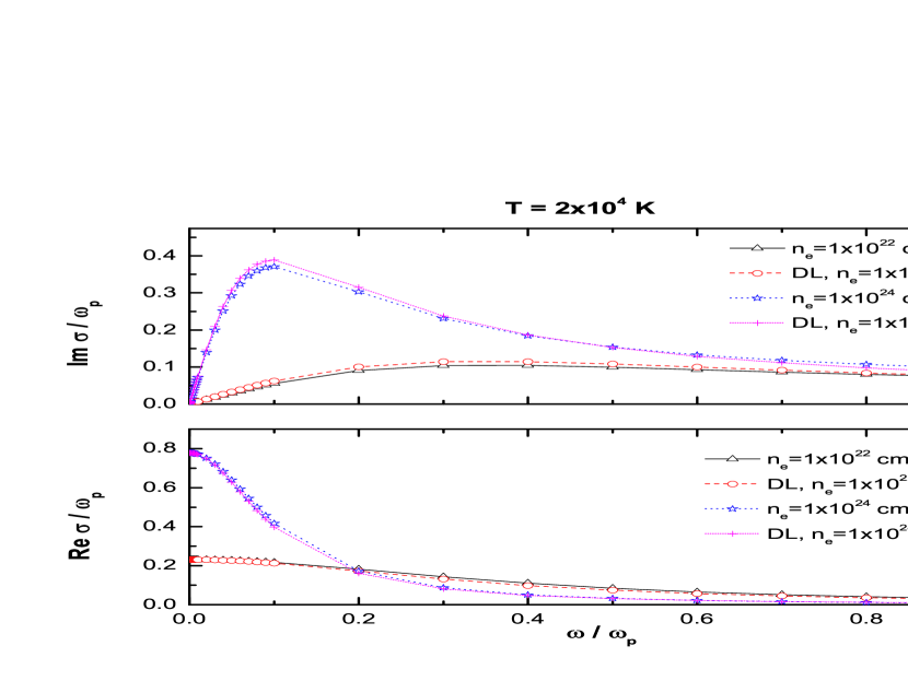
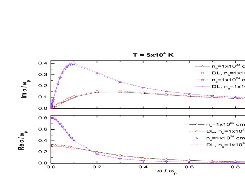
Figure 1: Dynamic conductivity of dense plasmas according to (5) compared to the Drude model (1) prediction. The static conductivity is provided in table 1.

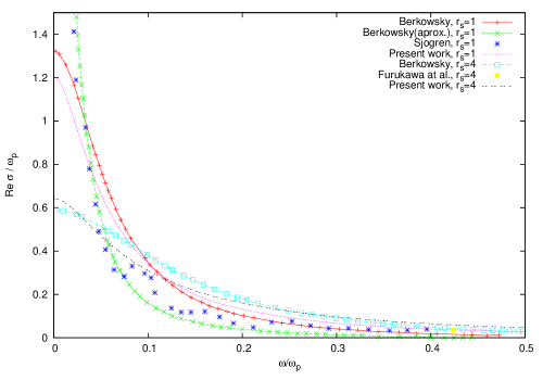
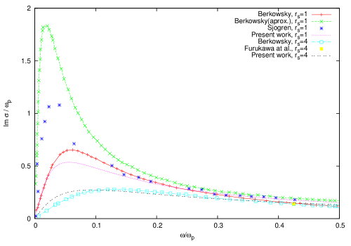
Figure 2: Data calculated from (5) for $\Gamma=0.5,r_{s}=1$ and $r_{s}=4$, as a function of ($\omega/\omega_{p}$) frequency ratio, together with results of other authors [15].

4 Results and discussion

The calculations of the real and imaginary parts of $\sigma(\omega)$ in (5) were carried out in the domain $10^{21}\leq n_{e}\leq 10^{24}{\rm cm}^{-3}$ and $10^{4}{\rm K}\leq T\leq 10^{6}{\rm K}$.

In the figure 1 we compare some of these results to those corresponding to the Drude-Lorentz model (1). For the reference we provide also the data for the dimensionless static conductivity $\sigma_{0}/\omega_{p}$, see table 1.

We observe that within the present model no qualitative difference exists between our results and those of the Drude-Lorentz model (1). Quantitative difference decreases as $\Gamma\rightarrow 0.$ It is evident that whenever $\xi=\left(1-\tau^{2}\Omega^{2}/2\right)>0$, the real part of (5) acquires an additional maxima at $\omega_{m}=\pm\Omega\sqrt{\xi}$, but for our data the values of $\xi$ are always negative.

Additionally, we successfully compare the data on $\sigma(\omega;n_{e},T)$ determined in this paper to the data from [15] for $\Gamma=0.5$, $r_{s}=1$ and $r_{s}=4$. The corresponding curves are shown in Fig. 2.

Detailed comparison of our results to those of other approaches, in particular, those described in [3], is due. We conclude that our results can be used for the investigation of dynamic and static properties of strongly coupled plasmas.

5 Acknowledgments

The presented work is performed within the Project 141033 financed by the Ministry of Science of Republic Serbia and is supported by the Spanish Ministerio de Ciencia e Innovación (Project No. ENE2007-67406-C02-02/FTN) and the INTAS (GSI-INTAS Project 06-1000012-8707).

6 References

References

- [1] Kobzev G A, Iakubov I T, Popović M M (eds)1995 Transport and Optical Properties of Nonideal Plasma (New York:Plenum) chapter 6.2
-
[2]
Reinholz H, Redmer R, Röpke G, Wierling A 2000 Phys. Rev.
E 62 5648-666;
Reinholz H, Morozov I, Röpke G, Millat Th 2004 Phys. Rev. E 69 066412 - [3] Reinholz H 2005 Ann. Phys. Fr. 30 1-187
- [4] Adamyan V M, Tkachenko I M 2003 Lectures on physics of non-ideal plasmas, part I, Odessa State University, Odessa, 1988, in Russian; Contrib. Plasma Phys. 43 252-7
- [5] Adamyan V M, Djurić Z, Mihajlov A A, Sakan N M, Tkachenko I M 2004 J. Phys. D 37 1896-903
- [6] Mihajlov A A, Djurić Z, Adamyan V M, Sakan N M 2001 J. Phys. D 34 3139-144
- [7] Adamyan V M, Grubor D, Mihajlov A A, Sakan N M, Srećković V A, Tkachenko I M 2006 J. Phys. A 39 4401-405
- [8] Adamyan V M, Tkachenko I M 1983 High Temp. 21 307-14
-
[9]
Adamyan V M, Guly G A, Pushek N L, Starchik P D,
Tkachenko I M, Shvets I S 1980 High Temp. 18 186-93;
Tkachenko I M, Fernández de Córdoba P 1998 Phys. Rev. E 57 2222-9 - [10] Alcober J and Tkachenko I M 2008 Int. Conf. Strongly Coupled Coulomb Systems (SCCS2008), Book of Abstracts (Camerino, Italy, July-August, 2008) p 90
-
[11]
Redmer R 2000 High Pressure Research 16 345-57;
Kuhlbrodt S, Redmer R 2000 Phys. Rev. E 62 7191-200;
Esser A, Redmer R, Röpke G 2003 Contrib. Plasma Phys. 43 33-8;
Kuhlbrodt S, Holst B, Redmer R 2005 Contr. Plasma Physics 45 73-88 - [12] Abrikosov A A, Gorkov L P, Dzyaloshinski I E 1965, Methods of Quantum Field Theory in Statistical Physics (Oxford:Pergamon)
- [13] Bonch-Bruevich V L, Tiablikov S V 1962 The Green function method in statistical mechanics (New York: Interscience) .
- [14] Corbatón M J and Tkachenko I M 2008 Int. Conf. Strongly Coupled Coulomb Systems (SCCS2008), Book of Abstracts (Camerino, Italy, July-August 2008) p 90
- [15] Berkovsky M A, Djordjević D, Kurilenkov Yu K, Milchberg H M, Popović M M 1991 J. Phys. B 24 5043-53