Black Hole Formation with an Interacting Vacuum Energy Density: Curvature Effects

Abstract

The gravitational collapse of a spherically symmetric massive core of a star in which the fluid component is interacting with a growing vacuum energy density filling a FLRW type geometry with an arbitrary curvature parameter is investigated. The complete set of exact solutions for all values of the free parameters are obtained and the influence of the curvature term on the collapsing time, black hole mass and other physical quantities are also discussed in detail. We show that for the same initial conditions the total black hole mass depends only on the effective matter density parameter (including the vacuum component). It is also shown that the analytical condition to form a black hole i.e. the apparent horizon is not altered by the contribution of the curvature terms, however, the remaining physical quantities are quantitatively modified.

I Introduction

In the current view of cosmology, the present accelerating stage of the Universe is caused by the dark energy component, usually represented by a cosmological constant $\Lambda$ Riess ; Komatsu . Its contribution to the Einstein Field Equations (EFE) is the same of a perfect simple fluid with constant equation of state (EoS) parameter $\omega\equiv p/\rho=-1$, being interpreted as the net energy density stored on the vacuum state of all quantum fields pervading the observed Universe rev1 .

Although in agreement with the existing astronomical observations (both at background and perturbative levels), $\Lambda$ is plagued with the longstanding cosmological constant problem, i.e. the huge discrepancy ($\sim$ 120 orders of magnitude) between the theoretical expectations ($\rho_{v}\sim 10^{106}eV^{4}$) from quantum field theory by assuming that the natural cutoff is related to gravity (Planck’s energy) and the present day ($\rho_{v}\sim 10^{-16}eV^{4}$) cosmological bounds Zeldovich67 ; zee85 ; Weinberg . The simplest manner to alleviate such a problem is to introduce some dynamics, or equivalently, to replace its constant value, say, $\Lambda_{0}$, by a time dependent quantity, $\Lambda(t)\equiv 8\pi G\rho_{v}(t)$, where $\rho_{v}$ is the vacuum energy density (from now on a subscript zero denotes the present day value of a quantity). In this way, the incredible small value of $\Lambda$ is the result of a continuous decaying vacuum process i.e. the value of $\Lambda$ is small nowadays because the Universe is too old.

Many sources for a dynamical vacuum energy density have been proposed in the literature sources , and several phenomenological models based on different decay laws for $\Lambda(t)$ were also discussed even before the discovery of the acceleration of the Universe OT86 ; L1 ; CLW ; L2 ; L3 . Decay $\Lambda(t)$ models were the predecessors of all interacting dark energy models being until nowadays a very active field of the current research L5 ; new1 ; ML02 ; EA1 ; Harko11 ; LBS2012 .

As happens with the cosmic history, a dynamical $\Lambda(t)$-term can also affect the formation of black holes. However, for each evolving system, the interacting vacuum behaves in a quite different manner. In the expanding Universe, for instance, the vacuum energy density is a continuously time dependent decreasing function while for black hole formation $\rho_{v}(t)$ is a growing quantity in the course of the collapsing process. In the later case, one may ask whether the increasing repulsive gravitational force (due to the negative vacuum pressure) may prevent the ultimate formation of a singularity.

Recently, Campos and Lima CL12 (henceforth paper I) discussed the formation of black holes (and naked singularities) during the gravitational collapse of a fluid interacting with a time-varying vacuum in the context of a flat Friedmann-Lemaitre-Robertson-Walker (FLRW) geometry. For given initial conditions, they solved analytically the basic equations describing the evolution of the two-fluid interacting mixture and analyzed the development of the apparent horizons before the formation of the singularity. It was shown that a time-varying vacuum energy density increases the collapsing time but, in general, it cannot prevent the formation of black holes. Their results also suggested that the cosmic censorship hypothesis (CCH), at least in its weak form, can generically violated in the presence of a time varying vacuum due to the formation of naked singularities. In this concern, many authors have discussed how naked singularities can observationally be distinguished from black holes through strong gravitational lensing effects and the physics of accretion disks naked .

In this paper, we go one step further by analyzing the influence of the curvature on the results derived in Paper I. As we shall see, following a unified method first proposed by Assad and Lima AL88 for a one component expanding simple fluid, we obtain the complete set of collapsing exact solutions for all values of the free parameters describing the interacting mixture. The influence of the curvature on the collapsing time, black hole mass and other physical quantities are also discussed in detail. In particular, it is found that for the same initial conditions the black hole mass depends only on the effective matter density parameter and that naked singularities are also formed for a large interval of the physical parameters. It is also shown that the analytical condition to form a black hole i.e. the apparent horizon is not altered by the contribution of the curvature terms, however, the remaining physical properties are quantitatively modified.

II Collapsing star with variable - $\Lambda(t)$

II.1 Geometry and Composition of the Collapsing Star Medium

To begin with, we first remark that the basic discussion here is related to black holes and naked singularities formed from collapsing star cores. In this way, the formation process involving supermassive black holes like the ones found in the galactic centers will not be investigated here.

Let us now consider that the massive core of a star medium is formed by a mixture of a isotropic simple fluid plus a growing vacuum energy density. Inside the core it will be assumed that the spacetime is described by a generic FLRW geometry ($c=1$):

$$ds^{2}_{-}=dt^{2}-a^{2}\left(t\right)\left(\frac{dr^{2}}{{1-k\,r^{2}}}+r^{2}d\Omega^{2}\right),$$ (2.1)

where $a\left(t\right)$ is the scale factor, $k=0,\pm 1$ is the curvature parameter and $d\Omega^{2}\equiv d\theta^{2}+\sin^{2}\theta d\varphi^{2}$ is the area element on the unit sphere. Such an approximation must work at least for the late stages of the collapsing process. The complete spacetime may be divided into 3 different regions, namely: $V^{\pm}$ and $\Sigma$, where $V^{+}$($V^{-}\;$) is the exterior (interior) of the massive core, and $\Sigma$ denotes the surface of the massive collapsing core. Following standard lines, in this paper we shall focus our attention mainly in the spacetime inside the star core CaiWang ; CL12 .

The EFE inside the star medium can be written as:

$$G_{-}^{\mu\nu}=8\pi G\left[{T_{-}^{\mu\nu}}_{(f)}+{T_{-}^{\mu\nu}}_{(v)}\right],$$ (2.2)

where $G_{-}^{\mu\nu}$ is the Einstein tensor and ${T_{-}^{\mu\nu}}_{(f)}$, ${T_{-}^{\mu\nu}}_{(v)}$ are the energy-momentum tensor (EMT) of the fluid component and vacuum, respectively. ${T_{-}^{\mu\nu}}_{(v)}\equiv\rho_{v}g_{-}^{\mu\nu}$, where $\rho_{v}=\Lambda(t)/8\pi G$.

The Einstein tensor is divergenceless, and, therefore, the EFE imply that a variable-$\Lambda(t)$ is possible if at least one of the two following conditions are satisfied: (i) ${T_{-}^{\mu\nu}}_{(f)}$ is not separately conserved, i.e., ${T_{-}^{\mu\nu}}_{(f)};_{\nu}\neq 0$, and (ii) ${T_{-}^{\mu\nu}}_{(f)};_{\nu}=0$ but $G$ is a time dependent quantity VariableG . In this paper we assume that the fluid and vacuum components are interacting and G is constant.

    

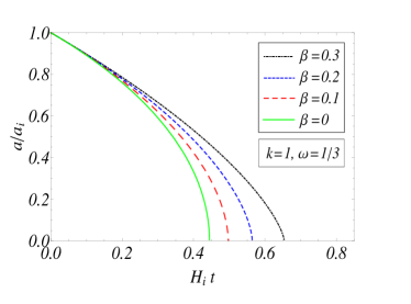
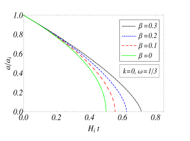
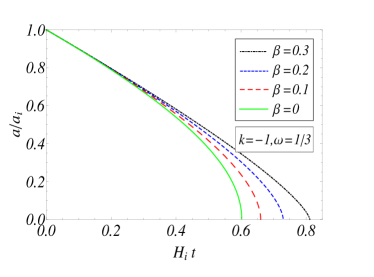
Figure 1: Evolution of the scale factor for closed, flat and hyperbolic geometries. The star fluid is represented by a vacuum component interacting with radiation ($\omega=1/3$). The overall effect of the vacuum component for any geometry is to increase the collapsing time relatively to a pure fluid medium ($\beta=0$). Note also that for a selected value of $\beta$, the collapse process in closed models ($k=+1$) is favored as compared to the flat case. In the hyperbolic geometry ($k=-1$) we have the opposite effect.

II.2 Basic Equations and Solutions

In the background given by Eq. (2.1), the EFE for the interacting mixture (perfect fluid plus a vacuum component) can be written as:

$$8\pi G\rho_{f}+\Lambda\left(t\right) = 3H^{2}+\frac{3k}{a^{2}},$$ (2.3)

$$8\pi Gp_{f}-\Lambda\left(t\right) = -2\dot{H}-3H^{2}-\frac{k}{a^{2}},$$ (2.4)

where a dot means time derivative, $H=\dot{a}/a<0$ is the “Hubble function” and $\rho_{f}$, $p_{f}$ are, respectively, the energy density and pressure of the fluid component which obeys the equation of state

$$p_{f}=\omega\rho_{f}\,,$$ (2.5)

where $0\leq\omega\leq 1$ is a constant parameter. The energy conservation law which is is contained in the EFE equations reads:

$$\dot{\rho}_{f}+3\frac{\dot{a}}{a}\left(\rho_{f}+p_{f}\right)\ =-\dot{\rho}_{v}.$$ (2.6)

For the sake of generality, in what follows we consider that the $\Lambda(t)$-term is given by:

$$\Lambda=\Lambda_{0}+3\beta H^{2}+3\beta\frac{k}{a^{2}},$$ (2.7)

where $\beta$ is a dimensionless constant parameter and the factor 3 was added for mathematical convenience CLW . This form is a natural extension of the $\Lambda$-term used in the Paper I (see Eq.(9) there) including the curvature effect. As one may check, it means that the fraction

$$\beta=\frac{\rho_{v}-\rho_{vo}}{\rho_{f}+\rho_{v}},$$ (2.8)

remains constant during the collapsing process. Such an expression generalizes the expression derived by Solá and Shapiro SS within a renormalization group approach ($k=0$) and also the one proposed by Carvalho et al. CLW by including a bare cosmological constant $\Lambda_{0}$.

Now, by using expressions (2.5) and (2.7), it is easy to check that the differential equation governing the scale factor takes the form:

$$a\ddot{a}+\Delta\,\dot{a}^{2}+\Delta k-\Lambda_{0}(1+\omega)a^{2}/2=0,$$ (2.9)

where $\Delta=-1+3(1+\omega)(1-\beta)/2$. By integrating the above equation we obtain for the first integral:

$$\dot{a}^{2}=b\left(\frac{a_{i}}{a}\right)^{2\Delta}-k+\frac{\Lambda_{0}a^{2}}{3(1-\beta)},$$ (2.10)

where $b=(a_{i}H_{i})^{2}+k-\frac{\Lambda_{0}a_{i}^{2}}{3(1-\beta)}$ is a constant, and $a_{i}$, $H_{i}$ are the initial values for the scale factor and the Hubble parameter.

Since $\Lambda_{0}$ is very small, once the collapse process has initiated under the pull of the core self gravitation ($a<<a_{i}$) the term containing $\Lambda_{0}$ can be surely neglected. Hence, in what follows we will retain only the curvature term in order to quantify its effect on the black hole mass and other physical quantities. In this case, the full integration of the field equations can be performed by introducing the auxiliary variable

$$u=\frac{k}{b}\left(\frac{a}{a_{i}}\right)^{2\Delta},$$ (2.11)

which transforms Eq.(2.10) to

$$\dot{u}=\frac{2b^{1/2}\left({k}/{b}\right)^{A}}{\left(2A-1\right)a_{i}\,}u^{1-A}\,\sqrt{1-u}\,,$$ (2.12)

where $A=\frac{1+\Delta}{2\Delta}$.

The inversion of Eq.(2.12) results

$$\frac{dt}{du}=\frac{\left(2A-1\right)a_{i}\,b^{A-\frac{1}{2}}}{2k^{A}}\frac{u^{A-1}}{\sqrt{1-u}}\,,$$ (2.13)

and combining with the second derivative we find

$$u(1-u)\frac{d^{2}t}{du^{2}}+\left[(1-A)-\left(\frac{3}{2}-A\right)u\right]\frac{dt}{du}=0\,.$$ (2.14)

The above Eq. (2.14) is a particular case of the hypergeometric differential equation with parameters $\alpha_{1}=0$, $\alpha_{2}=\frac{1}{2}-A$, and $\alpha_{3}=1-A$, and whose solution is given by Abra

$$t(u)=c_{1}+c_{2}u^{A}F\left(\frac{1}{2},A;1+A;u\right),$$ (2.15)

where $c_{1}$ and $c_{2}$ are arbitrary constants and $F(\alpha_{1},\alpha_{2},\alpha_{3},u)$ is the hypergeometric Gaussian function Abra . Considering the initial condition $a(t=0)=a_{i}$, and that for $t=t_{c}\rightarrow a=0$, we can write the above solution as

$$\left(1-\frac{t}{t_{c}}\right)=\left(\frac{a}{a_{i}}\right)^{1+\Delta}\frac{F\left(\frac{1}{2},A;1+A;\cfrac{k}{b}\,\left(\cfrac{a}{a_{i}}\right)^{2\Delta}\right)}{F\left(\frac{1}{2},A;1+A;\cfrac{k}{b}\right)}\,,$$ (2.16)

where

$$t_{c}=\frac{H_{i}^{-1}F(1/2,A;1+A;\frac{k}{b})}{(1+\Delta)\sqrt{1+k/a_{i}^{2}H_{i}^{2}}}\,,$$ (2.17)

is the total collapsing time. As one may check, since $F(\alpha_{1},\alpha_{2},\alpha_{3},0)=1$, where $\alpha_{i}$ are arbitrary parameters of the hypergeometric function, we see that for $k\rightarrow 0$ the above expressions assume the simpler forms

$$\frac{a}{a_{i}} = \left(1-\frac{t}{t_{c}}\right)^{\frac{2}{3(1+\omega)(1-\beta)}}\,,$$ (2.18)

$$t_{c} = \frac{2H_{i}^{-1}}{3(1+\omega)(1-\beta)}\,,$$

which are identical to the solutions previously obtained by Campos and Lima for the flat case (see Eqs. (12) and (13) of Paper I).

It is worth noticing that for all values of $\beta$ and k, the modulus of the initial Hubble function ($H_{i}$) sets the collapsing time scale to reach the singular point ($a(t_{c})=0$), (see Eq. (2.17)). However, for $\beta=1$ the collapsing time $t_{c}\rightarrow\infty$ and, in this case, the spacetime is nonsingular (pure de Sitter vacuum). As in the Paper I, henceforth it will be assumed that the vacuum parameter is restricted on the interval $0\leq\beta<1$.

         

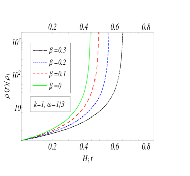
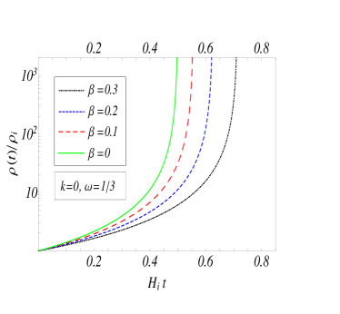
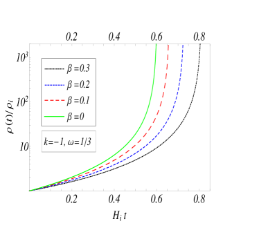
Figure 2: Evolution of the total energy density for closed, flat and open geometries. For all cases the two fluid mixture is formed by a vacuum component interacting with a radiation fluid ($\omega=1/3$). Note that the evolution of the energy densities depend on the values of the $\beta$ and curvature parameters.

In Figure 1 we show the evolution of the scale factor as a function of the dimensionless time $H_{i}t$. Different values for $\beta$ were selected for three distinct cases: (i) a radiation filled core ($\omega=1/3$) coupled to a vacuum growing component and a positive curvature; (ii) an identical scenario to the anterior case with null curvature; (iii) finally, we consider a negative curvature parameter. Notice that for a fixed curvature parameter, the collapsing time increases for higher values of $\beta$. However, for a given value of $\beta$, models with positive (negative) curvature present a smaller (higher) collapsing time relatively to the flat case. For the sake of completeness, we close this section on exact results by exhibiting the expressions for the vacuum and fluid energy densities:

$$\rho_{v} = \rho_{vi}\left(\frac{a_{i}}{a}\right)^{3(1+\omega)(1-\beta)}\,,$$ (2.19)

$$\rho_{f} = \rho_{fi}\left(\frac{a_{i}}{a}\right)^{3(1+\omega)(1-\beta)}\,,$$ (2.20)

where the initial densities, $\rho_{vi}$, $\rho_{fi}$, are related by the expression $\rho_{vi}=\frac{\beta}{1-\beta}\rho_{fi}$.

In Figure 2, we show the time behavior of the total energy density as a function of the dimensionless time parameter $H_{i}t$ and some selected values of the pair of free parameters ($\beta$, k). For all values of $\beta<1$, we see that the energy density diverges at the collapse time ($t_{c}$) which is strongly correlated with the values of $\beta$. As should also be expected (see Fig. 1) for a given value of $\beta$, the collapsing time is reduced (increased) for positive (negative) curvatures as compared to the flat scenario. In a more realistic treatment, a continuous transition from radiation ($\omega=1/3$) to to the Zeldovich’s stiff-matter fluid ($\omega=1$) may also occur at the late stages. Naturally, such a final state is included in the general solutions for $a(t)$ and $\rho(t)$ with similar plots appearing in Figs. 1 and 2.

II.3 Unified conformal time solutions

Some gain in simplicity is obtained by using the conformal transformation, $dt=a(\eta)d\eta$. In this case, the metric given by Eq.(2.1) becomes

$$ds^{2}=a(\eta)^{2}\left(d\eta^{2}-\frac{dr^{2}}{{1-k\,r^{2}}}-r^{2}d\Omega^{2}\right)\,,$$ (2.21)

while the motion equation (2.9) is transformed to:

$$aa^{\prime\prime}+(\Delta-1)a^{\prime 2}+k\Delta a^{2}=0\,.$$ (2.22)

Where the prime denotes conformal time derivative. Now, by introducing the auxiliary transformation $z=a^{\Delta}$, Eq.(2.9) takes the following forms (see AL88 ; Lima01 in the case $\beta=0$):

$$z^{\prime\prime}+k\Delta^{2}z=0\,.$$ (2.23)

This is a remarkable result for the interacting mixture. We see that the auxiliary scale factor obeys the same differential equation of a particle subject to a linear force regardless the values of $\beta$ and $\omega$. In particular, the flat case behaves like a free particle while for a closed geometry ($k=1$) we have an harmonic oscillator with angular “frequency” $f=|-1+3(1+\omega)(1-\beta)/2|$.

A simple integration of above equation yields:

$$a(\eta)=\left[c_{1}\sin\left(\eta\Delta\sqrt{k}\right)+c_{2}\cos\left(\eta\Delta\sqrt{k}\right)\right]^{1/\Delta}\,,$$ (2.24)

where $c_{1}$ and $c_{2}$ are arbitrary constants with the proviso that the first integral given by Eq.(2.10) must be obeyed, and we have used the inverse transformation $a=z^{\frac{1}{\Delta}}$.

With suitable initial conditions for the collapse process, the above solution can be rewritten as:

$$a(\eta)=a_{i}\left\{\sqrt{\frac{b}{k}}\sin{\sqrt{k}\Delta(\eta_{c}-\eta)}\right\}^{\frac{1}{\Delta}}\,,$$ (2.25)

where

$$\eta_{c}=\frac{1}{\Delta\sqrt{k}}\sin^{-1}\left[\sqrt{\frac{k}{b}}\right]\,,$$ (2.26)

is the collapsing time in the conformal coordinate. Inserting expression (2.25) into Eq.(2.16) we obtain the general solution for the collapsing time, $t(\eta)$, regardless of the equation of state and curvature parameters.

The hypergeometric function can be reduced to an elementary expression for specific values of the free parameters. In this case, the conformal solutions are readily obtained from the general expressions of a($\eta$) and t($\eta$). In order to exemplify that, let us now exhibit the explicit solutions describing the last stages of the collapsing core by assuming the Zeldovich stiff matter fluid ($\omega=1$) plus a vacuum component ($\beta=1/2$) for all values of the curvature parameter.

         

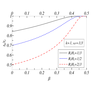
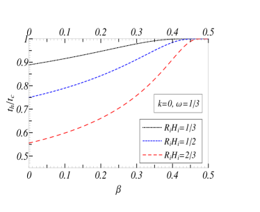
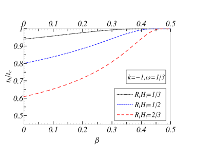
Figure 3: Ratio between the the time to develop the apparent horizon ($t_{AH}$) and collapsing time ($t_{c}$). The plots show the case of a radiation fluid for closed, flat and hyperbolic geometries. We see that the formation of the horizon is delayed for higher values of $\beta$. Note that the for a given value of $\beta$ the formation of the apparent horizon (as compared to the collapsing time) is slightly favored for closed models ($k=1$), and the inverse happens in the hyperbolic case ($k=-1$). We also remark that for $\beta>0.5$ the apparent horizon is not formed before the total collapsing time, and, therefore, the singularity is naked.

Let us first determine the unified form of the solutions. For $\omega=1$ and $\beta=1/2$ it follows that $\Delta=1/2$. In this case, from Eqs. (2.16) and (2.25), it is easy to see that the unified solution (for any curvature) can be written as:

$$a(\eta) = a_{i}\,b\left\{\sqrt{\frac{1}{k}}\sin\left[\sqrt{k}\,\frac{\eta_{c}-\eta}{2}\right]\right\}^{2},$$ (2.27)

$$t_{c}-t = \frac{a_{i}\,b}{2\,k}\left\{\eta_{c}-\eta-\frac{\sin\left[\sqrt{k}(\eta_{c}-\eta)\right]}{\sqrt{k}}\right\},\,$$ (2.28)

where $\eta_{c}$ is given by (2.26) with $\Delta=1/2$. Note also that the parameter $b=a_{i}^{2}H_{i}^{2}+k$ is still free to be fixed. By choosing $b=1$ we see that $H_{i}^{2}=(1-k)/a_{i}^{2}$. Therefore, for $k=1$ we have $H_{i}=0$ and the collapse process may start from the rest. In the simplified forms below we have fixed $b=1$ for all cases.

(i) Closed Solution:

$$a(\eta) = \frac{a_{i}}{2}(1+\cos\eta)\,,$$

$$t_{c}-t = \frac{a_{i}}{2}(\pi-\eta-\sin\eta)\,,$$

where the collapsing time is $t_{c}=a_{i}\eta_{c}/2$ and $\eta_{c}=\pi$, according to (2.17) and (2.26).

(ii) Hyperbolic Solution:

$$a(\eta) = \frac{a_{i}}{2}\left[\cosh(\eta_{c}-\eta)-1\right]\,,$$ (2.29)

$$t_{c}-t = \frac{a_{i}}{2}\left[\sinh(\eta_{c}-\eta)-(\eta_{c}-\eta)\right]\,,$$ (2.30)

where $\eta_{c}=2\ln(1+\sqrt{2})$, and $t_{c}=a_{i}(\sqrt{2}-\eta_{c}/2)$ is given by (2.17) and (2.26).

(iii) Flat solution:

$$1-\frac{t}{t_{c}} = \left(\frac{\eta_{c}-\eta}{2}\right)^{3}\,,$$ (2.31)

$$a(\eta) = a_{i}\left(\frac{\eta_{c}-\eta}{2}\right)^{2}\,,$$ (2.32)

where $\eta_{c}=2$, $t_{c}=2a_{i}/3$, and $a_{i}=H_{i}^{-1}$. Combining the above expressions one obtains the simplified form:

$$1-\frac{t}{t_{c}}=\left(\frac{a}{a_{i}}\right)^{3/2}\,,$$

as obtained before through a different method (see Eqs. (2.18)).

III Black hole formation and apparent horizons

An important issue on black hole physics is related to the formation of an apparent horizon during the collapsing process. In the present context such a subject deserves a closer scrutiny since the collapsing mixture involves a growing vacuum component.

On the other hand, by the cosmic censorship hypothesis, singular points must be dressed by apparent horizons i.e. naked singularities are forbidden RP69 . This means that when the system is approaching the singularity, an apparent horizon should be developed inside it (before the collapsing time $t_{c}$).

Nevertheless, such a conjecture is not true in general Papa and some examples have already been discussed in the literature Collapse . In the present case, the increasing negative pressure of the vacuum component can be responsible by the formation of a naked singularity. As we shall see next, for a given interval of the $\beta$ parameter, naked singularities can generically be formed for arbitrary values of the curvature.

The natural observers describing the behavior of the matter fields in the FLRW geometry are comoving with the fluid volume elements. Let us now define a constant geometrical radius ($r_{\Sigma}$) for the surface dividing the star interior from the exterior, For such surface, the metric can be written as:

$$ds^{2}_{\Sigma}=d\tau^{2}-R\left(\tau\right)^{2}d\Omega^{2}\,,$$ (2.33)

where $t=\tau$ and $R(t)=r_{\Sigma}a(\tau)$. Apparent horizons are defined by space-like surfaces with future point converging null geodesics on both sides of the surface Hawking ; Anninos . Naturally, for an initially untrapped star, the black hole is formed only when the apparent horizon appears before the singularity otherwise a naked singularity it will be the final stage of the collapsing core.

As discussed by many authors McV ; CM73 ; CaiWang , the formation of the apparent horizon is determined by the condition:

$$R_{,\alpha}R_{,\beta}g^{\alpha\beta}=\left(r_{\Sigma}\dot{a}\right)^{2}-1+kr_{\Sigma}^{2}=0\,,$$ (2.34)

where $()_{,x}=\frac{\partial}{\partial x}$ and $R(t,r)=a(t)r$.

Since the star is initially not trapped the comoving surface is spacelike. This means that

$$R_{,\alpha}R_{,\beta}g^{\alpha\beta}=\left[r\dot{a}\left(t_{i}\right)\right]^{2}-1+kr^{2}<0\,,$$ (2.35)

which implies that $0<(R_{i}H_{i})^{2}<1-kr^{2}$.

Another important quantity is the mass function that furnish the total mass inside the surface with radius $r$ at time $t$. Cahill and McVittie CM73 wrote such a function for a particular reference system that here takes the following form (see also Poisson )

$$m(t,r)=\frac{1}{2}R\left(1+R_{,\alpha}R_{,\beta}g^{\alpha\beta}\right)=\frac{1}{2}R(\dot{R}^{2}+kr^{2}).$$ (2.36)

As it appears, the first integral given by equation (2.10) can be rewritten in the variable $R=a(t)r$ by taking into account the constraint to form the apparent horizon

$$\dot{R}_{AH}^{2}+kr^{2}=b\,r^{2}\left(\frac{R_{i}}{R_{AH}}\right)^{2\Delta}=1\,,$$ (2.37)

and solving for the radius of the apparent horizon we obtain

$$\frac{R_{AH}}{R_{i}}=\left(R_{i}^{2}H_{i}^{2}+kr^{2}\right)^{\frac{1}{2\Delta}}\,.$$ (2.38)

On the other hand, at $t=t_{AH}$, the time evolution equation (2.16) implies that

$$\frac{t_{AH}}{t_{c}}=1-\left(\frac{R_{AH}}{R_{i}}\right)^{1+\Delta}\frac{F(1/2,A;1+A;\frac{k}{b}(\frac{R_{AH}}{R_{i}})^{2\Delta})}{F(1/2,A;1+A;\frac{k}{b})}.$$ (2.39)

Notice that for $k=0$ the above expression reduce to

$$t_{AH}/t_{c}=1-(R_{i}\,H_{i})^{\frac{1+\Delta}{\Delta}}\,,$$ (2.40)

which is exactly the same one previously obtained in Paper I with a slightly different notation (see Eq. (26) there).

In Figure 3, we show the behavior of the dimensionless ratio $t_{AH}/t_{c}$ as a function of $\beta$ parameter for a collapsing radiation fluid ($\omega=1/3$) in different geometries ($k=0,\pm 1$). For a selected value of $R_{i}H_{i}$, we see that the curvature effects are small in comparison to the flat case. Note also that in the examples displayed the formation of the apparent horizon happens before the emergence of the singularity.

     

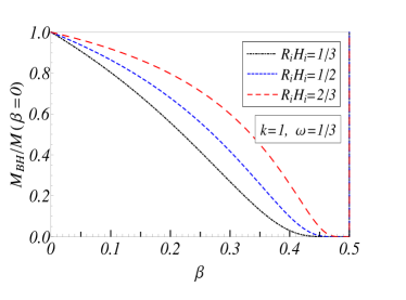
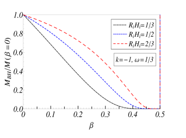
Figure 4: Black hole masses for closed, flat and hyperbolic geometries. The ratio between the mass of the BH formed and the mass of a pure fluid versus the $\beta$ parameter. For a fixed value of the product $H_{i}R_{i}$, we see that the BH mass is not only heavily dependent on the $\beta$ parameter but decreases for higher values of $\beta$. For $k=+1,0,-1$ the mass of the black hole formed diminishes, respectively. For all geometries we have adopted the Cahill and McVittie mass definition CM73 .

Following the same steps of paper I and using the mass definition given by Eq. (2.36) we can calculate the total mass of the black hole:

$$M(\tau_{AH})=M_{0}\left\{\frac{R_{i}^{2}H_{i}^{2}+kr^{2}}{(R_{i}H_{i})^{4\Delta}}\right\}^{\frac{1}{2\Delta}}\,,$$ (2.41)

where $M_{0}={R_{i}^{3}H_{i}^{2}}/{2}$ is the black hole mass for $k=\omega=0$. For a flat geometry ($k=0$) the above expression reduces to

$$M(\tau_{AH})=\frac{1}{2}R_{i}^{3}H_{i}^{2}(R_{i}H_{i})^{\frac{3(1+\omega)(1-\beta)-3}{1-\frac{3}{2}(1+\omega)(1-\beta)}}\,,$$ (2.42)

which is identical to the expression previously obtained in Paper I (cf. Eq.(29) there).

In terms of solar mass units such an expression can be rewritten as:

$$M(\tau_{AH})=R_{i}\frac{M_{\odot}}{r_{S\odot}}\left\{R_{i}H_{i}\sqrt{\Omega_{fi}/(1-\beta)}\right\}^{\frac{1}{\Delta}}\,,$$ (2.43)

where $M_{\odot}$ and $r_{S\odot}$ are respectively, the solar mass and the Schwarzschild radius of the sun. In the case of a fluid with $k=0$ one finds $\Omega_{fi}=1-\beta$ with the above expression reducing to

$$M(\tau_{AH})=\frac{R_{i}M_{\odot}}{r_{S\odot}}(R_{i}H_{i})^{\frac{2}{{{3}(1+\omega)(1-\beta)}-2}}.$$ (2.44)

Now, assuming $R_{i}=80\,Km$ and $R_{i}H_{i}\sim 1/2$ one finds $M\sim 13.3\,M_{\odot}$ for a pure radiation fluid ($\beta=0,\omega=1/3$). However, for $\beta=0.25$ and the same values of $R_{i}$ and $H_{i}$, one obtains a smaller mass, namely, $M\sim 6.6\,M_{\odot}$. Such results reproduce the values obtained in the paper I where $R_{i}$ was wrongly typed.

What about the influence of the curvature on the black hole mass? Taking into account identical conditions with a non null curvature is not difficult to conclude that the influence of the curvature is to mildly increase (decreases) the black hole mass for closed ($k=1$) and hyperbolic geometries, respectively. Since the black hole mass is a positive quantity, we can also infer from (2.43) that the vacuum parameter must satisfy

$$\beta\leq 1-\frac{2}{3(1+w)},$$ (2.45)

in order to form a black hole. For $\omega=1/3$ this inequality implies that $\beta\leq 0.5$ in agreement with the results presented in Figs. 3 and 4. Naturally, for $\beta>0.5$ the singularity of the fluid mixture (radiation plus vacuum) is naked.

IV Final Comments

In this paper we have discussed the collapsing process of a massive star core whose matter content is formed by a mixture of two interacting components: a simple fluid described by the EoS, $p=\omega\rho$, $\omega$=constant, and a growing vacuum component. Through an unified treatment we have taken into account the curvature effects. The vacuum energy density was supposed to satisfy the constraint $\rho_{v}=\beta\rho_{total}$ where $\beta$ is a constant. From the FLRW equations this means that the dynamical $\Lambda(t)$-term satisfies the relation CLW ; SS : $\Lambda(H,a)$ = $3\beta H^{2}+3\beta k/{a^{2}}$, where $k=0,\pm 1$. The fluid component satisfies all the energy conditions (weak, dominant and strong), but the vacuum component ($p_{v}=-\rho_{v}$) violates the strong energy condition (SEC).

The main results derived here can be summarized in the following statements:

(i) For all values of the curvature, the vacuum component though violating the SEC does not avoid the ultimate collapse of the massive core, i.e. the system reach the singular point for a broad range of the free parameters ($\omega$, $\beta$).

(ii) For a fixed value of the initial conditions and free parameters, we shown that the collapsing process is slightly favored for closed geometry relatively to the flat case. For negative curvature we have found the opposite effect.

(iii) The time to form the apparent horizon ($t_{AH}$) and the total collapsing time ($t_{c}$) were analytically obtained through a unique expression valid for all physical values of the free parameters $\omega$, $\beta$ and k (see Eq.(2.41)). More interesting, by using the ratio $t_{AH}/t_{c}$ was also possible to determine when black holes or naked singularities are formed.

(iv) The nature of the singularity is heavily dependent on the values of the $\beta$ parameter. For $\beta<1-2/3(1+\omega)$ a black hole is formed, however, if $\beta>1-2/3(1+\omega)$ an apparent horizon does not appear before the collapsing time $t_{c}$, and, therefore, the cosmic censorship conjecture is violated and a naked singularity is formed. The critical case, $\beta=1-2/3(1+\omega)$, defines the boundary between naked singularities and black holes. We stress that such a condition does not depend on the curvature. Th existence of naked singularities is related to the vacuum pressure, and, generically, it appears when negative pressures large enough take place in the mixture.

Finally, we emphasize that the main caveat of the model discussed here is related to the hypothesis of homogeneity and isotropy of the spacetime generated by the collapsing massive star core. Presumably, it must be approximately valid at the late stages of the collapse. Note also that the avoidance of the singularity was not possible even in the presence of the vacuum energy density, but, clearly, such a prediction can be only an artifact of the decaying model assumed in the present paper. The generality of such a result will be discussed in a forthcoming communication.

V Acknowledgments

This paper is dedicated to the late Professor Mario José Delgado Assad (UFPB-Brazil). His earlier contribution to the unified approach for FRW type cosmologies motivated the present work. The authors E.L.D.P. and M.C. are partially supported by a grant from CNPq and J.A.S.L. is partially supported by CNPq and FAPESP (No. 04/13668-0).

References

- (1) A. Riess et al., Astron. J. 116, 1009 (1998); S. Perlmutter et al., Nature, 391, 51 (1998); M. Kowalski et al., Astrophys. J. 686, 749 (2008); R. Amanullah et al., Astrophys. J. 716, 712 (2010).
- (2) D. N. Spergel et al., Astrophys. J. Suppl. 148, 175 (2003); D. N. Spergel et al. Astrophys. J. Suppl. Ser. 170, 377 (2007); E. Komatsu et al. Astrophys. J. 192, 18 (2011).
- (3) P. J. E. Peebles and B. Ratra, Rev. Mod. Phys. 75 559 (2003); T. Padmanabhan, Phys. Rept. 380, 235 (2003); J. A. S. Lima, Braz. Journ. Phys. 34, 194 (2004), astro-ph/0402109; E. J. M. Copeland and S. Tsujikawa, Int. J. Mod. Phys. D15, 1753 (2006); J. A. Frieman, M. S. Turner and D. Huterer, Ann. Rev. Astron. & Astrophys, 46, 385 (2008); M. Li et al., arXiv:1103.5870 (2011).
- (4) Ya. B. Zeldovich, Usp. Fiz. Nauk 94, 209 (1968) [Sov. Phys. Usp. 11, 381 (1968).
- (5) A. Zee, in High Energy Physics, Proceedings of the 20th Annual Orbis Scientiae, edited by B. Kursunoglu, S. L. Mintz, and A. Perlmutter (Plenum, New York, 1985).
- (6) S. Weinberg, Rev. Mod. Phys. 61, 1 (1989).
- (7) B. Ratra and P. J. E. Peebles, Phys. Rev. D 37, 3406 (1988); C. Wetterich, Astron. and Astrophys. 301, 321 (1995); P. G. Ferreira and M. Joyce, Phys. Rev. D 58, 023503 (1998); N. J. Poplawski, [arXiv:gr-qc/0608031v2] (2006).
- (8) M. Ozer and M. O. Taha, Phys. Lett. B 171, 363 (1986); Nucl. Phys. B 287 776 (1987).
- (9) K. Freese et al., Nucl. Phys. B 287, 797 (1987); W. Chen and Y-S. Wu, Phys. Rev. D 41, 695 (1990); D. Pavón, Phys. Rev. D 43, 375 (1991).
- (10) J. C. Carvalho, J. A. S. Lima, and I. Waga, Phys. Rev. D 46, 2404 (1992).
- (11) J. A. S. Lima and J. M. F. Maia, Phys. Rev. D 49, 5597 (1994); J. A. S. Lima and M. Trodden, Phys. Rev. D 53, 4280 (1996), astro-ph/9508049.
- (12) I. Waga, Astrophys. J. 414, 436 (1993); L. F. Bloomfield Torres and I. Waga, Mon. Not. R. Astron. Soc. 279, 712 (1996); A. I. Arbab and A. M. M. Abdel-Rahman, Phys. Rev. D 50, 7725 (1994); J. M. Overduin and F. I. Cooperstock, Phys. Rev. D 58, 043506 (1998);
- (13) R. G. Vishwakarma, Class. Quant. Grav. 17, 3833 (2000); M. V. John and K. B. Joseph, Phys. Rev. D 61, 087304 (2000); O. Bertolami and P. J. Martins, Phys. Rev. D 61, 064007 (2000); R. G. Vishwakarma, Class. Quant. Grav. 18, 1159 (2001); A. S. Al-Rawaf, Mod. Phys. Lett. A 16, 633 (2001).
- (14) M. K. Mak, J. A. Belinchon, and T. Harko, Int. J. Mod. Phys. D 14, 1265 (2002); M. R. Mbonye, Int. J. Mod. Phys. A 18, 811 (2003); J. V. Cunha and R. C. Santos, Int. J. Mod. Phys. D 13, 1321 (2004), astro-ph/0402169; J. S. Alcaniz and J. A. S. Lima, Phys. Rev. D 72, 063516 (2005), astro-ph/0507372; S. Carneiro and J. A. S. Lima, Int. J. Mod. Phys. A 20, 2465 (2005), gr-qc/0405141; R. Opher and A. Pelinson, Mon. Not. R. Ast. Soc. 362, 167 (2005); S. Carneiro, C. Pigozzo and H. A. Borges, Phys. Rev. D 74, 023532 (2006).
- (15) J. M. F. Maia and J. A. S. Lima, Phys. Rev. D 65, 083513 (2002), arXiv:astro-ph/0112091.
- (16) F. E. M. Costa, J. S. Alcaniz and J. M. F. Maia, Phys. Rev. D 77, 083516 (2008).
- (17) S. Basilakos, M. Plionis and J. A. S. Lima, Phys. Rev. D 82, 083517 (2010), arXiv:1006.3418; S. Basilakos, M. Plionis and J. Solà, Phys. Rev. D 82 083512 (2010), arXiv:1005.5592; T. Harko, F. S. N. Lobo, Shin’ichi Nojiri and Sergei D. Odintsov, Phys. Rev. D 84, 024020 (2011).
- (18) F. E. M. Costa, J. A. S. Lima and F. A. Oliveira, arXiv:1204.1864v1 [astro-ph.CO]; J. S. Alcaniz, H. A. Borges, S. Carneiro, J. C. Fabris, C. Pigozzo and W. Zimdahl, Phys. Lett. B 716, 165 (2012), arXiv:1201.5919; Pradhan, R. Jaiswal and R. K. Khare, Astrophys Space Sci. 343, 489 (2013); J. A. S. Lima, S. Basilakos and J. Solà, Mon. Not. R. Ast. Soc. (2013), In press, arXiv:1209.2802 [gr-qc];
- (19) M. Campos and J. A. S. Lima, Phy. Rev. D 86, 043012 (2012), arXiv:1207.5150 [gr-qc].
- (20) K. S. Virbhadra and G. F. R. Ellis, Phys. Rev. D 65, 103004 (2002); Z. Kovács and T. Harko, Phys. Rev. D 82, 124047 (2010); S. Sahu. M. Patil, D. Narashima and P. S. Joshi, Phys. Rev. D 86, 063010 (2012).
- (21) M. J. D. Assad and J. A. S. Lima, Gen. Rel. Grav. 20, 527 (1988). For a more detailed version see preprint from Brazilian Center of Research Physics, Brazil - CBPF/NF/050/86 (1986).
- (22) R-G. Cai and A. Wang, Phys. Rev. D 73, 063005 (2006).
- (23) O. Bertolami, Nuovo Cimento, 93 B, 36 (1986); J. C. Carvalho and J. A. S. Lima, Gen. Rel. Grav. 26 909 (1994); J. Solà and H. Stefancic, Mod. Phys. Lett. A 21, 479 (2006), arXiv:astro-ph/0507110.
- (24) I. L. Shapiro and J. Solà, JHEP 02, 006 (2002), hep-th/0012227; J. Phys. A 41, 164066 (2008). For a recent review see J. Solà, J. Phys. Conf. Ser. 283, 012033 (2011), arXiv:1102.1815.
- (25) M. Abramowitz and I. A. Stegun, Handbook of Mathematical Functions (Dover Publications, New York, 1964).
- (26) J. A. S. Lima, Am. J. Phys. 69, 1245 (2001), astro-ph/0109215.
- (27) R. Penrose, Nuovo Cimento Soc. Ital. Fis. 1 , 252, (1969).
- (28) A. Papapetrou, A Random Walk in Relativity and Cosmology, edited by N. Dadhich, J. K. Rao, J.V. Narlikar, and C. V. Vishveshwara (John Wiley & Sons, New York, 1985), p. 184.
- (29) P. S. Joshi, Global Aspects in Gravitation and Cosmology, Clarendon, Oxford, (1993); D. Christodoulou, Ann. Math. 140, 607 (1994). For more recent reviews, see, e.g., R. Penrose, in Black Holes and Relativistic Stars, edited by R. M. Wald (University of Chicago Press, 1998); A. Krolak, Prog. Theor. Phys. Suppl. 136, 45 (1999); P. S. Joshi, Pramana 55, 529 (2000), and P.S. Joshi, “Cosmic Censorship: A Current Perspective,” gr-qc/0206087 (2002); Gravitational Collapse End States, gr-qc/0412082 (2004), and references therein. A. Beesham, Pramana 77, 429 (2011).
- (30) S. W. Hawking and G. F. R. Ellis, The Large Scale Structure of Spacetime, Cambridge University Press, Cambridge (1973).
- (31) P. Anninos et al. Phys. Rev. D 50 3801 (1994).
- (32) M. E. Cahill and G. C. McVittie, J. Math. Phys. 11, 1382 (1970).
- (33) G. C. McVittie, Mon. Not. R. Astron. Soc. 93, 325 (1933).
- (34) E. Poisson and W. Israel, Phys. Rev. D 41 1796 (1990); A. Wang, J. F. Villas da Rocha, and N. O. Santos, Phys. Rev. D 56, 7692 (1997); J. F. Villas da Rocha, A. Wang, and N. O. Santos, Phys. Lett. A 255, 213 (1999); S. A. Hayward, Phys. Rev. D 70, 104027 (2004); Phys. Rev. Lett. 93, 251101 (2004).