Structure formation in inhomogeneous Early Dark Energy models

Abstract

We study the impact of Early Dark Energy fluctuations in the linear and non-linear regimes of structure formation. In these models the energy density of dark energy is non-negligible at high redshifts and the fluctuations in the dark energy component can have the same order of magnitude of dark matter fluctuations. Since two basic approximations usually taken in the standard scenario of quintessence models, that both dark energy density during the matter dominated period and dark energy fluctuations on small scales are negligible, are not valid in such models, we first study approximate analytical solutions for dark matter and dark energy perturbations in the linear regime. This study is helpful to find consistent initial conditions for the system of equations and to analytically understand the effects of Early Dark Energy and its fluctuations, which are also verified numerically. In the linear regime we compute the matter growth and variation of the gravitational potential associated with the Integrated Sachs-Wolf effect, showing that these observables present important modifications due to Early Dark Energy fluctuations, though making them more similar to $\Lambda$CDM model. We also make use of the Spherical Collapse model to study the influence of Early Dark Energy fluctuations in the nonlinear regime of structure formation, especially on $\delta_{c}$ parameter, and their contribution to the halo mass, which we show can be of the order of $10\%$. We finally compute how the number density of halos is modified in comparison to $\Lambda$CDM model and address the problem of how to correct the mass function in order to take into account the contribution of clustered dark energy. We conclude that the inhomogeneous Early Dark Energy models are more similar to $\Lambda$CDM model than its homogeneous counterparts.

1 Introduction

The understanding of the accelerated expansion of the universe is one of the greatest challenges in physics. If we assume that General Relativity is our accepted theory of gravitation we must introduce a new form of fluid with sufficiently negative pressure, $p<-\rho/3$, that accounts for roughly $3/4$ of the universe energy density today. The physical description of this new form of matter, generically called dark energy (DE), is yet unknown. Latest data analysis of luminosity distance of Supernovae type Ia [1], cosmic microwave background [2, 3] and large scale structure [4, 5] are all consistent with a flat universe with approximately $1/4$ of its critical density in the form of pressureless matter (cold dark matter and baryons) and $3/4$ in the Cosmological Constant, $\Lambda$.

If the accelerated expansion is caused by $\Lambda$, since it is constant in space and time, it does not cluster and has a negligible contribution to the energy density budget of the universe at high redshifts, affecting solely the background evolution for $z\sim 1$ and lower. Although $\Lambda$ is the simplest model for the accelerated expansion, it suffers from two severe theoretical problems. Since the natural interpretation of $\Lambda$ is the vacuum energy, Quantum Field Theory should be able to determine its value. However it predicts a value for $\Lambda$ that can be several tens of orders of magnitude larger than what is observed, which is known as the Cosmological Constant Problem, see, e.g., [6, 7]. Another problem, more closely related to the cosmological evolution itself, is why the observed value of $\Lambda$ is such that it becomes important for the evolution of the universe just at the time we are able to measure its effects, which is known as Coincidence Problem [8].

Many alternative models for the accelerated expansion have been proposed. Possibly the most studied ones are based on canonical scalar fields [9, 10, 11], which are usually referred as quintessence models. The evolution of quintessence is background dependent, fact that could explain the transition from a decelerated to an accelerated phase as a natural evolution between attractor regimes [8, 12]. This kind of mechanism can potentially alleviate the Coincidence Problem, diminish the dependence on the initial conditions of the scalar field and bring new features to the cosmological evolution, for instance, the possibility that the energy density of DE is non-negligible at high redshifts. Models presenting this behaviour are called Early Dark Energy (EDE) and were extensively studied in the literature, see for instance [13, 14, 15, 16, 17].

Another important feature of dynamical DE models is that, in contrast with $\Lambda$, they possess fluctuations. On small scales, in the linear regime, quintessence perturbations are several orders of magnitude smaller than Dark Matter (DM) perturbations and are usually neglected in studies of structure formation. This is due to the fact that the effective sound speed of canonical scalar fields perturbations, or the sound speed in the rest frame [18], is $c_{{\rm eff}}=\delta p_{\rm e}/\delta\rho_{\rm e}=1$, which suppresses the growth of field perturbations inside the sound horizon scale, which, in turn, is of order of the particle horizon. However quintessence fluctuations can not be neglected from both the theoretical and observational point of view [19, 20, 21].

Moreover, there exists some realisations of DE models where its fluctuations can grow on sub-horizon scales, i.e., with $c_{{\rm eff}}\ll 1$, such as k-essence models [22, 23, 24, 25]. The possibility that DE has an effective sound speed less than unity has been investigated by many authors, e.g., [26, 27, 28, 29, 30]. In particular, Ref. [30] points out that current CMB and LLS data slightly prefers dynamical DE, $c_{\rm eff}\neq 1$ and some amount of EDE. It is also worth to note that clustered DE seems to give a better prediction for the concentration parameter of massive galaxy clusters [31].

Structure formation in EDE models has been studied by many authors, e.g., [14, 15, 32, 33, 34, 35, 36, 37]. In particular, for the case of $c_{{\rm eff}}=1$, Ref. [35] shows that neglecting EDE perturbations leads to incorrect constrains on the equation of state and Ref. [36] claims that EDE models can be constrained by future observations of galaxy clusters. However all these studies either neglected EDE perturbations or consider models with $c_{{\rm eff}}=1$, which effectively renders negligible perturbations on small scales.

The objective of this paper is to analyse structure formation in EDE models that can present large fluctuations on small scales. In this scenario DE has two major characteristics not present at the same time in the usual quintessence models: 1) DE energy density is non-negligible at high$-z$ and 2) DE fluctuations can be of the same order of magnitude of DM fluctuations. We compare the results with the usual assumption of nearly homogeneous EDE and $\Lambda$CDM model. Assuming that EDE is described by a perfect fluid, characterised by its equations of state, $p_{e}=w(t)\rho_{\rm e}$, and the effective sound speed of its perturbations $c^{2}_{\rm eff}=\delta p_{\rm e}/\delta\rho_{\rm e}$, we analyse both the linear and nonlinear evolution of EDE fluctuations and their impact on DM growth, compute the number density of halos and how it is modified by the contribution of DE fluctuations.

The outline of the paper is the following. In Sect. 2 we present and discuss the background evolution of two models of EDE. In Sect. 3 we study the evolution of linear perturbations of a system with EDE and pressureless matter and calculate the matter growth and the Integrated Sachs-Wolf effect. Sect. 4 is devoted to the study of the nonlinear evolution and the Spherical Collapse Model. In Sect. 5 we present the results for mass functions and in Sect. 6 we present our conclusions.

2 Background evolution

We assume a universe with flat spatial section, DM (baryons are treated as dark matter) and DE. Friedmann’s equations in conformal time are then:

$$\mathcal{H}^{2}=\frac{8\pi G}{3}a^{2}\left(\rho_{\rm m}+\rho_{\rm e}\right)\,\,\,\,\mbox{and}\,\,\,\dot{\mathcal{H}}=-\frac{4\pi G}{3}a^{2}\left[\rho_{\rm m}+\rho_{\rm e}\left(1+3w\right)\right]\,,$$ (2.1)

where $\mathcal{H}=\dot{a}/a$ and the dots represent derivative with respect to conformal time. We choose two different parametrizations for EDE. In the first one the energy density parameter of DE, $\Omega_{\rm e}=8\pi Ga^{2}\rho_{\rm e}/3\mathcal{H}^{2}$, is given as a function of its value at early times, $\Omega_{\rm e}^{\rm e}$, its equation-of-state parameter now, $w_{0}$, and matter energy density now, $\Omega_{\rm m}^{0}$, [13]:

$$\Omega_{\rm e}\left(a\right)=\frac{\Omega_{\rm e}^{0}-\Omega_{\rm e}^{\rm e}\left(1-a^{-3w_{0}}\right)}{\Omega_{\rm e}^{0}+\Omega_{\rm m}^{0}a^{3w_{0}}}+\Omega_{\rm e}^{\rm e}\left(1-a^{-3w_{0}}\right)\,.$$ (2.2)

We will refer to this parametrization as Model A. The advantage of this parametrization is that one can fix $\Omega_{\rm e}^{\rm e}$, however it does not allow to directly choose details of evolution of the equation-of-state parameter. In order to control some properties of $w$, such as the value in the matter dominated era, $w_{\rm m}$, the moment of transition from $w_{\rm m}$ to $w_{0}$, $a_{\rm c}$, and the duration of this transition, $\Delta_{\rm m}$, we also study the following parametrization [38]:

$$w\left(a\right)=w_{0}+\left(w_{\rm m}-w_{0}\right)\frac{1+\exp{\left(\frac{a_{\rm c}}{\Delta_{\rm m}}\right)}}{1+\exp{\left(-\frac{a-a_{\rm c}}{\Delta_{\rm m}}\right)}}\frac{1-\exp{\left(\frac{a-1}{\Delta_{\rm m}}\right)}}{1-\exp{\left(\frac{1}{\Delta_{\rm m}}\right)}}\,,$$ (2.3)

We refer to this parametrization as Model B. Using the parametrization (2.3), on the other hand, we need to fix values of the parameters $\Delta_{\rm m}$, $a_{\rm c}$ and $w_{\rm m}$ in order to give the desired value of $\Omega_{e}^{e}$. In this case the DE energy density is given by:

$$\rho_{\rm e}\left(a\right)=\rho_{\rm e}^{0}\exp\left(-3\int_{a_{0}}^{a}\frac{\left(1+w\left(a^{\prime}\right)\right)da^{\prime}}{a^{\prime}}\right)\,.$$ (2.4)

For both models we choose the amount of DE at early times to be $\Omega_{\rm e}^{\rm e}\simeq 0.018$, consistent with the limits presented in [17], the amounts of matter and DE now are $\Omega_{\rm m}^{0}=0.25$ and $\Omega_{\rm e}^{0}=0.75$ and the DE equation of state now is $w_{0}=-0.9$. In Model B we also set $w_{\rm m}=-0.1655$, $a_{\rm c}=0.5$ and $\Delta_{\rm m}=0.09$. For these two models we show the evolution of $\Omega_{\rm m}\left(a\right)$, $\Omega_{\rm e}\left(a\right)$, $w\left(a\right)$ in Fig. 1.

As we can see in Fig. 1, in Model A, $\Omega_{\rm e}\left(a\right)$ is basically constant at high-$z$ and its equation of state varies slowly, whereas in Model B the amount of DE has a non-negligible variation during most of the cosmic time and has a rapid transition of its equation of state for $a\simeq 1$. We will show that these differences in the background evolution will imprint distinct features both in matter and in DE fluctuations. Assuming a Hubble constant of $H_{0}=72\,\mbox{km\,s}^{-1}\mbox{Mpc}^{-1}$ the age of the universe in a $\Lambda$CDM model with $\Omega_{\rm m}^{0}=0.25$ is $13.77$ Gy, whereas in Model A we have $13.44$ Gy and in Model B $13.01$ Gy.

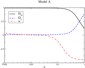
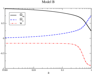
Figure 1: Evolution of matter and DE density parameters, $\Omega_{\rm m}\left(a\right)$ (solid black line) and $\Omega_{\rm de}\left(a\right)$ (blue dashed line), DE equation of state $w\left(a\right)$ (red dot-dashed line). Left (right) panel: Model A (B).

In Fig. 2 we also show the evolution of the comoving volume, given by

$$\frac{d^{2}V}{dzd\Omega}=\frac{r^{2}\left(z\right)}{H\left(z\right)}\,,$$ (2.5)

where $r\left(z\right)=\int_{0}^{z}H^{-1}\left(z^{\prime}\right)dz^{\prime}$. This quantity, which depends only on the background evolution is important for the study of cluster number counts, which in turn also depends on perturbative properties via the mass function. Note that both models of EDE that we are considering present a smaller volume then $\Lambda$CDM model and that important differences appear only at high$-z$. For redshifts $z<0.5$ all three volumes are very similar, which already suggests that cluster observations at low redshifts would poorly differentiate between these DE models. We will return to this issue in Sect. 5.

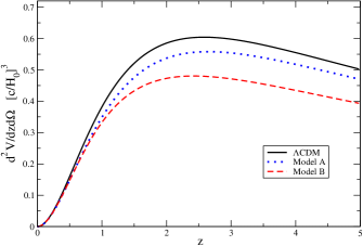
Figure 2: Comoving volume for $\Lambda$CDM model (solid black line) and models A (blue dotted line) and B (red dashed line) of EDE.

3 Linear evolution

In this section we study the linear relativistic evolution of a system with DE and matter. In models of EDE the energy density of DE at high redshifts, e.g., at the redshift of decoupling $z_{\rm dec}$, is not negligible, hence we carefully analyse approximate analytical solutions in order to establish consistent initial conditions for the equations of motion. Moreover this study will clarify some effects due to EDE and its perturbations.

In the Newtonian gauge, in Fourier space, in the absence of anisotropic stress, Ref. [39], the perturbed equations as a function of conformal time can be written as:

$$\dot{\delta}_{\rm m}+\theta_{\rm m}=3\dot{\phi}\;,$$ (3.1)

$$\dot{\theta}_{\rm m}+\mathcal{H}\theta_{\rm m}=k^{2}\phi\;,$$ (3.2)

$$\dot{\delta}_{\rm e}+3\mathcal{H}\left(\frac{\delta p_{\rm e}}{\delta\rho_{\rm e}}-w\right)\delta_{\rm e}+\left(1+w\right)\theta_{\rm e}=3\left(1+w\right)\dot{\phi}\;,$$ (3.3)

$$\dot{\theta}_{\rm e}+\mathcal{H}\left(1-3c_{\rm a}^{2}\right)\theta_{\rm e}=\frac{\left(\delta p_{\rm e}/\delta\rho_{\rm e}\right)k^{2}\delta_{\rm e}}{\left(1+w\right)}+k^{2}\phi\;,$$ (3.4)

$$k^{2}\phi+3\mathcal{H}\left(\dot{\phi}+\mathcal{H}\phi\right)=-\frac{3\mathcal{H}^{2}}{2}\left(\Omega_{\rm m}\delta_{\rm m}+\Omega_{\rm e}\delta_{\rm e}\right)\;,$$ (3.5)

where

$$c_{\rm a}^{2}=\frac{\dot{p}_{\rm e}}{\dot{\rho}_{\rm e}}=w-\frac{\dot{w}}{3\mathcal{H}\left(1+w\right)}$$ (3.6)

is the squared adiabatic sound speed and the pressure perturbation is given by [27]:

$$\delta p_{\rm e}=c_{{\rm eff}}^{2}\delta\rho_{\rm e}+3\mathcal{H}\left(1+w\right)\left(c_{{\rm eff}}^{2}-c_{\rm a}^{2}\right)\rho_{\rm e}\frac{\theta_{\rm e}}{k^{2}}\,.$$ (3.7)

Note that the equation of state can not cross the phantom barrier, otherwise $c_{\rm a}^{2}$ will diverge, and so will DE perturbations. In the two models we study there is no phantom crossing. For a treatment of this issue see Ref. [40]. We solve the system of equations (3.1)-(3.5) numerically, however the (ii)-Einstein equation, given by

$$\ddot{\phi}+3\mathcal{H}\dot{\phi}+\left(\frac{2\ddot{a}}{a}-\mathcal{H}^{2}\right)\phi=\frac{3\mathcal{H}^{2}}{2}\Omega_{\rm e}\left(\frac{\delta p_{\rm e}}{\delta\rho_{\rm e}}\right)\delta_{\rm e}\,,$$ (3.8)

will be useful to find analytical solutions.

It will also be useful to write a second order equation for the density contrast. For the sake of simplicity we assume that $c_{{\rm eff}}$ and $w$ are constants, then we have:

$$\ddot{\delta}+\left[\mathcal{H}\left(1-3w\right)-A\right]\dot{\delta}+\left[3\Delta\left(\dot{\mathcal{H}}+\mathcal{H}^{2}\right)-3\mathcal{H}\Delta A+c_{{\rm eff}}^{2}k^{2}\right]\delta=\left(1+w\right)\left(S-k^{2}\phi\right)\,,$$ (3.9)

where $\Delta=c_{{\rm eff}}^{2}-w$,

$$A=\frac{18\mathcal{H}\dot{\mathcal{H}}\Delta}{9\mathcal{H}^{2}\Delta+k^{2}}\,$$ (3.10)

and

$$S=3\ddot{\phi}+3\mathcal{H}\left(1-3c_{{\rm eff}}^{2}\right)\dot{\phi}-3A\dot{\phi}-9\mathcal{H}^{2}\Delta\phi\,.$$ (3.11)

Eq. (3.9) is valid for any perfect fluid characterised by constant $w$ and $c_{{\rm eff}}^{2}$, so the corresponding equation for matter is given by assuming $w=c_{{\rm eff}}^{2}=0$.

The function $A$ is related to the presence of the pressure perturbations that are proportional to $\theta$. It is useful to note that on small scales, $k\gg\mathcal{H}$, $A\simeq 0$ and $\delta p_{\rm e}\simeq c_{{\rm eff}}^{2}\delta\rho_{\rm e}$, as already observed in [41]. On large scales, $k\ll\mathcal{H}$, we have $A\simeq 2\dot{\mathcal{H}}/\mathcal{H}$ and the pressure perturbation strongly deviates from the value prescribed by $c_{{\rm eff}}$.

There are two important scales that determine the qualitatively behaviour of DE perturbations: the particle horizon

$$\lambda_{H}\left(a\right)=\int_{a_{i}}^{a}\frac{da^{\prime}}{a^{\prime}\mathcal{H}}\,,$$ (3.12)

(horizon for short), which is also important for matter perturbations, and the sound horizon

$$\lambda_{s}\left(a\right)=\int_{a_{\rm i}}^{a}\frac{c_{{\rm eff}}\left(a\right)da^{\prime}}{a^{\prime}\mathcal{H}}\,.$$ (3.13)

Perturbations with wavelength smaller than $\lambda_{s}$ oscillate with decreasing amplitude and eventually reach a minimum value proportional to the gravitational potential. Perturbations with wavelength larger than $\lambda_{s}$ effectively behave as pressureless, growing at the same pace as matter perturbations. Finally perturbations in both matter and DE with wavelength larger than $\lambda_{H}$ will follow the time dependence of the gravitational potential, being constant whenever DE effect in the background is negligible.

We are interested in small scales were nonlinear structures, such as galaxy clusters, form. Typically we can assume that the order of magnitude of such scales is $10\,\mbox{h}^{-1}\,\mbox{Mpc}$, or $k_{\rm nl}\simeq 0.63\,\mbox{h}\,\mbox{Mpc}^{-1}$. Shortly after decoupling, e.g., at $z=1000$, the horizon wave number is $k_{H}\simeq 0.017\,\mbox{h}\,\mbox{Mpc}^{-1}$ ($\Lambda$CDM with $\Omega_{\rm m}^{0}=0.25$ background is assumed), hence both DE and DM perturbations that go nonlinear are well inside the horizon on the onset of matter dominated period. For this reason we will focus our analysis on scales much smaller than $\lambda_{H}$, consequently the only scale important for DE perturbations is $\lambda_{s}$. For a study of scales larger than the horizon see Ref. [41].

It is interesting to determine the value of $c_{{\rm eff}}$, assumed constant, such that $k_{s}=k_{\rm nl}$ today:

$$c_{\rm nl}=9.4\times 10^{-4}\,.$$ (3.14)

In models with $c_{{\rm eff}}\ll c_{\rm nl}$ the sound horizon is always smaller than the nonlinear scale, then DE perturbations will behave as pressureless and we can effectively assume $c_{{\rm eff}}=0$. On the other hand, in models with $c_{{\rm eff}}\gg c_{\rm nl}$, DE perturbations are suppressed by its pressure support on nonlinear scales. In this work we treat the two limiting cases: one with negligible sound speed, $c_{{\rm eff}}=0$, and one with a non-negligible sound speed, $c_{{\rm eff}}=1$. For studies of time dependent $c_{{\rm eff}}$ in linear theory see Ref. [42] and for arbitrary values of $c_{{\rm eff}}$ during nonlinear evolution of DM see Ref. [43, 44].

3.1 Non-negligible $c_{{\rm eff}}$

On scales well inside the horizon, for constant $c_{{\rm eff}}$ and $w$, from Eq. (3.9), DE perturbations obey the following equation:

$$\delta_{e}^{\prime\prime}+\alpha\frac{\delta_{e}^{\prime}}{a}+\left(\beta+\frac{c_{{\rm eff}}^{2}k^{2}}{\mathcal{H}^{2}}\right)\frac{\delta_{e}}{a^{2}}=-\frac{\left(1+w\right)}{\mathcal{H}^{2}}\frac{k^{2}\phi}{a^{2}}\,,$$ (3.15)

where ${}^{\prime}=d/da$, $w_{\rm t}=\Omega_{\rm e}w$,

$$\alpha=\frac{3}{2}\left(1-w_{\rm t}\right)-3w\,,\,\,\,\,\,\mbox{and}\,\,\,\beta=\frac{3\Delta}{2}\left(1-3w_{\rm t}\right)\,.$$ (3.16)

Eq. (3.15) has the particular approximate solution:

$$\delta_{\rm e}\simeq-\frac{\left(1+w\right)\phi}{c_{{\rm eff}}^{2}}\,,$$ (3.17)

which becomes more accurate the bigger $c_{{\rm eff}}k/\mathcal{H}$ is. Note that since $c_{{\rm eff}}k/\mathcal{H}$ grows in time, as long as the background parameters do not change too fast in time, $\delta_{\rm e}$ will approach solution (3.17) on all scales. Moreover, the homogeneous solutions of Eq. (3.15) oscillate with decreasing amplitude [45, 41], hence eventually solution (3.17) will be reached and can be used to set the initial value of $\delta_{\rm e}$ as a function of $\phi$.

Before we determine the initial value of $\theta_{\rm e}$, we proceed to find solutions for $\phi$. Since we are interested on small scales we can assume that $\delta p_{\rm e}\simeq c_{{\rm eff}}^{2}\delta\rho_{\rm e}$. We verified that, for the IC we will determine and $c_{{\rm eff}}=1$, the error in this expression compared to Eq. (3.7) for a scale $k=0.1\mbox{h}\mbox{Mpc}^{-1}$ is initially of $1-3\%$ and below $1\%$ for $z<100$ and that the error decreases for smaller scales. Then, substituting the expression (3.17) in Eq. (3.8) and changing the independent variable to the scale factor $a$, the evolution of the gravitational potential is given by the equation:

$$\phi^{\prime\prime}+\left(\frac{7}{2}-\frac{3}{2}w_{\rm t}\right)\frac{\phi^{\prime}}{a}+\left(\frac{3\left(1+w\right)}{2}\Omega_{\rm e}-3w_{\rm t}\right)\frac{\phi}{a^{2}}=0\,.$$ (3.18)

This equation is valid as long as $\Omega_{\rm e}$ and $w$ are nearly constant, which is true for Model A roughly for $10<z<1000$ and for Model B roughly for $100<z<1000$. Solving this equation in this interval enables us to analytically evaluate the time variation of $\phi$. The solutions of Eq. (3.18) are power laws $\phi\propto a^{n}$, where $n$ is solution of the algebraic equation

$$n^{2}+\left(\frac{5}{2}-\frac{3}{2}w_{\rm t}\right)n+\frac{3\left(1+w\right)\Omega_{\rm e}}{2}-3w_{\rm t}=0\,.$$ (3.19)

For non-EDE models, when DE is very subdominant, we can set $\Omega_{\rm e}=0$ and the solutions are $n=0$ and $n=-2.5$, which indicates that, neglecting the decaying mode, the gravitational potential is constant during matter dominated era, a well known result for the Einstein-de-Sitter universe. However, in EDE models $\phi$ is not constant any more, its early time variation depends on both $\Omega_{\rm e}$ and $w$, but note it is independent of $c_{{\rm eff}}$.

The largest values of $n$, which give the solutions that decay more slowly, are

$$n_{\rm mod~{}A}=-0.0100\,\mbox{ and }\,n_{\rm mod~{}B}=-0.0127.$$ (3.20)

Since in Model A both $\Omega_{\rm e}$ and $w$ are approximately constant before DE domination, the error in this expression against the full numerical solution is below $1\%$ in the range $5<z<1000$. Given that in Model B the time variation of $\Omega_{\rm e}$ and $w$ is larger, its analytical solution has an error below $1\%$ only in the range $150<z<1000$.

Once we know how $\phi$ initially varies in time we can find $\dot{\delta}_{\rm e}$ from Eq. (3.17) and use Eq. (3.3) to determine the initial value of $\theta_{\rm e}$:

$$\theta_{\rm e}=3\dot{\phi}-\frac{\dot{\phi}}{c_{{\rm eff}}^{2}}-\frac{3\mathcal{H}\left(c_{{\rm eff}}^{2}-w\right)\phi}{c_{{\rm eff}}^{2}}\,.$$ (3.21)

Hence Eq. (3.21) can be used to determine the initial value of $\theta_{\rm e}$ as a function of the initial value of $\phi$ and its initial time derivative.

Finally we look for analytical solutions for matter perturbations in order to determine IC for $\delta_{\rm m}$ and $\theta_{\rm m}$. Setting $w=c_{{\rm eff}}=0$ in Eq. (3.15) we have:

$$\delta_{\rm m}^{\prime\prime}+\left(\frac{3}{2}-\frac{3w_{\rm t}}{2}\right)\frac{\delta_{\rm m}^{\prime}}{a}=-\frac{k^{2}\phi}{\mathcal{H}^{2}a^{2}}$$ (3.22)

It is useful to note that, although in EDE models $\Omega_{\rm e}$ is non-negligible at high-$z$, on small scales, since $\delta_{\rm e}\sim\phi$, we can assume that $\Omega_{\rm m}\delta_{\rm m}\gg\Omega_{\rm e}\delta_{\rm e}$ in Eq. (3.5), then we have:

$$\delta_{\rm m}\simeq\frac{-2k^{2}\phi}{3\mathcal{H}^{2}\Omega_{\rm m}}\,.$$ (3.23)

Using Eq. (3.23) we can find the initial value of $\delta_{\rm m}$ as a function of the initial value of a given $\phi$. Inserting Eq. (3.23) in Eq. (3.22) we have the equation for $\delta_{\rm m}$ alone:

$$\delta_{\rm m}^{\prime\prime}+\left(\frac{3}{2}-\frac{3w_{\rm t}}{2}\right)\frac{\delta_{\rm m}^{\prime}}{a}-\frac{3\Omega_{\rm m}}{2}\frac{\delta_{\rm m}}{a^{2}}=0\,,$$ (3.24)

which is the usual equation for the evolution of matter perturbations well inside the horizon. The solutions are power laws $\delta_{\rm m}\propto a^{p}$, where $p$ is determined by:

$$p^{2}+\left(\frac{1}{2}-\frac{3w_{\rm t}}{2}\right)p-\frac{3\Omega_{\rm m}}{2}=0\,.$$ (3.25)

Note that, under the approximations taken, when we compare Eqs. (3.25) and (3.19), we find that $n=p-1$. Then the corresponding values for $p$ are:

$$p_{\rm mod~{}A}=0.9900\,\,\,\mbox{and}\,\,\,\,p_{\rm mod~{}B}=0.9873\,.$$ (3.26)

In order to find the initial value of $\theta_{\rm m}$ we can use Eq. (3.1). The initial value of $\delta_{\rm m}$ and its initial dependence with $a$, is given by finding $p$ in Eq. (3.25). Then on small scales we have:

$$\theta_{\rm m}=-\dot{\delta}_{\rm m}\,.$$ (3.27)

In Fig. 3 we show the evolution of $\delta_{\rm e}$ according to the numerical solution of equations (3.1)$-$(3.5), and the analytical solution of Eq. (3.17), with $\phi$ given by the numerical solution. The only value we need to choose is $\phi_{i}=\phi\left(a_{i}\right)$, taking $a_{i}=0.001$ and $\phi_{i}=-6.2\times 10^{-6}$ we get $\delta_{m}\left(1\right)\simeq 0.1$. In order to check the consistency of the analytical solutions that we have used to determine the IC of DE perturbations, given by Eq. (3.17) and Eq. (3.21), (red dotted-dashed line) we also show the evolution of $\delta_{\rm e}$ using $\theta_{\rm e}$ ten times greater than as given by Eq. (3.21) (blue line). As we see, the solution of Eq. (3.17) is in good agreement with the numerical solution. In the case of bigger $\theta_{\rm e}$, $\delta_{\rm e}$ oscillates with an initial greater amplitude, which decreases with time and eventually approaches the value given by Eq. (3.17). For sake of clarity in these plots, we assumed $c_{{\rm eff}}^{2}=0.1$ in order to have a smaller frequency of oscillation. It is important to note that for this scale and for this value of $c_{\rm eff}$, at low $z$, DE perturbations are $4$ orders of magnitude smaller then $\delta_{m}$. For smaller scales and larger $c_{\rm eff}$, $\delta_{\rm e}$ will be even smaller than $\delta_{\rm m}$.

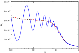
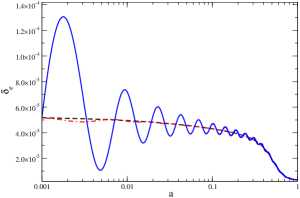
Figure 3: Linear evolution of $\delta_{\rm e}$ with $c_{{\rm eff}}^{2}=0.1$ for a mode $k=0.1\mbox{h}\mbox{Mpc}^{-1}$: analytical solution, Eq. (3.17) (black dashed line), numerical solution with IC from Eqs. (3.17) and (3.21) (red dot-dashed line) and the numerical solution with $\theta_{\rm e}$ ten times bigger (blue line). The change in the analytical solution due to the different IC is almost imperceptible in this scale so we only show the first case.

3.2 Negligible $c_{{\rm eff}}$

As we will see, in the case of negligible $c_{{\rm eff}}$, DE perturbations can have the same order of magnitude of matter perturbations. Although this fact impedes us to assume that $\Omega_{\rm m}\delta_{\rm m}\gg\Omega_{\rm e}\delta_{\rm e}$ for EDE models, fact that simplified the equations for the case of non-negligible $c_{{\rm eff}}$, when $c_{{\rm eff}}$ is negligible we will have another sort of simplification. Note that substituting the expression for the pressure perturbation, Eq. (3.7), in the equation for $\theta_{\rm e}$, Eq. (3.4), and assuming $c_{{\rm eff}}=0$ we obtain

$$\dot{\theta}_{\rm e}+\mathcal{H}\theta_{\rm e}=k^{2}\phi\,,$$ (3.28)

which is just the same equation for $\theta_{\rm m}$, Eq. (3.2). Hence both matter and DE perturbations will feel the same force and flow in the same way. Then, using Eqs. (3.1) and (3.3), we can determine an equation that directly relates $\delta_{\rm m}$ and $\delta_{\rm e}$:

$$\dot{\delta}_{\rm e}-3\mathcal{H}w\delta_{\rm e}=\left(1+w\right)\dot{\delta}_{\rm m}\,,$$ (3.29)

where, since, on small scales, both $\delta_{\rm m}$ and $\delta_{\rm e}$ will be of order $\mathcal{H}^{-2}k^{2}\phi$, we neglected the $\dot{\phi}$ term. Assuming that $\delta_{\rm m}\propto a^{p}$ we find the following relation between DE and matter perturbations:

$$\delta_{\rm e}=\frac{\left(1+w\right)p}{p-3w}\delta_{\rm m}\;.$$ (3.30)

In models with negligible amount of DE during matter era we have $p=1$, then

$$\delta_{\rm e}=\frac{\left(1+w\right)}{\left(1-3w\right)}\delta_{\rm m}\,,$$ (3.31)

which is in accordance with literature [45, 29, 46]. However, as we will show in Eq. (3.35), $p\simeq 1$ in EDE models with negligible $c_{{\rm eff}}$, then we can actually use Eq. (3.31) to set the initial value of $\delta_{\rm e}$ as a function of $\delta_{\rm m}$. It is also interesting to observe that Eq. (3.31) indicates that DE perturbations diverge as $w\rightarrow 1/3$, which can be achieved by a tracking scalar field during radiation dominated era. However this solution is valid only for $c_{{\rm eff}}=0$, hence, as consistency condition for DE perturbations, we should expect that whenever $w\rightarrow 1/3$ we must have $c_{{\rm eff}}>0$. In the models we are studying, during the matter dominated era and DE domination, we never have $w=1/3$.

At this point we derived a relation between DE and matter perturbations but not their evolution with time. Setting $w=c_{{\rm eff}}=0$ in Eq. (3.15) we have the equation for the evolution of $\delta_{\rm m}$:

$$\delta_{\rm m}^{\prime\prime}+\left(\frac{3}{2}-\frac{3w_{\rm t}}{2}\right)\frac{\delta_{\rm m}^{\prime}}{a}=\frac{3}{2a^{2}}\left(\Omega_{\rm m}\delta_{\rm m}+\Omega_{\rm e}\delta_{\rm e}\right)\,.$$ (3.32)

Now we can use Eq. (3.30) to express $\delta_{\rm e}$ as a function of $\delta_{\rm m}$ and rewrite Eq. (3.32) as

$$\delta_{\rm m}^{\prime\prime}+\left(\frac{3}{2}-\frac{3w_{\rm t}}{2}\right)\frac{\delta_{\rm m}^{\prime}}{a}-\frac{3}{2}\left(\Omega_{\rm m}+\frac{\left(1+w\right)p}{p-3w}\Omega_{\rm e}\right)\frac{\delta_{\rm m}}{a^{2}}=0\,.$$ (3.33)

While $\Omega_{\rm m}$, $\Omega_{\rm e}$ and $w$ are nearly constants we can find the solution $\delta_{\rm m}\propto a^{p}$, where $p$ is solution of

$$p^{2}+p\left(\frac{1}{2}-\frac{3w_{\rm t}}{2}\right)-\frac{3}{2}\left(\Omega_{\rm m}+\frac{\left(1+w\right)p}{p-3w}\Omega_{\rm e}\right)=0\,.$$ (3.34)

For the two models we are studying we have the following values at $a_{i}$:

$$p_{\rm mod~{}A}=1.0052\,\,\,\mbox{and}\,\,\,\,p_{\rm mod~{}B}=0.9934\,.$$ (3.35)

As we can see, the deviation from $p=1$ is very small and we could actually use expression (3.31) in order to determine the initial value of $\delta_{\rm e}$ as a function of $\delta_{\rm m}$. Moreover expression (3.31) gives a better order of magnitude estimation of $\delta_{\rm e}$ for low$-z$ than Eq. (3.30), that depends on the determination of $p$ from Eq. (3.34), which is not accurate for low$-z$, when both $\Omega_{\rm e}$ and $w$ can not be assumed constant. Hence in what follows we will use the expression (3.31) to compute the initial value of the DE perturbation.

To determine the initial value of $\delta_{\rm m}$ as a function of $\phi$ we use Eq. (3.30) in Eq. (3.5), then, for small scales we have:

$$\delta_{\rm m}=-\frac{2k^{2}\phi}{3\mathcal{H}^{2}\left(\Omega_{\rm m}+\Omega_{\rm e}\frac{1+w}{1-3w}\right)}\,.$$ (3.36)

The initial value of $\theta_{\rm m}$ can be determined in the same way as we did for the case of non-negligible $c_{{\rm eff}}$, using Eq. (3.27).

Now we proceed to find the initial time variation for $\phi$. For the case $c_{{\rm eff}}=0$ DE perturbations do not contribute to the variation of $\phi$, i.e., the RHS of Eq. (3.8) is zero and then the equation that determines the power of $n$ of $\phi$ is the following:

$$n^{2}+n\left(\frac{5}{2}-\frac{3}{2}w_{\rm t}\right)-3w_{\rm t}=0\,.$$ (3.37)

Here, in contrast to the case of non-negligible $c_{{\rm eff}}$, the relation $n=p-1$ is not valid. Note also that $n$ only depends on the product $\Omega_{\rm e}w$, differently from case of non-negligible $c_{{\rm eff}}$, where it also depends directly on $\Omega_{\rm e}$. This indicates that EDE models with negligible sound speed give a very low contribution to the time variation of $\phi$, due to the fact that, although $\Omega_{\rm e}$ is not negligible during the matter era, we have $\Omega_{\rm e}w\simeq 0$. The highest values of $n$ for models A and B are:

$$n_{\rm mod~{}A}=0.0017\,\,\,\mbox{and}\,\,\>n_{\rm mod~{}B}=-0.0036\,.$$ (3.38)

Note that the absolute value of $n$ is one order of magnitude smaller than the solutions for the case of non-negligible $c_{{\rm eff}}$, Eq. (3.20). Since the background evolution is the same for both cases, this clearly shows that the most important effect for the evolution of the gravitational potential in EDE models is pressure perturbation.

In Fig. 4 we show the evolution of matter and DE perturbations as well as the evolution of $\delta_{\rm e}$ according to Eq. (3.31). We show this relation, instead of the more general one, in Eq. (3.30), because initially the deviation from $p=1$ is very small (bellow $1\%$) and for late times, when $\Omega_{\rm m}$, $\Omega_{\rm e}$ and $w$ are not constant, the computation of $p$ via Eq. (3.34) is less accurate than just assuming $p=1$. As we can see, Eq. (3.31) is a very good approximation for $\delta_{\rm e}$ during the matter dominated era, however, once the transition to the DE dominated era starts, it becomes much less accurate. Anyhow Eq. (3.31) can be used as an estimate of the order of magnitude of $\delta_{\rm e}$ for late times. It is also interesting to note that in Model A the perturbations in DE are larger than matter perturbations until $w$ starts to decrease, $a\simeq 0.1$. For Model B, since $1+w$ is smaller than in Model A, $\delta_{\rm e}$ is smaller during most of the evolution. However, due to the latter transition of $w$ in Model B, $\delta_{\rm e}$ starts to decrease at a later time and its final value is larger then in Model A.

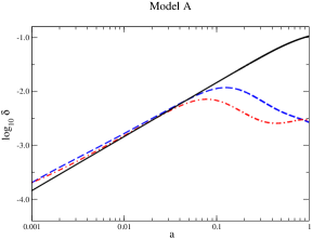
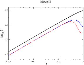
Figure 4: Linear evolution of perturbations with $c_{{\rm eff}}=0$ and $k=0.1\mbox{h}\mbox{Mpc}^{-1}$: numerical solution of $\delta_{\rm m}$ (black solid line), numerical solution of $\delta_{\rm e}$ (blue dashed line) and $\delta_{\rm e}$ according to the relation given by the analytical solution, Eq. (3.31), (red dot-dashed line).

3.3 Matter growth and ISW effect

Once we know approximate analytical solutions to set the IC of the system of equations, we proceed to study the effects of EDE models on the linear evolution of matter perturbations and gravitational potential.

In Fig. 5 we show the evolution of the normalised growth function $D/a$, where $D=\delta_{\rm m}\left(a\right)/\delta_{\rm m}\left(1\right)$, and the logarithmic derivative of the growth function $f=d\mbox{ln}D/d\mbox{ln}a$ and its percentual difference against $\Lambda$CDM,

$$\Delta f=100\times\frac{f_{\rm mod}-f_{\Lambda CDM}}{f_{\Lambda CDM}}\,.$$ (3.39)

In the $\Lambda$CDM model, both the normalised growth and $f$ tend to a constant value for low $a$ (high $z$) because $D\rightarrow a$ whenever DE is very subdominant. In this limit $f\rightarrow 1$ and $D/a\rightarrow 1.34$.

In EDE models $D/a$ and $f$ vary at high $z$, but in the case of $c_{{\rm eff}}=0$, DE perturbations tend to compensate the change in background evolution due to EDE and their values get closer to the $\Lambda$CDM values. In the case of $c_{{\rm eff}}=1$, DE perturbations are much smaller and practically do not compensate the change in the background evolution, thus the deviation from $\Lambda$CDM is more prominent.

This behavior can be clearly understood in terms of Eqs. (3.24) and (3.32). For a given model, when $c_{{\rm eff}}=0$, DE perturbations enhance DM clustering via the last term in the LHS of Eq. (3.32), which is absent in Eq. (3.24). Since EDE models have a less decelerated background expansion than $\Lambda$CDM model during the matter dominated era, which in turn makes DM clustering less efficient, the contribution of DE perturbations in the case of $c_{{\rm eff}}=0$ tend to compensate this change, making DM growth in these models more similar to the $\Lambda$CDM one at high $z$.

At low $z$ the situation is reversed, EDE models show a less accelerated expansion, which induces a faster DM growth than in $\Lambda$CDM. Again DE perturbations enhance this growth, but now making it more different from the $\Lambda$CDM one. Therefore, as we can see in Fig. 5, $\Delta f$ becomes larger at low $z$, particularly for EDE models with $c_{{\rm eff}}=0$. Note that this effect is more important in Model B, which presents larger DE perturbations at low $z$. However, the integrated impact of DE perturbations, which can be observed via $D/a$ at $a=0.001$, always makes DM growth more similar to $\Lambda$CDM. As we will see in Sect. 5 the integrated impact of EDE models in DM growth will cause large differences in the abundance of galaxy clusters via the normalisation of the matter power spectrum, $\sigma_{8}$, but the specific influence of DE pertubations is to make cluster abundace more similar to the predictions of $\Lambda$CDM model.

Besides this general behaviour of EDE models, we can see that Model B produces the most distinct evolution and variation between the two values of $c_{{\rm eff}}$. This is mainly caused by the rapid transition of its equation of state, which produces a very different background evolution and also allows DE perturbations to grow for a longer period when $c_{{\rm eff}}=0$. Although the background evolution of Model B may be unrealistic, for instance, providing a rather low age of $13.01\,$Gy, it is very valuable to clearly identify the changes that large DE perturbations may cause. Since current data on $f$ have a precision around $10\%$ [5], even in Model B, large DE perturbations would be weakly distinguished from the case of negligible DE fluctuations. However future surveys like Euclid, which may achieve about $1\%$ precision [47], could make a much more significant distinction.

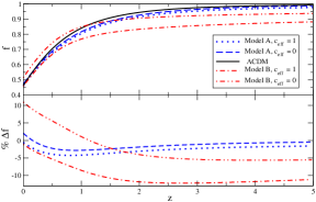
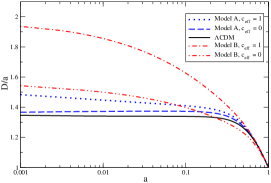
Figure 5: Evolution of $f$ (left top panel), its percentage difference against $\Lambda$CDM model (left bottom panel) and the normalised growth factor $D/a$ (right panel), for a mode $k=0.1\mbox{h}\mbox{Mpc}^{-1}$. Line styles and colours for the different models are indicated in the legends.

The Sachs-Wolfe effect [48] causes the gravitational blueshift (redshift) of CMB photons when they fall in (escape from) potential wells near the time of last scattering. When the gravitational potential varies in time, the temperature variation of CMB photons is associated with the Integrated Sachs-Wolfe effect (ISW). Assuming zero opacity the temperature fluctuation is proportional to:

$$\frac{\Delta T}{T}\propto\int_{\eta_{0}}^{\eta_{\rm dec}}\dot{\phi}d\eta=\phi\left(\eta_{\rm dec}\right)-\phi\left(\eta_{0}\right)\,,$$ (3.40)

where $\eta_{\rm dec}$ and $\eta_{0}$ are the conformal time at decoupling $\left(z_{\rm dec}\simeq 1100\right)$ and now, respectively. The ISW effect can be separated into two components: the early ISW, which is usually attributed to the influence of residual radiation energy after the redshift of last scattering and the late ISW, associated with the accelerated expansion at low redshift. Since we neglect radiation, we will only deal with ISW originated by DE. While $\Omega_{\rm m}\simeq 1$, the gravitational potential is nearly constant on all scales and the corresponding ISW during matter dominated era is negligible. However, for EDE models we have $\Omega_{\rm m}\simeq 0.99$ at high$-z$, so the background evolution alone should generate a distinct time evolution for $\phi$. Moreover, pressure perturbations in EDE directly source the time variation of the gravitational potential, Eq. (3.8), and it turns out that this contribution is more important. In order to visualise how EDE and its perturbations generate the ISW effect, in Fig. 6 we show the function

$$F=\frac{\phi\left(a\right)}{\phi\left(a_{dec}\right)}\,,$$ (3.41)

so we have $\frac{\Delta T}{T}\propto\phi\left(a_{\rm dec}\right)\left(1-F\left(1\right)\right)$. One can clearly see that the time variation of $\phi$ is greater in models with $c_{{\rm eff}}=1$ than $c_{{\rm eff}}=0$. Since the background evolution of Model A is similar to $\Lambda$CDM, in the case of $c_{{\rm eff}}=0$ the ISW effect is also very similar to the $\Lambda$CDM model. Again, the general effect of models with null $c_{{\rm eff}}$ is to compensate the changes of EDE in the background evolution. Although in principle ISW has limited power to constrain DE models due to its large cosmic variance, the observation of this effect is improving and a detection of $4.4\sigma$ level has been reported [49].

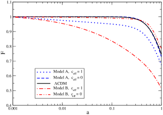
Figure 6: Evolution of the function $F$, Eq. (3.41), as a function of the scale factor. The curve of Model A with $c_{{\rm eff}}=0$ is almost indistinguishable from $\Lambda$CDM model.

4 Nonlinear evolution

Now we proceed to study the nonlinear evolution of DE and matter fluctuations, which can provide important information about the formation of DM halos. One difficulty that arises in this analysis is how to evolve DE fluctuations in the nonlinear regime. Many authors have addressed this issue using the Spherical Collapse Model, e.g., [50, 51, 52, 46, 43]. Independently of the approach used, the most important point we have to observe is when DE fluctuations actually become nonlinear, i.e., $\delta_{e}\gtrsim 1$. The key property that controls this behaviour is the effective sound speed, $c_{{\rm eff}}$, which was shown can be constrained using future data on the abundance of galaxy clusters [53, 44].

As we showed in the linear regime, DE perturbations in models with non-negligible $c_{{\rm eff}}$ are at least few orders of magnitude smaller than $\delta_{\rm m}$ on small scales. We also verified that, in this case, neglecting DE perturbations changes the value of the linearly evolved $\delta_{\rm m}$ only about $0.02\%$. Moreover its value is proportional to the value of $\phi$, which, before DE domination, is known to remain approximately constant even during the nonlinear regime [54, 55]. Hence we expect that the contribution of $\delta_{\rm e}$ for the gravitational potential will be very small during the nonlinear regime. For this reason, in the case of $c_{{\rm eff}}=1$, we assume that DE perturbations can be neglected for the nonlinear evolution.

For the case of $c_{{\rm eff}}=0$, DE perturbations can have the same order of magnitude of matter perturbations, hence they can not be neglected, otherwise the linearly evolved $\delta_{\rm m}$ can change up to $20\%$. Evidently an intermediate behaviour should appear when $c_{{\rm eff}}\gtrsim c_{\rm nl}$, in this case one could incorporate the linear evolution DE perturbations with the nonlinear evolution of DM [43]. Here we want to focus on the two limiting cases: the one where $\delta_{\rm e}$ is most unimportant for the nonlinear evolution of DM, $c_{{\rm eff}}=1$, and the other where $\delta_{\rm e}$ is the most important for it.

We use the fluid approach to solve the SC model derived from the Pseudo-Newtonian Cosmology (PNC) [52, 45], which is suitable to treat the nonlinear evolution of perfect fluids with relativistic pressure on small scales. The equations for a system with matter and DE fluctuations, with $c_{{\rm eff}}=0$, can be written as:

$$\dot{\delta}_{\rm m}+\theta\left(1+\delta_{\rm m}\right)=0\,,$$ (4.1)

$$\dot{\delta}_{\rm e}-3\mathcal{H}w\delta_{\rm e}+\theta\left(1+w+\delta_{\rm e}\right)=0\,,$$ (4.2)

$$\dot{\theta}+\mathcal{H}\theta+\frac{\theta^{2}}{3}=-\frac{3\mathcal{H}^{2}}{2}\left(\Omega_{\rm m}\delta_{\rm m}+\Omega_{\rm e}\delta_{\rm e}\right)\,.$$ (4.3)

For the case of negligible DE perturbations we only need to evolve Eqs. (4.1) and (4.3), setting $\Omega_{\rm e}\delta_{\rm e}=0$ in the latter, in this case we have the usual SC model for dark matter [56, 57, 58].

The most relevant quantity we compute using the SC model is the critical density contrast, $\delta_{\rm c}$, defined by

$$\delta_{\rm c}\left(z_{\rm c}\right)=\delta_{\rm mL}\left(z_{\rm c}\right)\,,$$ (4.4)

where $\delta_{\rm mL}$ is the linearly evolved matter density contrast with initial conditions such that non-linearly evolved $\delta_{\rm m}$ has vertical asymptote at $z_{\rm c}$, i.e.,

$$\underset{z\rightarrow z_{\rm c}^{+}}{\lim}\delta_{\rm m}\left(z\right)=\infty\,.$$ (4.5)

Numerically we need to determine some value above which we consider $\delta_{\rm m}$ has diverged; we observed that choosing $10^{5}$ gives the classical value in Einstein-de-Sitter universe, $\delta_{\rm c}\simeq 1.686$, with an error of at most $0.5\%$ for $0\leq z\leq 4$.

The function $\delta_{\rm c}$ depends both on the linear and nonlinear evolution. Although we do not have a framework to solve the relativistic SC model, we can compare the PNC and GR predictions for the linear evolution. It is clear that PNC will not give accurate results for scales of order of magnitude comparable with the horizon, however, for $k=0.1\,\mbox{h}\,\mbox{Mpc}^{-1}$, the values of $\delta_{\rm m}$ given by PNC differ from GR at most $0.1\%$ and decreases for smaller scales. Hence computing $\delta_{\rm c}$ using Eqs. (4.1)$-$(4.3) and its linearised version should be a good approximation.

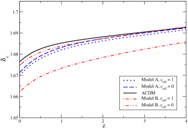
Figure 7: Evolution of $\delta_{\rm c}\left(z_{\rm c}\right)$ for the different models. Line styles and colour are shown in the legend box.

Now we need to provide the initial conditions to evolve the nonlinear equations. We choose values of $\delta_{\rm m}\left(a_{\rm i}\right)$ in order to get $0\leq z_{c}\leq 4$. As we discussed in section 3.2, for the case of null $c_{{\rm eff}}$ we can determine $\delta_{\rm e}\left(a_{\rm i}\right)$ using Eq. (3.31), use $\theta\left(a_{\rm i}\right)=-\dot{\delta}_{\rm m}\left(a_{\rm i}\right)$, assuming $\delta_{\rm m}\propto a$. For the case of non-negligible $c_{{\rm eff}}$ we assume $\delta_{\rm m}\propto a^{p}$ with $p$ determined by Eq. (3.26). It is important to observe that all these relations can be derived from the PNC equations, Eqs. (4.1)$-$(4.3).

We show the critical density contrast in function of $z$ in Fig. 7. For the cases of $c_{{\rm eff}}=0$ DE perturbations clearly make $\delta_{\rm c}$ closer to the $\Lambda$CDM values. This happens because, while at background level EDE changes the expansion rate and lowers $\Omega_{\rm m}$, DE perturbations contribute to the gravitational potential, compensating the change in background. Note that the values of $\delta_{\rm c}$ that we found are consistent with small departures (less than $1\%$) from $\Lambda$CDM values [59, 34], even in the presence of large EDE fluctuations.

The total mass of halos

In models with clustering DE we must care about its contribution to the total mass of the halo. The presence of DE can either add or subtract mass from the forming DM halo. For the case of negligible $c_{{\rm eff}}$, Ref. [46] argues that DE contribution is constant in time and evaluates it at the virialization radius, $R_{\rm vir}$.

The computation of $R_{\rm vir}$ depends on the details of the virialization process. In the usual SC model, in an EdS universe, the virialization radius is half of the turnaround radius, $R_{\rm vir}=R_{\rm ta}/2$. Once the virialization is reached one can define the DM overdensity of the formed halo. There are two common definitions: $\Delta_{\rm V}(z_{\rm c})=(\rho_{m}(z_{\rm v})+\delta\rho_{\rm m}(z_{\rm v}))/\rho_{m}(z_{\rm c})\simeq 178$, where $z_{\rm v}$ is the redshift of virialization, and $\Delta_{\rm V}(z_{\rm v})=(\rho_{m}(z_{\rm v})+\delta\rho_{\rm m}(z_{\rm v}))/\rho_{m}(z_{\rm v})\simeq 147$, see Refs. [60, 61] for details and discussion. However when DE is present these values change in time and the virialization process also depends on the properties of DE [62, 63, 46, 44].

Here we will use the usual relation between turn-around and virialization radius $R_{\rm vir}=R_{\rm ta}/2$. Although this is not valid in non-EdS models and the values of $\Delta_{\rm V}$ can be considerably different, this simplified relation gives a good approximation for the fraction of DE mass to the DM mass:

$$\epsilon=\frac{M_{\rm e}}{M_{\rm m}}\,.$$ (4.6)

For instance, we checked that changing $R_{\rm vir}$ by $5\%$, which is common for inhomogeneous DE models Ref. [43], changes $\epsilon$ by $1\%$.

After solving the system of Eqs. (4.1)$-$(4.3) we find the value $R$ using the conservation of DM mass:

$$\delta_{\rm m}+1=(\delta_{\rm m_{\rm i}}+1)\left(\frac{a}{a_{\rm i}}\frac{R_{\rm i}}{R}\right)^{3}\;.$$ (4.7)

The virialized mass associated with DM is then given by:

$$M_{\rm m}=4\pi\int_{0}^{R_{vir}}dRR^{2}(\rho_{\rm m}+\delta\rho_{\rm m})\,.$$ (4.8)

Now we also have to define the DE mass contained in the same region where the DM halo has been formed, $M_{\rm e}$. In Ref. [46] it is defined as the matter associated only with the fluctuations of DE, which we will call

$$M_{\rm e_{\rm P}}=4\pi\int_{0}^{R_{vir}}dRR^{2}\delta\rho_{\rm e}\,.$$ (4.9)

However, this choice makes a discrimination between the DE and DM contributions. The latter is computed using its total density, $\rho_{\rm m}+\delta\rho_{\rm m}$, whereas the former only considers the fluctuation contribution. Treating the two fluids on equal foot, the total contribution of DE mass can be evaluated based on the so-called active density in the Poisson equation in the presence of relativistic pressure, $\nabla^{2}\phi=4\pi G(\rho+3p)$. Hence we have:

$$M_{\rm e_{\rm T}}=4\pi\int_{0}^{R_{vir}}dRR^{2}\left[(1+3w)\rho_{\rm e}+(1+3c^{2}_{{\rm eff}})\delta\rho_{\rm e}\right]$$ (4.10)

The motivation to consider the total mass (background plus perturbative contributions) is that the astrophysical processes associated with galaxy clusters are sensitive to the total gravitational potential. This interpretation is also carried out by Ref. [64] in order to estimate the mass of the Local Group. Although this background contribution may be debatable we decided to evaluate it in order to verify whether it can produce a non-negligible effect. For models with $c_{{\rm eff}}=1$, DE perturbations are much smaller than unity at the virialization time, hence they can be neglected in Eq. (4.10).

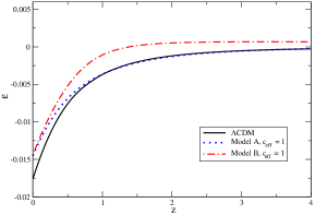
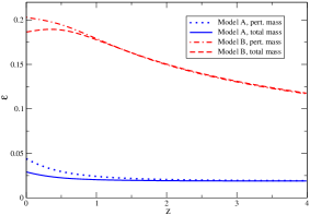
Figure 8: Evolution of $\epsilon(z)$. Left panel: $\Lambda$CDM model and models A and B with $c_{\rm eff}=1$. Right panel: Model A only with perturbation contribution (dotted blue line) and total contribution (solid blue line), Model B only with perturbation contribution (dot-dashed red line) and with total contribution (dashed red line), all with $c_{\rm eff}=0$.

In Fig. 8 we show the evolution of the quantity $\epsilon$ for models with homogeneous DE (left panel), in which case we compute $\epsilon$ using Eq. (4.10), and for models with inhomogeneous DE, computing $\epsilon$ both with Eq. (4.9) and Eq. (4.10) (right panel). Note that due to the background contribution in Eq. (4.10), even in the case of $c_{{\rm eff}}=1$ and $\Lambda$CDM models, DE can subtract only about $1\%$ of DM mass. However this effect appears only at low redshifts, when $\Omega_{\rm e}\sim\Omega_{\rm m}$. For the case of $c_{{\rm eff}}=0$, the fraction of DE in a DM halo can be much larger, but now adding mass to the halo. In these models the DE contribution does not go to zero at higher $z$ because of the combination of two factors: while $\Omega_{\rm e}$ decreases, but not to negligible values, $w$ decreases as well, which in turn, according to Eq. (3.31), makes the ratio $\delta_{\rm e}/\delta_{\rm m}$ grow.

This is a characteristic behaviour of EDE models. As already shown in Ref. [46], for the perturbative contribution and constant $w$, around $-1$, $\epsilon$ is at most $0.05$ and tends to zero as $z$ grows. In Ref. [44], for models with $w=-0.8$ and $c_{{\rm eff}}^{2}=10^{-6}$, the authors claim that maximal value of DE mass fraction in halos is $0.1\%$. However they assume DE fluctuations are small and can be treated within linear theory, which is not valid for the models with $c_{{\rm eff}}=0$ we are studying.

5 Abundance of halos

In this section we study the effect DE fluctuations on the abundance of halos. We decided to parametrize the mass function using the Sheth & Tormen (ST) prescription [65, 66, 67]:

$$\frac{dn}{dM}=-\sqrt{\frac{2a}{\pi}}A\left[1+\left(\frac{a\delta_{c}^{2}}{D^{2}\sigma^{2}_{M}}\right)^{-p}\right]\frac{\bar{\rho}_{m}}{M^{2}}\frac{\delta_{c}}{\sigma_{M}}\frac{d\ln\sigma_{M}}{d\ln M}\exp\left(\frac{-a\delta_{c}^{2}}{2D^{2}\sigma^{2}_{M}}\right)\,$$ (5.1)

where $a=0.707$, $p=0.3$, $A=0.2162$,

$$\sigma^{2}_{M}=\frac{1}{2\pi^{2}}\int_{0}^{\infty}dkk^{2}W^{2}\left(kR\right)P(k)$$ (5.2)

is the squared variance of the matter power spectrum, P(k), which we computed using the BBKS transfer function [68], smoothed with a top-hat window function, $W(kR)=3(kR)^{-3}(\sin(kR)-kR\cos(kR))$, where $R$ is the scale enclosing the mass $M=(4\pi/3)R^{3}\bar{\rho}_{m}$ and $\bar{\rho}_{\rm m}$ is the comoving matter density. The ST mass function depends critically on the linear overdensity parameter $\delta_{\rm c}$ of dark matter, therefore also a small variation of this quantity will give a huge effect on the high-mass tail of the mass function.

In order to clearly observe the effects of DE fluctuations we compute the number density of objects above a given mass at fixed redshift:

$$n(>M)=\int_{M}^{\infty}\frac{dn}{dM^{\prime}}dM^{\prime}\;.$$ (5.3)

We choose four different redshifts, namely $z=0,0.5,1,2$. The actual number of halos also depend on a integral over the comoving volume, hence it depends both on background and perturbative properties of DE. For the models we consider the comoving volume is always smaller than in $\Lambda$CDM, see Fig. 2.

We adopt as reference model the $\Lambda$CDM model with normalisation of the matter power spectrum $\sigma_{8}=0.776$, in agreement with CMB measurements by the WMAP team [69, 70]. Since the background history and therefore the growth factor for the EDE models differ from the $\Lambda$CDM models, perturbations will evolve differently in the different classes of models. Therefore we decide to adopt the CMB normalisation: we fix the same amplitude of the perturbations at the CMB epoch and we rescale it by the ratio of the different growth factors. More quantitatively we have

$$\sigma_{8,\rm DE}=\sigma_{8,\Lambda\rm CDM}\frac{D_{\Lambda\rm CDM}(z_{\rm dec})}{D_{\rm DE}(z_{\rm dec})}\;.$$ (5.4)

In Tab. 1 we show the normalisation of the power spectrum for the dark energy models considered in this work.

Table 1: Table of the normalisation of the matter power spectrum for the different models analysed.

Model	$\sigma_{8}$
A, $c_{\rm eff}=0$	0.761
A, $c_{\rm eff}=1$	0.698
B, $c_{\rm eff}=0$	0.674
B, $c_{\rm eff}=1$	0.532

As one can notice, the Model B is the one differing most from the $\Lambda$CDM model. The matter power spectrum normalisation when $c_{\rm eff}=1$ is 30% lower than the reference, therefore we expect that the mass function will be significantly different from the reference $\Lambda$CDM model. In Fig. 9 we show the ratio between the number density of dark matter halos for the EDE models and the $\Lambda$CDM model. We refer to the caption for the different line-styles and colours.

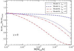
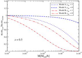
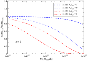
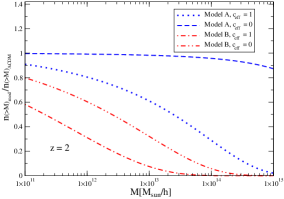
Figure 9: Number density ratio between the EDE models and the reference $\Lambda$CDM model. The red dashed (blue short-dashed) curve shows results for Model A with $c_{\rm eff}=0$ ($c_{\rm eff}=1$), while the cyan dotted (orange dot-dashed) curve represents Model B for $c_{\rm eff}=0$ ($c_{\rm eff}=1$). The upper left (right) panel shows results for $z=0$ ($z=0.5$), while the lower left (right) panel shows results for $z=1$ ($z=2$).

It is immediately clear that for Model B structures are strongly suppressed at all redshifts with respect to the $\Lambda$CDM model. Model B shows a lack of objects already at galactic scales ($M\simeq 10^{11}-10^{12}~{}M_{\odot}/h$) while at cluster scales ($M~{}\approx 10^{15}~{}M_{\odot}/h$) the case with $c_{\rm eff}=1$ has basically no objects (see the upper left panel). At higher redshifts, the number of objects decreases considerably also at very low scales (see lower right panel for the results at $z=2$).

Model A suppresses structures less than Model B and for low mass objects at $z=0$ the Model A with $c_{\rm eff}=1$ is quite similar to the Model B with $c_{\rm eff}=0$, but for masses of the order of $10^{15}~{}M_{\odot}/h$ they differ by about $30\%$. With the increase of the redshift, differences between the two models of EDE tend to increase. The most similar model to the $\Lambda$CDM one is Model A with $c_{\rm eff}=0$. Also at very high masses differences are at most about $20\%$. It is also important to bear in mind that the actual number of halos will also depend on the comoving volume, Fig. 2, which for EDE models is always smaller than in $\Lambda$CDM models. For low redshifts, $z=0$ and $z=0.5$, the differences in the comoving volume is very small, but for $z=1$ and $z=2$ the actual number of halos in EDE models will be even smaller than the ratios in the lower panels of Fig. 9 suggest.

It is also worth to note that models with $c_{\rm eff}=0$ have more objects than the case with $c_{\rm eff}=1$. This is easily explained in terms of the growth factor and of the evolution parameter $\delta_{\rm c}$. Again the general effect of large DE fluctuations is to compensate the change in the background evolution by enhancing the gravitational attraction.

The contribution of DE mass to the mass functions

As already observed in Ref. [46], if DE can cluster it also contributes to the halo mass, thus we must compute the correction to the mass function due to this extra component. The actual contribution of DE crucially depends on whether it virializes and the time scale of this process. Moreover the merging history of halos formed at different times [71], which could contain different amounts of DE, should also be taken into account. A complete and accurate description of this corrections is a complex task, which depends on nature of DE, and is beyond the scope of this paper. Here we will compute a straightforward correction for a scenario where, in the case of $c_{\rm eff}=0$, we assume that DE virializes together with DM on the same time scale. Hence, once the halo is formed, DE contribution is assumed to remain constant. This is probably the case in which DE fluctuations will mostly influence structure formation and consequently the mass function.

Given a halo with DM mass $M$, its total mass will be $M(1+\epsilon(z))$, with $\epsilon(z)$ defined in Eq. (4.6). Therefore, given the original DM mass function, $\frac{dn}{d\ln{M}}$, we assume the corrected mass function is given by:

$$\frac{dn_{c}}{d\ln{M}}(z,M)=\frac{dn}{d\ln{M}}\left(z,M(1-\epsilon)\right)\;.$$ (5.5)

We call the attention of the reader to the minus sign in $M(1-\epsilon)$. Although the mass of a halo is changed by $M\rightarrow M(1+\epsilon)$ the use of this mass redefinition in the mass function would produce wrong results. For a positive $\epsilon$ the halos become more massive than predicted by a model in which only DM clusters, hence more massive halos are expected. However, if one redefines the mass function using $M(1+\epsilon)$, fewer massive halos would be predicted, which is just the opposite of what is expected. Therefore the natural correction of the mass function is the change of variable $M\rightarrow M(1-\epsilon)$.

In Fig. 10 we show how much is the correction in the comoving density of objects above mass $M$ relative to the same model without the correction, $n_{c}(>M)/n(>M)$. We present the results for models A and B, with $c_{\rm eff}=0$, only for the perturbative contribution (top panels). Although it is not clear whether the background energy density of DE is a stable contribution to the total mass of the halo, i.e., that is constant through the history of the halo, in order to have an idea of its influence on the abundance of halos, we also show the corrections due to the background contribution in the $\Lambda$CDM model (bottom panel).

As can be seen in the these three cases, it is clear that even a small DE contribution for the halo mass can produce drastic changes at high mass. For Model B, the one with largest $\epsilon$, $n_{c}$ can be many times larger then its version without the mass correction. In Model A the corrections are below $10\%$ for small masses but can reach almost $60\%$ for high masses at high $z$. For $\Lambda$CDM, the corrections can be about $3\%$ at $z=0$ and low masses, reaching more than $10\%$ for very massive halos at high $z$.

It is also clear that, although $\epsilon$ gets smaller at higher $z$, the corrections do not necessarily diminish, as can be seen for the three cases with $z=2$. Since the growth function, $D$, gets smaller for high $z$, the exponential decay of the mass functions is shifted to lower mass regions, hence even a small value of $\epsilon$ at high $z$ produces large modifications. The comprehension of this effect is very important because, despite the fact that very few massive galaxy clusters are expected at high $z$, the detection of a single massive distant galaxy cluster can be used to rule out DE models [72].

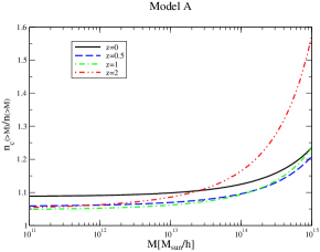
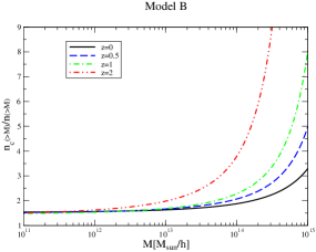
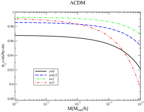
Figure 10: Ratio of comoving number density above mass $M$ at fixed redshifts, computed with the mass function correction, Eq. (5.5), $n_{c}(>M)$ to the comoving number density in the same model without the correction $n(>M)$. In Model B the corrections reach $60$ times at $z=2$.

Now that we observed that the corrections in mass functions can be important, we have to ask ourselves whether they can change the behaviour that we previously found without taking into account such corrections, i.e., that all EDE models we consider have smaller density of objects then $\Lambda$CDM, Fig. 9. In Fig. 11 we plot the ratio of the corrected values of number density, $n_{c}$, to the $n$ in $\Lambda$CDM model. For small masses, the corrections indicate that our inhomogeneous EDE models actually present more objects than $\Lambda$CDM. However, $n_{c}(>M)/n(>M)_{\Lambda CDM}$ decreases with mass, except for Model A at $z=2$. For Model B the suppression of structures due to its low $\sigma_{8}$ value is so strong that, even with the large corrections caused by its large values of $\epsilon$, at high masses it always has fewer objects density than $\Lambda$CDM.

In Model A a quite interesting behaviour can be observed. Since its $\sigma_{8}$ and growth function are not very different than in $\Lambda$CDM, the correction due to DE mass turns out to be more important at high $z$ and rapidly increases with mass. At $z=2$ the number density in Model A is about $36\%$ larger than in $\Lambda$CDM. Note that this effect occurs at high $z$ and is strongly mass dependent. Ref. [72] points out that if unexpected massive clusters, within the $\Lambda$CDM or smooth quintessence paradigm, are present only at high $z$, DE clustering may not provide a consistent description because in these models cluster abundances are modified roughly by the same amount for both low and high redshifts. However, as we just have observed, the corrections on mass function due to DE mass may provide more abundant massive clusters at high $z$, without drastic changes for low $z$. Hence, if in the future the observation of a massive cluster falsifies $\Lambda$CDM and smooth quintessence models, it still can interpreted as an evidence of clustering DE.

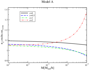
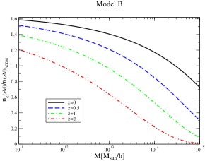
Figure 11: Ratio of comoving number density above mass $M$, computed with the mass function correction Eq. (5.5), $n_{c}(>M)$ to the comoving number density in the $\Lambda$CDM model.

However, let us note once again that the actual number of objects also depends on the comoving volume. Therefore the behaviour observed in Fig. 11 can be modified, especially at high $z$. In order to verify what is the observable effect, we finally compute the total number of clusters above mass $M$ and redshift $z$:

$$N\left(>z,>M\right)=\int_{z}^{\infty}dz^{\prime}\frac{dV^{2}}{dz^{\prime}d\Omega}\int_{M}^{\infty}dM^{\prime}\frac{dn}{dM^{\prime}}\,.$$ (5.6)

In Fig. 12 we show the total number of halos above mass $M$ and $z=1$ (left panel) and $z=2$ (right panel) for $\Lambda$CDM, Model A and Model B. The values for Model A and Model B are computed using the corrected mass function for the perturbative contribution only. For $z>1$ the EDE models present fewer objects than $\Lambda$CDM. The same is true for $z>2$, however Model A and $\Lambda$CDM are much more similar. Therefore, in these specific examples, we can see that the correction in the mass function due to DE mass is not enough to produce more massive and distant clusters than $\Lambda$CDM. Anyhow the main lesson we should take from these results is that if DE possesses fluctuations, its contribution for the halo mass can substantially change the abundance of massive galaxy clusters. The proper description of this effect is of major importance when testing inhomogeneous DE models with observations of such objects.

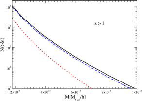
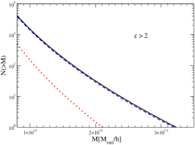
Figure 12: Total number of halos above mass $M$ and $z=1$ (left panel) and $z=2$ (right panel), Eq. (5.6). The solid black lines refers to $\Lambda$CDM model, the blue dashed (red dotted) lines to Model A (Model B), with $c_{\rm eff}=0$ and correct mass function due to the perturbative contribution only.

6 Conclusions

In this paper we have studied the influence of inhomogeneous EDE both in linear and nonlinear stages of structure formation. We have evaluated the matter growth, the ISW effect, the contribution of DE fluctuations for the total mass of the halos, the halo abundance relative to $\Lambda$CDM model and its corrections due the extra DE mass contribution.

We have showed that the presence of large EDE fluctuations, i.e., models with $c_{\rm eff}=0$, have the general property of making DM growth, ISW effect and halo abundance more similar to the predictions of the $\Lambda$CDM model than homogeneous EDE models, those with $c_{\rm eff}=1$. In Model A, the one more similar to $\Lambda$CDM in the background evolution, the differences in $f=d\ln D/d\ln a$ against $\Lambda$CDM predictions are below $5\%$ level, and the impact of DE fluctuations is even smaller. Eventually surveys like Euclid, which can provide data on $f$ with $1\%$ precision [47], will be able to distinguish between homogeneous and inhomogeneous EDE models.

The analysis of the number density of halos initially showed that all EDE models provide fewer density of massive clusters, independently of the redshift considered. For models with nearly smooth EDE this conclusion remains valid. However, for inhomogeneous EDE models, once we account for the extra halo mass associated with DE fluctuations, which we showed that can be of the order of $10\%$, and make the corresponding correction in the mass function, this situation may change. We saw that, at high redshifts, the corrected number density can be larger than in $\Lambda$CDM. This was observed for our Model A with $c_{\rm eff}=0$ at $z=2$. However, after computing the total number of halos, the impact of this correction is supplanted by the effect of the smaller comoving volume of EDE models and $\Lambda$CDM still presents more massive objects.

It is important to stress that, in principle, the magnitude of DE fluctuations that we found and the corresponding impact on observables that we have studied is specific of EDE models. If DE has non-negligible energy density at intermediate and high redshifts the equation-of-state parameter $w$ is close to $0$, which, according with Eq. (3.31), enhances the magnitude of DE fluctuations. However we also showed that inhomogeneous EDE models actually make predictions more similar to $\Lambda$CDM than their homogeneous counterparts. Therefore we conclude that if the accelerated expansion is caused by an inhomogeneous EDE model it will be challenging to distinguish it from the Cosmological Constant.

References

- [1] R. Amanullah et. al., Spectra and light curves of six type ia supernovae at and the union2 compilation, Astrophys. J. 716 (2010) 712–738, [arXiv:1004.1711].
- [2] G. Hinshaw, D. Larson, E. Komatsu, D. Spergel, C. Bennett, et. al., Nine-year wilkinson microwave anisotropy probe (wmap) observations: Cosmological parameter results, arXiv:1212.5226.
- [3] J. L. Sievers, R. A. Hlozek, M. R. Nolta, V. Acquaviva, G. E. Addison, et. al., The atacama cosmology telescope: Cosmological parameters from three seasons of data, arXiv:1301.0824.
- [4] B. A. Reid et. al., Cosmological constraints from the clustering of the sloan digital sky survey dr7 luminous red galaxies, Mon. Not. Roy. Astron. Soc. 404 (2010) 60–85, [arXiv:0907.1659].
- [5] C. Blake, S. Brough, M. Colless, C. Contreras, W. Couch, et. al., The wigglez dark energy survey: the growth rate of cosmic structure since redshift z=0.9, Mon.Not.Roy.Astron.Soc. 415 (2011) 2876, [arXiv:1104.2948].
- [6] S. Weinberg, The cosmological constant problem, Rev.Mod.Phys. 61 (1989) 1–23.
- [7] V. Sahni and A. A. Starobinsky, The case for a positive cosmological lambda term, Int.J.Mod.Phys. D9 (2000) 373–444, [astro-ph/9904398].
- [8] I. Zlatev, L.-M. Wang, and P. J. Steinhardt, Quintessence, cosmic coincidence, and the cosmological constant, Phys. Rev. Lett. 82 (1999) 896–899, [astro-ph/9807002].
- [9] P. J. E. Peebles and B. Ratra, Cosmology with a time variable cosmological ’constant’, Astrophys. J. 325 (1988) L17.
- [10] B. Ratra and P. J. E. Peebles, Cosmological consequences of a rolling homogeneous scalar field, Phys. Rev. D37 (1988) 3406.
- [11] C. Wetterich, Cosmology and the fate of dilatation symmetry, Nucl. Phys. B302 (1988) 668.
- [12] P. J. Steinhardt, L.-M. Wang, and I. Zlatev, Cosmological tracking solutions, Phys. Rev. D59 (1999) 123504, [astro-ph/9812313].
- [13] M. Doran and G. Robbers, Early dark energy cosmologies, JCAP 0606 (2006) 026, [astro-ph/0601544].
- [14] M. Bartelmann, M. Doran, and C. Wetterich, Non-linear structure formation in cosmologies with early dark energy, Astron. Astrophys. 454 (2006) 27–36, [astro-ph/0507257].
- [15] M. J. Francis, G. F. Lewis, and E. V. Linder, Can early dark energy be detected in non-linear structure?, Mon. Not. Roy. Astron. Soc. 394 (2008) 605–614, [arXiv:0808.2840].
- [16] E. Calabrese, D. Huterer, E. V. Linder, A. Melchiorri, and L. Pagano, Limits on dark radiation, early dark energy, and relativistic degrees of freedom, Phys.Rev. D83 (2011) 123504, [arXiv:1103.4132].
- [17] C. L. Reichardt, R. de Putter, O. Zahn, and Z. Hou, New limits on early dark energy from the south pole telescope, Astrophys. J. 749 (2012) L9, [arXiv:1110.5328].
- [18] W. Hu, Structure formation with generalized dark matter, Astrophys. J. 506 (1998) 485–494, [astro-ph/9801234].
- [19] R. R. Caldwell, R. Dave, and P. J. Steinhardt, Cosmological imprint of an energy component with general equation-of-state, Phys. Rev. Lett. 80 (1998) 1582–1585, [astro-ph/9708069].
- [20] C.-G. Park, J.-c. Hwang, J.-h. Lee, and H. Noh, Roles of dark energy perturbations in the dynamical dark energy models: Can we ignore them?, Phys. Rev. Lett. 103 (2009) 151303, [arXiv:0904.4007].
- [21] A. J. Christopherson, Gauge conditions in combined dark energy and dark matter systems, Phys.Rev. D82 (2010) 083515, [arXiv:1008.0811].
- [22] T. Chiba, T. Okabe, and M. Yamaguchi, Kinetically driven quintessence, Phys.Rev. D62 (2000) 023511, [astro-ph/9912463].
- [23] C. Armendariz-Picon, V. F. Mukhanov, and P. J. Steinhardt, Essentials of k essence, Phys.Rev. D63 (2001) 103510, [astro-ph/0006373].
- [24] L. P. Chimento and R. Lazkoz, Atypical k-essence cosmologies, Phys.Rev. D71 (2005) 023505, [astro-ph/0404494].
- [25] P. Creminelli, G. D’Amico, J. Norena, and F. Vernizzi, The effective theory of quintessence: the w¡-1 side unveiled, JCAP 0902 (2009) 018, [arXiv:0811.0827].
- [26] J. K. Erickson, R. Caldwell, P. J. Steinhardt, C. Armendariz-Picon, and V. F. Mukhanov, Measuring the speed of sound of quintessence, Phys.Rev.Lett. 88 (2002) 121301, [astro-ph/0112438].
- [27] R. Bean and O. Dore, Probing dark energy perturbations: the dark energy equation of state and speed of sound as measured by wmap, Phys. Rev. D69 (2004) 083503, [astro-ph/0307100].
- [28] W. Hu and R. Scranton, Measuring dark energy clustering with cmb-galaxy correlations, Phys.Rev. D70 (2004) 123002, [astro-ph/0408456].
- [29] D. Sapone, M. Kunz, and M. Kunz, Fingerprinting dark energy, Phys. Rev. D80 (2009) 083519, [arXiv:0909.0007].
- [30] R. de Putter, D. Huterer, and E. V. Linder, Measuring the speed of dark: Detecting dark energy perturbations, Phys.Rev. D81 (2010) 103513, [arXiv:1002.1311].
- [31] S. Basilakos, J. C. Bueno Sanchez, and L. Perivolaropoulos, The spherical collapse model and cluster formation beyond the cosmology: Indications for a clustered dark energy?, Phys. Rev. D80 (2009) 043530, [arXiv:0908.1333].
- [32] M. Grossi and V. Springel, The impact of early dark energy on non-linear structure formation, Mon.Not.Roy.Astron.Soc. 394 (2009) 1559–1574, [arXiv:0809.3404].
- [33] J.-Q. Xia and M. Viel, Early dark energy at high redshifts: Status and perspectives, JCAP 0904 (2009) 002, [arXiv:0901.0605].
- [34] F. Pace, J.-C. Waizmann, and M. Bartelmann, Spherical collapse model in dark-energy cosmologies, Mon. Not. Roy. Astron. Soc. 406 (2010) 1865–1874, [arXiv:1005.0233].
- [35] U. Alam, Constraining perturbative early dark energy with current observations, Astrophys.J. 714 (2010) 1460–1469, [arXiv:1003.1259].
- [36] U. Alam, Z. Lukic, and S. Bhattacharya, Galaxy clusters as a probe of early dark energy, Astrophys.J. 727 (2011) 87, [arXiv:1004.0437].
- [37] F. Wang, Current constraints on early dark energy and growth index using latest observations, Astron.Astrophys. 543 (2012) A91.
- [38] P. S. Corasaniti and E. J. Copeland, A model independent approach to the dark energy equation of state, Phys. Rev. D67 (2003) 063521, [astro-ph/0205544].
- [39] C.-P. Ma and E. Bertschinger, Cosmological perturbation theory in the synchronous and conformal newtonian gauges, Astrophys. J. 455 (1995) 7–25, [astro-ph/9506072].
- [40] M. Li, Y. Cai, H. Li, R. Brandenberger, and X. Zhang, Dark energy perturbations revisited, Phys. Lett. B702 (2011) 5–11, [arXiv:1008.1684].
- [41] G. Ballesteros and J. Lesgourgues, Dark energy with non-adiabatic sound speed: initial conditions and detectability, JCAP 1010 (2010) 014, [arXiv:1004.5509].
- [42] R. U. H. Ansari and S. Unnikrishnan, Perturbations in dark energy models with evolving speed of sound, arXiv:1104.4609.
- [43] T. Basse, O. E. Bjaelde, and Y. Y. Y. Wong, Spherical collapse of dark energy with an arbitrary sound speed, JCAP 1110 (2011) 038, [arXiv:1009.0010].
- [44] T. Basse, O. E. Bjaelde, S. Hannestad, and Y. Y. Y. Wong, Confronting the sound speed of dark energy with future cluster surveys, arXiv:1205.0548.
- [45] L. R. Abramo, R. C. Batista, L. Liberato, and R. Rosenfeld, Physical approximations for the nonlinear evolution of perturbations in inhomogeneous dark energy scenarios, Phys. Rev. D79 (2009) 023516, [arXiv:0806.3461].
- [46] P. Creminelli, G. D’Amico, J. Norena, L. Senatore, and F. Vernizzi, Spherical collapse in quintessence models with zero speed of sound, JCAP 1003 (2010) 027, [arXiv:0911.2701].
- [47] Euclid Theory Working Group Collaboration, L. Amendola et. al., Cosmology and fundamental physics with the euclid satellite, arXiv:1206.1225.
- [48] R. K. Sachs and A. M. Wolfe, Perturbations of a cosmological model and angular variations of the microwave background, Astrophys. J. 147 (1967) 73–90.
- [49] T. Giannantonio, R. Crittenden, R. Nichol, and A. J. Ross, The significance of the integrated sachs-wolfe effect revisited, Mon.Not.Roy.Astron.Soc. 426 (2012) 2581–2599, [arXiv:1209.2125].
- [50] D. F. Mota and C. van de Bruck, On the spherical collapse model in dark energy cosmologies, Astron. Astrophys. 421 (2004) 71–81, [astro-ph/0401504].
- [51] N. J. Nunes and D. F. Mota, Structure formation in inhomogeneous dark energy models, Mon. Not. Roy. Astron. Soc. 368 (2006) 751–758, [astro-ph/0409481].
- [52] L. R. Abramo, R. C. Batista, L. Liberato, and R. Rosenfeld, Structure formation in the presence of dark energy perturbations, JCAP 0711 (2007) 012, [0707.2882].
- [53] L. R. Abramo, R. C. Batista, and R. Rosenfeld, The signature of dark energy perturbations in galaxy cluster surveys, JCAP 0907 (2009) 040, [arXiv:0902.3226].
- [54] T. G. Brainerd, R. J. Scherrer, and J. V. Villumsen, Linear evolution of the gravitational potential: A new approximation for the nonlinear evolution of large scale structure, Astrophys. J. 418 (1993) 570.
- [55] J. S. Bagla and T. Padmanabhan, Nonlinear evolution of density perturbations using approximate constancy of gravitational potential, Mon. Not. Roy. Astron. Soc. 266 (1994) 227, [gr-qc/9304021].
- [56] J. E. Gunn and J. R. I. Gott, On the infall of matter into cluster of galaxies and some effects on their evolution, Astrophys. J. 176 (1972) 1–19.
- [57] T. Padmanabhan, Structure Formation in the Universe. Cambridge University Press, 1993.
- [58] W. J. Percival, Cosmological structure formation in a homogeneous dark energy background, Astron. Astrophys. 443 (2005) 819, [astro-ph/0508156].
- [59] M. J. Francis, G. F. Lewis, and E. V. Linder, Halo mass functions in early dark energy cosmologies, Mon.Not.Roy.Astron.Soc.Lett. 393 (2008) L31–L35, [arXiv:0810.0039].
- [60] S. Lee and K.-W. Ng, Spherical collapse model with non-clustering dark energy, JCAP 1010 (2010) 028, [arXiv:0910.0126].
- [61] S. Meyer, F. Pace, and M. Bartelmann, Relativistic virialization in the spherical collapse model for einstein-de sitter and cdm cosmologies, Phys.Rev. D86 (2012) 103002, [arXiv:1206.0618].
- [62] O. Lahav, P. B. Lilje, J. R. Primack, and M. J. Rees, Dynamical effects of the cosmological constant, Mon. Not. Roy. Astron. Soc. 251 (1991) 128–136.
- [63] I. Maor and O. Lahav, On virialization with dark energy, JCAP 0507 (2005) 003, [astro-ph/0505308].
- [64] A. Chernin, P. Teerikorpi, M. Valtonen, G. Byrd, V. Dolgachev, et. al., Dark energy and the mass of the local group, arXiv:0902.3871.
- [65] R. K. Sheth and G. Tormen, Large-scale bias and the peak background split, MNRAS 308 (Sept., 1999) 119–126, [astro-ph/].
- [66] R. K. Sheth and G. Tormen, An excursion set model of hierarchical clustering: ellipsoidal collapse and the moving barrier, MNRAS 329 (Jan., 2002) 61–75, [astro-ph/].
- [67] R. K. Sheth, H. J. Mo, and G. Tormen, Ellipsoidal collapse and an improved model for the number and spatial distribution of dark matter haloes, MNRAS 323 (May, 2001) 1–12, [astro-ph/].
- [68] J. M. Bardeen, J. R. Bond, N. Kaiser, and A. S. Szalay, The statistics of peaks of gaussian random fields, Astrophys. J. 304 (1986) 15–61.
- [69] WMAP Collaboration, E. Komatsu et. al., Seven-year wilkinson microwave anisotropy probe (wmap) observations: Cosmological interpretation, Astrophys. J. Suppl. 192 (2011) 18, [arXiv:1001.4538].
- [70] D. Larson, J. Dunkley, G. Hinshaw, E. Komatsu, M. R. Nolta, C. L. Bennett, B. Gold, M. Halpern, R. S. Hill, and et al., Seven-year wilkinson microwave anisotropy probe (wmap) observations: Power spectra and wmap-derived parameters, ApJS 192 (Feb., 2011) 16–+, [arXiv:1001.4635].
- [71] C. G. Lacey and S. Cole, Merger rates in hierarchical models of galaxy formation, Mon.Not.Roy.Astron.Soc. 262 (1993) 627–649.
- [72] M. J. Mortonson, W. Hu, and D. Huterer, Simultaneous falsification of cdm and quintessence with massive, distant clusters, Phys.Rev. D83 (2011) 023015, [arXiv:1011.0004].