Local Gaussian process approximation for large computer experiments

Abstract

We provide a new approach to approximate emulation of large computer experiments. By focusing expressly on desirable properties of the predictive equations, we derive a family of local sequential design schemes that dynamically define the support of a Gaussian process predictor based on a local subset of the data. We further derive expressions for fast sequential updating of all needed quantities as the local designs are built-up iteratively. Then we show how independent application of our local design strategy across the elements of a vast predictive grid facilitates a trivially parallel implementation. The end result is a global predictor able to take advantage of modern multicore architectures, providing a nonstationary modeling feature as a bonus. We demonstrate our method on two examples utilizing designs with thousands of data points, and compare to the method of compactly supported covariances.

Key words: sequential design, sequential updating, active learning, surrogate model, emulator, compactly supported covariance, local kriging neighborhoods

1 Introduction

The Gaussian process (GP) is a popular choice for emulating computer experiments (Santner et al.,, 2003). As priors for nonparametric regression, they are unparalleled; they are rarely beaten in out-of-sample predictive tests, have appropriate coverage, and have an attractive ability to accomplish these feats while interpolating the response if so desired. That said, GPs do have disadvantages, for example: (1) computation (for inference and prediction) scales poorly as data sets get large; and (2) the best results require an assumption of stationarity in the data-generating mechanism, which may not be appropriate. The second issue is usually coupled with the first. Emulators relaxing stationarity exist, but often at further computational expense. Examples include learning nonlinear mappings to a space where stationarity reigns (e.g. Schmidt and O’Hagan,, 2003, and references therein), and process convolution approaches that allow the kernels to vary smoothly in parameterization as an unknown function of their spatial location (e.g., Paciorek and Schervish,, 2006, and therein).

Several works in recent literature have made inroads in reducing the computational burden for stationary models, usually by making some kind of approximation. Examples include searching for a reduced set of “pseudo-inputs” (Snelson and Ghahramani,, 2006), building up estimators iteratively (e.g., Haaland and Qian,, 2011; Gramacy and Polson,, 2011), fixed rank kriging (Cressie and Johannesson,, 2008), compactly supported (sparse) covariance (CSC) (Kaufman et al.,, 2012). Our contribution has aspects in common with all of these approaches and several others by association. It is reminiscent of ad hoc methods based on local kriging neighborhoods (e.g., Cressie,, 1991, pp. 131–134). What we propose is more modern, scalable, ideally suited to multicore computing, and tailored to computer experiments. It draws in part on recent findings for approximate likelihoods in spatial data (e.g., Stein et al.,, 2004), and active learning techniques (e.g., Cohn,, 1996).

We start by focusing on the prediction problem, locally, at an input $x$. In computer model emulation this is the primary problem of interest. We recognize, as many authors have before us, that data points far from $x$ have vanishingly small influence on the predictive distribution (assuming the usual choices of covariance). Thus, even though a large covariance matrix may have been calculated and inverted at great computational expense, not many of its rows/columns contribute substantively to the linear predictor. We focus on finding those data points (relative to $x$), and corresponding rows/cols, without considering the full matrices. In particular, we illustrate how a sensible objective criterion reduces to a key component of an active learning heuristic that has found recent application in the design of computer experiments literature (see, e.g., Gramacy and Lee,, 2009).

Our localized sub-designs differ from a local nearest neighbor (NN) approach, and yield more accurate predictions for a fixed local design size. This echoes a result by Stein et al., (2004) who observe that NNs may not be ideal for learning correlation parameters. We extend that to obtaining predictions, although we recognize that a modern take on NN can represent an attractive option, computationally, in many contexts. Our methods are applicable with any covariance family that can be differentiated analytically. However, we deliberately choose a very naïve one and nonetheless compare favorably to others having more thoughtful choices (e.g., Kaufman et al.,, 2012). The explanation is that we leverage a globally nonstationary effect that compensates for an overly smooth/simplistic local structure.

There are strong parallels between our suggested approach and CSC, although there are two key distinctions. The first is that our method is purely local, whereas a substantial innovation in CSC is to take a local–global hybrid approach. CSC estimates a global mean structure via a polynomial basis in order to “soak up” large scale variabilities in the spatial field. Second, we are not applying any kind of tapering of influence in learning that local structure. Tapering is a smooth operation which would retain most of the features, e.g., stationary, of an un-tapered analog. However our approach is discrete and therefore could not retain stationarity or smoothness. Our main advantage is that accuracy can be explicitly linked to a computational budget—we know exactly how “sparse” our matrices will be before running the code, and we can monitor convergence to the (intractable) full-data counterparts. Also, since we focus on particular locations $x$, independent of others, our method is highly parallelizable. Local inference for many $x$’s can proceed without communication between nodes, meaning that OpenMP pragmas can yield nearly-linear speedups.

The remainder of the paper is outlined as follows. In Section 2 we review GP predictive modeling, inference and prediction. In Section 3 we derive a criteria for greedily building local designs, expressions for the efficient updating of all required quantities, and argue that a simpler heuristic from the active learning literature may prove to be even more efficient. Section 4 treats global prediction problem, for many $x$, and discusses global inference for the correlation structure. Finally, all of the elements are brought together in Section 5 for empirical illustrations and comparisons to CSC. We conclude with a discussion in Section 6. An implementation of our methods can be found in the laGP (Gramacy,, 2013) for R.

2 Gaussian process predictive modeling

A GP prior for functions $Y\!:\mathbb{R}^{p}\rightarrow\mathbb{R}$, where any finite collection of outputs are jointly Gaussian, is defined by its mean $\mu(x)=\mathbb{E}\{Y(x)\}$ and covariance $C(x,x^{\prime})=\mathbb{E}\{[Y(x)-\mu(x)][Y(x^{\prime})-\mu(x^{\prime})]^{\top}\}$. A common simplifying assumption in the computer modeling literature is to take the mean to be zero, and this is the convention we will follow. Typically, one separates out the variance $\tau^{2}$ in $C(x,x^{\prime})$ and works with correlations $K(x,x^{\prime})=\tau^{-2}C(x,x^{\prime})$ based on Euclidean distance and a small number of unknown parameters. In this paper we focus on the isotropic Gaussian correlation $K_{\theta,\eta}(x,x^{\prime})=\exp\{-||x-x^{\prime}||^{2}/\theta\}+\eta\delta_{x,x^{\prime}}$ where $\theta$ is called the lengthscale parameter, and $\eta$ the nugget.

In what follows we hold $\eta$ at a pre-determined small value in order to obtain a near-interpolative surface which is appropriate when the computer model is deterministic. It is important to note that our main results do not heavily depend on of the choice of correlation function so long as derivatives (with respect to $\theta$) are available. The isotropic, one-parameter $(\theta)$ family simplifies the exposition. However the derivations of our main results [Section SM§2] assume a separable family. The laGP package facilitates estimating $\eta$ if desired.

Although technically a prior over functions, the regression perspective recommends a likelihood interpretation. Using data $D=(X,Y)$, where $X$ is a $N\times p$ design matrix, the $N\times 1$ response vector $Y$ has a multivariate normal (MVN) likelihood with mean zero and covariance $\Sigma(X)=\tau^{2}K$, where $K$ is an $N\times N$ matrix with $(ij)^{\mathrm{th}}$ entry $K(x_{i},x_{j})$. Conditional on $K$, the MLE of $\tau^{2}$ is available analytically. Profile likelihoods may then be used to infer other unknown parameters (e.g., $\theta$).

Empirical Bayes (Berger et al.,, 2001) has gained in popularity recently. In this approach one specifies a reference prior, $\pi(\tau^{2})\propto\tau^{-2}$. Having an MVN likelihood, and prior algebraically equivalent to IG$(0,0)$, makes integrating over $\tau^{2}$ analytic. We obtain

$$p(Y|K)=\frac{\Gamma[N/2]}{(2\pi)^{N/2}|K|^{1/2}}\times\left(\frac{\psi}{2}\right)^{\!-\frac{N}{2}},\;\;\;\;\;\mbox{where}\;\;\;\psi=Y^{\top}K^{-1}Y.$$ (1)

Newton-like methods for estimating $\theta$ work well when leveraging derivative information for the log likelihood [see SM§2], and when the likelihood surface is not multi-modal.

The marginalized predictive equations for GP regression, i.e., for $Y(x)$ given on data $D$ and covariance $K(\cdot,\cdot)$, are Student-$t$ with degrees of freedom $N$,

mean $$\mu(x|D,K) =k^{\top}(x)K^{-1}Y,$$ (2)

and scale $$\sigma^{2}(x|D,K) =\frac{\psi[K(x,x)-k^{\top}(x)K^{-1}k(x)]}{N},$$ (3)

where $k^{\top}(x)$ is the $N$-vector whose $i^{\mbox{\tiny th}}$ component is $K(x,x_{i})$. Using properties of the Student-$t$, the variance of $Y(x)$ is $V(x)\equiv\mathbb{V}\mathrm{ar}[Y(x)|D]=\sigma^{2}(x|D,K)\times N/(N-2)$.

3 Localized approximate emulation

If obtaining fast approximate prediction at $x$ is the goal, then a first stab may be to use a small sub-design of $X$ locations closest to $x$. I.e., choose the $n$-nearest neighbor (NN) sub-design $X_{n}(x)\subseteq X$ and apply the predictive equations (2–3) with $D_{n}(x)=(X_{n},Y_{n})$ where $n$ is chosen as large as computational constraints allow. This is a sensible approach. It is clearly an approximation: as $n\rightarrow N$, $Y(x)|D_{n}$ converges to $Y(x)|D$ trivially. Moreover, since the predictive equations are valid for any design, interpreting the accuracy of the approximation involves the same quantities as those obtained from an analysis based the on full design. Clearly, when $n\ll N$, the variance $V(x)|D_{n}$ can be much larger than $V(x)|D$. However, if $N$ is so big as to preclude obtaining any predictor at all, within reasonable computational constraints, obtaining one with marginally inflated uncertainty is better than nothing.

Though simple, one naturally wonders if it is optimal for fixed $n$. It is not: Vecchia, (1988) observed that the best sub-design for prediction depends $\theta$, and is usually not the NN design. In fact, NN is uniformly suboptimal under certain conditions (Stein et al.,, 2004). Still, finding the best design for $n>1$ is hard, involving a high-dimensional non-convex optimization. Joint inference with $\theta$ can compound that expense. Simple NN seems pragmatic by comparison, but we show how to do better without much extra effort.

Our main idea, which is akin to forward stepwise variable selection in regression, is as follows. For a particular predictive location $x$, we search for a sub-design $X_{n}(x)$, with accompanying responses $Y_{n}(x)$, together comprising data $D_{n}(x)$, by making a sequence of greedy decisions $D_{j+1}(x)=D_{j}(x)\cup(x_{j+1},y(x_{j+1}))$, $j=n_{0},\dots,n$. Each choice of $x_{j+1}$ depends on the previous choices saved in $D_{j}(x)$ by searching over a criterion. Evaluating the criterion, and updating the quantities required for the next iteration, must not exceed $O(j^{2})$ so that the total scheme remains $O(n^{3})$, like NN. We start with a very small $D_{n_{0}}(x)$ comprised of $n_{0}$ NNs, which is easy to motivate in light of results shown in Section 3.4.

3.1 Greedy search to minimize mean-squared predictive error

Given $x$ and $D_{j}(x)$, we search for $x_{j+1}$ by considering its impact on the variance of $Y(x)$, taking into account uncertainty in $\theta$, through an empirical Bayes mean-square prediction error (MSPE) criterion: $J(x_{j+1},x)=\mathbb{E}\{[Y(x)-\mu_{j+1}(x;\hat{\theta}_{j+1})]^{2}|D_{j}(x)\}$, which should be minimized. The predictive mean $\mu_{j+1}(x;\hat{\theta}_{j+1})$ follows (2), although we embellish notation here to explicitly indicate dependence on $x_{j+1}$ and the future $y_{j+1}$. This mean represents the hypothetical prediction of $Y(x)$ arising after choosing $x_{j+1}$, observing $y_{j+1}$, and calculating the MLE $\hat{\theta}_{j+1}$ based on the resulting $D_{j+1}(x)$. Where convenient we drop the $x$ argument in the local design, $D_{j}\equiv D_{j}(x)$. Also note that $\hat{\theta}_{j}\equiv\hat{\theta}_{j}(x)$ since it depends on $D_{j}(x)$.

In Section SM§2 we derive the approximation

$$J(x_{j+1},x)\approx V_{j}(x|x_{j+1};\hat{\theta}_{j})+\left(\frac{\partial\mu_{j}(x;\theta)}{\partial\theta}\Big{|}_{\theta=\hat{\theta}_{j}}\right)^{2}/\mathcal{G}_{j+1}(\hat{\theta}_{j}).$$ (4)

The terms in (4) are explained below in turn.

• $V_{j}(x|x_{j+1};\theta)$ is the new variance after adding $x_{j+1}$ into $D_{j}$, treating $\theta$ as known.

  $$V_{j}(x|x_{j+1};\theta) =\frac{\psi_{j}}{j-2}v_{j+1}(x;\theta),$$

  $$\mbox{where }\;\;\;v_{j+1}(x;\theta) =\left[K_{j+1}(x,x)-k_{j+1}^{\top}(x)K_{j+1}^{-1}k_{j+1}(x)\right]$$ (5)

  captures $x_{j+1}$’s contribution to the reduction in variance by placing its correlations to $X_{j}$ in the $j+1^{\mathrm{st}}$ row/col of $K_{j+1}$. The correlation between $x$ and $X_{j+1}(x)\equiv(X_{j}(x),x_{j+1})$ comes in through the $j+1^{\mathrm{st}}$ entry of $k_{j+1}$, the rest being $k_{j}$.

• $\frac{\partial\mu_{j}(x;\theta)}{\partial\theta}$ is the derivative of the predictive mean (2) at $x$, given $D_{j}$, with respect to $\theta$.

  $$\frac{\partial\mu_{j}(x;\theta)}{\partial\theta}=[\dot{k}_{j}(x)-\dot{\mathcal{K}}_{j}k_{j}(x)]^{\top}K_{j}^{-1}Y_{j},$$ (6)

  where $\dot{\mathcal{K}}_{j}=\dot{K}_{j}K_{j}^{-1}$ and $\dot{k}_{j}(x)$ is the $j$-length column vector of derivatives of the correlation function $K(x,x_{k})$, $k=1,\dots,j$, with respect to $\theta$.

• $\mathcal{G}_{j+1}(\theta)$ is the expected Fisher information comprised of the information from $D_{j}$ plus the expected component from the future $y_{j+1}$ at $x_{j+1}$:

  $$\mathcal{G}_{j+1}(\theta) =F_{j}(\theta)+\mathbb{E}\left\{-\frac{\partial^{2}\ell_{j}(y_{j+1};\theta)}{\partial\theta^{2}}\Big{|}D_{j};\theta\right\}$$ (7)

  $$\approx F_{j}(\theta)+\frac{1}{2V_{j}(x_{j+1};\theta)^{2}}\times\left(\frac{\partial V_{j}(x_{j+1};\theta)}{\partial\theta}\right)^{2}+\frac{1}{V_{j}(x_{j+1};\theta)}\left(\frac{\partial\mu_{j}(x_{j+1};\theta)}{\partial\theta}\right)^{2},$$

  where $F_{j}(\theta)=-\ell^{\prime\prime}(Y_{j};\theta)$ from (SM.4), $V_{j}(x_{j+1};\theta)\equiv V(x_{j+1}|D_{j};\theta)$ following (3), and

  $$\frac{\partial V_{j}(x;\theta)}{\partial\theta} =\frac{Y_{j}^{\top}K_{j}^{-1}\dot{\mathcal{K}}_{j}Y_{j}}{j-2}\left(K(x,x)-k_{j}^{\top}(x)\tilde{k}_{j}(x)\right)$$

  $$\;\;-\!\frac{\psi_{j}}{j-2}\left[\dot{k}_{j}^{\top}(x)\tilde{k}_{j}(x)+\tilde{k}_{j}(x)^{\top}(\dot{k}_{j}(x)\!-\!\dot{\mathcal{K}}_{j}k_{j}(x))\right]\!,\mbox{ where }\tilde{k}_{j}(x)=K_{j}^{-1}k_{j}(x).$$

The approximation in (4) is three-fold: (a) the partial derivative of $\mu_{j+1}$ is approximated by that of $\mu_{j}$; (b) the Student-$t$ predictive equations are approximated by moment-matched Gaussian ones (7); and (c) the future $\hat{\theta}_{j+1}$ is replaced by the current estimate $\hat{\theta}_{j}$ based on the data $D_{j}$ obtained so far. All are required since averaging over future expected $y_{j+1}$ is analytically intractable. Even though a $y_{j+1}$ is technically available in our context, we deliberately do not condition on this value, which would result in the undesirable avoidance of selecting an $x_{j+1}$ whose $y_{j+1}$ is at odds with $D_{j}$. [More discussion in SM§2.]

Observe that when the Fisher information is large, the MSPE (4) is dominated by the reduced variance for $x_{j+1}$, the first term. We return to this special case in Section 3.3. For smaller $j$ the extra term gives preference to choosing an $x_{j+1}$ that is expected to improve estimates of $\theta$ nearby to $x$. Considering that a sensible non-local design strategy is to maximize (the determinant of) the Fisher information, the MSPE is thus making a local adjustment by (a) weighting the Fisher information by the rate of change of the predictive mean near $x$ and (b) balancing that with the aim of reducing local predictive variance. The appropriate balance is automatically dictated by the definition of $J(x_{j+1},x)$, which considers the effect of uncertainty in $\theta$ on the predictive uncertainty in $Y(x)$. Aspect (a) is suggestive of potential benefit in estimating a localized, i.e., nonstationary, spatial field.

3.2 Fast updates

All required quantities can be updated quickly, from iteration $j$ to $j+1$, in $O(j^{2})$ time so that $n$ applications are in $O(n^{3})$. This is possible since $K_{j+1}^{-1}$ can be obtained efficiently from $K_{j}^{-1}$, both conditional on the same parameter $\theta$, via the partition inverse equations [see SM§1]. We use them in several applications. For example,

$$v_{j}(x ;\theta)-v_{j+1}(x;\theta),\quad\mbox{(dropping $\theta$ below for compactness)}$$ (8)

$$=k_{j}^{\top}(x)G_{j}(x_{j+1})v_{j}(x_{j+1})k_{j}(x)+2k_{j}^{\top}(x)g_{j}(x_{j+1})K(x_{j+1},x)+K(x_{j+1},x)^{2}/v_{j}(x_{j+1}),$$

where $G_{j}(x^{\prime})\equiv g_{j}(x^{\prime})g_{j}^{\top}(x^{\prime})$, and $g_{j}(x^{\prime})=K_{j}^{-1}k_{j}(x^{\prime})/v_{j}(x^{\prime})$. Each product above requires most $O(j^{2})$ time. Adding a row and column $k_{j}(x_{j+1})$ to $K_{j}$ yields $K_{j+1}$ in $O(j)$ extra time. The log marginal likelihood requires $\log|K_{j}|$, which may similarly be updated as

$$\log|K_{j+1}| =\log|K_{j}|+\log(K(x_{j+1},x_{j+1})+g_{j}^{\top}(x_{j+1})k_{j}(x_{j+1})v_{j}(x_{j+1}))$$

$$=\log|K_{j}|+\log(v_{j}(x_{j+1})).$$

in $O(j)$ time. Fast updates are available for key aspects of the predictive equations (2–3):

$$K_{j+1}^{-1}Y_{j+1} =\begin{pmatrix}K_{j}^{-1}Y_{j}+g_{j}(x_{j+1})(h_{j}(x_{j+1})v_{j}(x_{j+1})+y_{j+1})\\ h_{j}(x_{j+1})+y_{j+1}/v_{j}(x_{j+1})\end{pmatrix}$$

$$\mbox{and }\;\;\psi_{j+1} =\psi_{j}+h_{j}(x_{j+1})^{2}v_{j}(x_{j+1})+2y_{j+1}h_{j}(x_{j+1})+y_{j+1}^{2}/v_{j}(x_{j+1}),$$ (9)

where $h_{j}(x_{j+1})=Y_{j}^{\top}g_{j}(x_{j+1})$. Both updates take time in $O(j)$.

For fast updates of the observed information $F_{j+1}(\theta)$, write the log likelihood as a sum of components from $D_{j}$ and from $(x_{j+1},y_{j+1})$, with the latter denoted by $\ell_{j}(y_{j+1};\theta)$. This suggests the simple recursion $F_{j+1}(\theta)=F_{j}(\theta)+\frac{\partial^{2}\ell_{j}(y_{j+1};\theta)}{\partial\theta^{2}}$. In SM§2 we show that

$$\frac{\partial^{2}\ell_{j}(y_{j+1};\theta)}{\partial\theta^{2}}=-\frac{\ddot{V}_{j}}{2V_{j}}\!+\!\frac{\dot{V}_{j}^{2}}{2V_{j}^{2}}\!-\!\frac{\dot{\mu}_{j}^{2}}{V_{j}}+(y_{j+1}-\mu_{j})\!\left(\frac{\ddot{\mu}_{j}}{V_{j}}-2\frac{\dot{\mu}_{j}\dot{V}_{j}}{V_{j}^{2}}\right)+(y_{j+1}-\mu_{j})^{2}\!\left(\frac{\ddot{V}_{j}}{2V_{j}^{2}}-\frac{\dot{V}_{j}^{2}}{V_{j}^{3}}\right).$$

For compactness we are suppressing arguments to the mean and variance functions, and shorthanding their derivatives. E.g., $V_{j}\equiv V_{j}(x_{j+1};\theta)$ and $\ddot{\mu}_{j}\equiv\frac{\partial^{2}\mu_{j}(x_{j+1};\theta)}{\partial\theta^{2}}$. Expressions for second derivatives of predictive quantities may als be found in SM§2. Observe that the expectation (given $D_{j}$) of the above quantity augments $F_{j}(\theta)$ to complete $\mathcal{G}_{j+1}(\theta)$ in (7).

Updates of all other quantities required for the calculations in Section 3.1 follow trivially. Since they require fixed $\theta$, our greedy scheme is only efficient if MLEs are not recalculated after each sequential design decision, suggesting further approximation is warranted to obtain a thrifty MSPE-based local design. We find that working with a reasonable fixed value of $\theta$ throughout the iterations works well. At the end of the $n$ local design and update steps we can find the MLE $\hat{\theta}_{n}(x)$ by Newton-like methods with analytic derivatives (SM.3–SM.4), incurring an $O(n^{3})$ cost once. More details on local inference are deferred to Section 4.2.

3.3 A special case

When the Fisher information is large, the MSPE (4) reduces to $V_{j}(x|x_{j+1};\theta)$, which is the new variance at $x$ when $x_{j+1}$ is added into the design [Section 3.1]. A similar statistic has been used in the sequential design of computer experiments before, but in a different context: choosing design locations for new computer simulations (e.g., Seo et al.,, 2000; Gramacy and Lee,, 2009). Rather than focus on a single $x$, those works average reductions in variance over the whole input space $\mathcal{X}$: $\Delta V_{j}(x_{j+1};\theta)=\int_{\mathcal{X}}(V_{j}(x;\theta)-V_{j}(x|x_{j+1};\theta))\,dx.$ Part of the integrand does not depend on $x_{j+1}$, and so can be ignored. The other part is proportional to $v_{j+1}(x;\theta)$ in (8). In the special case where $K(\cdot,\cdot)$ yields the identity (Anagnostopoulos and Gramacy,, 2013), or when $\mathcal{X}$ is a finite and discrete set, the integral is also analytic. Otherwise numerical methods are needed, which may add significant computational burden.

Choosing $x_{j+1}$ to maximize $\Delta V_{j}(x_{j+1};\theta)$ is a sensible heuristic since it augments the design with an input-output pair that has the most potential to reduce variance globally. In repeated application, $j=1,\dots,N$, the resulting designs have been shown to approximate maximum information designs (Cohn,, 1996). To credit its originator, subsequent authors have referred to this technique as active learning Cohn (ALC). However, the expensive numerical integration required means that alternative heuristics are usually preferred.

A local design criteria based on the integrand alone—the simplest implementation of which involves maximizing (8)—may therefore be a sensible alternative to MSPE, not just further approximation. It has information theoretic motivation and shortcuts cumbersome derivative calculations. In what follows we overload the terminology a bit and refer to local design based on maximizing (8) as ALC. However, it is important to note that its application in this context is novel. ALC in its original form has never been used to select a local sub-design and, since no integration is needed (numerical or otherwise) the computation is straightforward. In SM§4 we show that this heuristic can be derived by studying partial correlations akin to those used to obtain sequential least squares estimators.

3.4 An illustration

Consider a surface first studied by Gramacy and Lee, (2011b), defined by $f(x_{1},x_{2})=-w(x_{1})w(x_{2})$, where $w(x)=\exp\left(-(x-1)^{2}\right)+\exp\left(-0.8(x+1)^{2}\right)-0.05\sin\left(8(x+0.1)\right)$, generating a data set of $x$-$y$ pairs on dense $201\times 201$ ($=40401$ point) regular grid in $[-2,2]$.

Figure 1: A comparison between ALC (black) and MSPE (green) heuristics at two predictive locations. The numbers plotted indicate the order in which the design sites were chosen.

Figure 1 shows local designs for two input locations, $x$, under MSPE and ALC criteria. Both share the same initial design $D_{n_{0}}$ comprising the closest six NNs to $x$. Although the two heuristics agree on some sites chosen, observe that they are not selected in the same order after iteration nine. The patterns diverge most for further out sites, but their qualitative flavor remains similar. In both cases, the bounding box $[-2,2]^{2}$ impacts local design symmetry.

The full 46 local design iterations take less than a tenth of a second on a modern iMac, although in repeated trials (to remove OS noise) we found that MSPE takes 2-3 times longer. Inverting a $40K\times 40K$ matrix cannot, to our knowledge, be done on a modern desktop primarily due to memory swapping issues. For a point of reference, inverting a $4000\times 4000$ matrix took us about seven seconds using a multithreaded BLAS/Lapack. Memory issues aside we deduce that the alternative full-GP result would have taken days.

Figure 2: Comparing the NN predictor to the greedy approach in 1000 repeated repetitions an LHS of size 10001: 10K train/1 test. Both methods are initialized with an NN design $n_{0}=6$. The left pane shows the actual bias and precision and the right shows the predicted precision (GP predictive standard deviation). Each repetition is shown in light shades; the darker dashed lines are 90% quantiles, and the dark solid line is the average. The open-circles with whiskers at $j=52$ are the 90% quantile and average results from a size 1000 NN design.

Figure 2 illustrates the accuracy of the approximate predictive distribution thus obtained, with comparison to the NN alternative. These results summarize the output of a Monte Carlo experiment repeated 1000 times, whose setup is similar to that above with the following exception. In each repetition we generated a Latin Hypercube sample (LHS) of size 10001, and treated the first 10K as training $(X,Y)$ and the last one as our testing $(x,y)$. We then obtained the predictive equations under NN and greedy/MSPE local designs (to $x$) of size $n=50$, where both share a starting NN design $D_{n_{0}}$ of size $n_{0}=6$. Each lightly-shaded line in the plot represents one Monte Carlo iteration. The dark-dashed lines outline point-wise 90% intervals, and the dark-solid lines show the point-wise averages. The open circles and whiskers at 52 on the $j$-axis provide an approximate benchmark, based on a NN local design of size 1000, for the best possible results.

The left pane shows the bias, defined as the predictive mean $\mu_{n}(x)$ minus the true $y$-value. Notice how, relative to the greedy/MSPE method, the NN approach is slow to converge to the true value and is consistently biased low after the initial design. Both start biased-low, which we attribute to $0$-mean reversion typical (for GPs) in areas of the input space sparsely covered by the design. The right pane shows the predicted standard deviation over design iterations. Notice that the NN standard deviations are consistently lower than those from the greedy/MSPE method. So the NN method is both biased-low and more confident than its comparator. At $j=n=50$ both methods obtain a predictive mean close to the truth, with lower variability for the greedy/MSPE method. Moreover, both adequately acknowledge uncertainty inherent in the approximation obtained using a much smaller local design compared to one obtained with orders of magnitude larger designs. In the SM§3 we show that an added benefit of the greedy approach is that the condition numbers of $K_{j}$ are lower than those obtained from NN.

4 Global emulation on a dense design

The simplest way to extend the analysis to cover a dense design of predictive locations $x\in\mathcal{X}$ is to serialize: loop over each $x$ collecting approximate predictive equations, each in $O(n^{3})$ time. For $T=|\mathcal{X}|$ the total computational time is in $O(Tn^{3})$. Obtaining each of the full GP sets of predictive equations, by contrast, would require computational time in $O(TN^{2}+N^{3})$, where the latter $N^{3}$ is attributable to obtaining $K^{-1}$. One of the nice features of standard GP emulation is that once $K^{-1}$ has been obtained the computations are fast $O(N^{2})$ operations for each location $x$. However, as long as $n\ll N$ our approximate method is even faster despite having to rebuild and re-decompose $K_{j}(x)$’s for each $x$.

4.1 Parallelization

The approximation at $x$ is built up sequentially, but completely independently of other predictive locations. Since a high degree of local spatial correlation is a key modeling assumption this may seem like an inefficient use of computational resources, and indeed it would be in serial computation for each $x$. However, independence allows trivial parallelization. Predicting at a dense design of 10K locations with 8 threads on an 4-core hyperthreaded (i.e., behaving like 8 cores) iMac, with a 40K design [as in Section 3.4] took about 30 seconds and required only token programmer effort: we used an OpenMP pragma to parallelize a single “for” loop over $x\in\mathcal{X}$ giving nearly linear speedup. See the aGP function in the laGP package.

Illustration continued

Figure 3: The left column shows 2d visualizations of the posterior mean surface $\mu(x|D_{n})$, difference between the mean and the truth $\mu(x|D_{n})-y(x)$ and the predicted standard deviation $\sqrt{V(x|D_{n})}$. In the image plots, lighter colors (yellows/whites) are higher values; darker (reds) are lower. The right column shows the same for the slice $x_{2}=0.5$.

Figure 3 offers visualizations of the behavior of our greedy, local, approximations applied globally in the input space. The left column contains surfaces for both input dimensions, whereas the right one shows a 1d slice for $x_{2}=0.5$. The mean surfaces (top row) exhibit essentially no visual discrepancy to the truth. There are, however, small discrepancies (middle row) and the level of accuracy is not uniform across the input space. Pockets of higher (though still small) inaccuracy are visible. Finally, despite the uniform gridded design, the predicted standard deviation (bottom row) is non-uniform throughout the input space, appearing to smoothly vary albeit across a narrow range of values. This subtly nonstationary behavior is due to the localized estimation of $\tau^{2}$ via $\psi(x)$. It is not due to $\theta$ since that was fixed globally. Closer inspection reveals that areas of lower predictive variability (bottom row) correspond to greater inaccuracy (middle). Both results suggest that the localized greedy approximation struggles to cope with the assumed stationary covariance, and may benefit from a more deliberate localized approach to the estimation of spatial correlation.

4.2 Localized parameter inference and stagewise design

Wishing to leverage fast sequential updating, retain independence in calculations for each predictive location $x$ so they can be parallelized, and allow for local inference of the correlation structure for nonstationary modeling, we propose the following iterative scheme.

1. Choose a sensible starting global lengthscale parameter $\theta_{x}=\theta_{0}$ for all $x$.

2. Calculate local designs $D_{n}(x,\theta_{x})$ based on sequential application of the MSPE or ALC design heuristics, independently for each $x$.

3. Also independently, calculate the MLE lengthscale $\hat{\theta}_{n}(x)|D_{n}(x,\theta_{x})$ thereby explicitly obtaining a globally nonstationary predictive surface.

4. Set $\theta_{x}=\hat{\theta}_{n}(x)$ possibly after smoothing spatially over all $x$ locations.

5. Repeat steps 2–4 as desired. Then output predictions each $x$, independently, based on $D_{n}(x)$ and possibly smoothed $\theta_{x}$.

Usually only one repetition of steps 2–4 is required for joint convergence of local designs $D_{n}(x)$ and parameter estimates $\hat{\theta}_{n}(x)$, for all locations $x$. The initial $\theta_{0}$ is worthy of some consideration, since certain pathological values—very small or very large on the scale of squared distances in the input space—can slow convergence. We find that a sensible default $\theta_{0}$ setting can be chosen from the lower quantiles of squared distances in $X$.

MLE calculations in Step 3 proceed via Newton-like methods as described in Section 3.2. We take $\theta_{x}$ for initialization, which may be $\theta_{0}$ in the first stage or a possibly smoothed $\hat{\theta}_{n}(x)$ in later stages. Convergence is very fast in the latter case (1–4 iterations) as we illustrate below. The former can require about twice as many iterations depending on $\theta_{0}$, however this can be reduced if nearby $\hat{\theta}_{n}(x^{\prime})$ can be used for initialization instead. As a share of the computational cost of the entire local design scheme, the burden of finding local MLEs is dwarfed by the MSPE calculations when $N\gg n$. So reducing the number of Newton steps may not be a primary concern in practice.

The smoothing suggestion in Step 4 stems from both pragmatic and modeling considerations. GP likelihood surfaces can be multimodal so the Newton method is not guaranteed to find a global mode. Smoothing can offer some protection against rapid mode-switching in local estimators. On the modeling end, it is sensible to posit a priori that the correlation parameters be constrained somewhat to vary slowly across the input space. However, we find that this step is not absolutely necessary to obtain good prediction results, though it may aid in convergence of the two-stage scheme.

Illustration continued

Figure 4 shows the estimated $\log$ local lengthscale parameters on our illustrative example from Section 3 using ALC; the MSPE results are similar but require 50% more computational effort. The first pane shows a snapshot after the first stage; the second after the second stage.

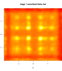
Figure 4: Smoothed $\log\hat{\theta}_{n}(x)$ values, using loess in R with span=0.01, after the first and second stages (reds are lower values), and by a histogram of values from the second stage.

Notice the increase in fidelity from one stage to the next, and the similarity to the predictive error and variance results from Figure 3, with larger lengthscales corresponding to areas poorer emulation under the model with a fixed, global, lengthscale. The final pane in Figure 4 shows a histogram of the $\hat{\theta}_{n}(x)$’s, for $n=50$, obtained after the second stage. The Newton steps from the first stage required about 6.5 iterations on average, with 90% between 6 and 8 whereas the second stage took 4.2 (3 to 6) when primed with previous stage values.

5 Empirical demonstration and comparison

5.1 Illustrative example

We start by making an out-of-sample comparison of our local approximation methods on the prediction problem described above. Comparators include variations based on NN, and greedy selection via MPSE and ALC. All greedy methods are initialized with $\theta_{0}=0.7$ which is in the lower quartile of squared distances in $X$. We furthermore consider a second iteration of MSPE and ALC local design initialized with smoothed MLEs $\hat{\theta}_{n}(x)$ from the first stage. NN with $\hat{\theta}_{n}(x)$ is included too, which we regard as one of our novel (if small) contributions. Note that fully placing NN in the context of the scheme outlined in Section 4 has limits since later stage local NN designs would be identical to those from the first stage, as they do not depend on $\theta$. We consider variations where MLEs are not calculated. In those cases we used $\theta_{0}=1$ which is a reasonable but not optimal value, inside but towards the upper extreme of the 95% interval of $\hat{\theta}_{n}(x)$-values found, ex poste, by the other methods. The timings were obtained with 8 threads on $4$-core hyperthreaded iMac, via OpenMP pragmas. All other particulars are exactly as described by the illustrations above We also consider a “big” NN benchmark, which uses $n=200$. The others used $n=50$, as previously.

Table SM.2 summarizes execution time in seconds, predictive accuracy with RMSE, uncertainty with pointwise 95% intervals, etc. All methods exhibit high precision on the scale of the response, and all over cover. The best methods are three times better than the worst with, generally speaking, more computational effort reaping rewards. Methods which do not infer $\hat{\theta}_{n}(x)$ fare worst, and NN is only competitive with the greedy methods when it uses an order of magnitude larger local designs (“nnbig”). Although competitive in terms of accuracy per unit time, even giving lower predicted standard deviation, this success comes at the expense of storing a 4x larger output object, which may limit portability.

5.2 Comparison to compactly supported covariances

For a broader comparison, consider the borehole function (Worley,, 1987) which is a common benchmark for computer experiments (e.g. Morris et al.,, 1993). The response $y$ is given by

$$y=2\pi T_{u}[H_{u}-H_{l}]\left/\log\left(\frac{r}{r_{w}}\right)\left[1+\frac{2LT_{u}}{\log(r/r_{w})r_{w}^{2}K_{w}}+\frac{T_{u}}{T_{l}}\right]\right.\,.$$ (10)

The eight inputs are constrained to lie in a rectangular domain:

$$r_{w} \in[0.05,0.15] r \in[100,5000] T_{u} \in[63070,115600] T_{l} \in[63.1,116]$$

$$H_{u} \in[990,1110] H_{l} \in[700,820] L \in[1120,1680] K_{w} \in[9855,12045].$$

Part of our reason for choosing this data is that it was used as an illustrative example for the CSC method described by Kaufman et al., (2012), which may be the most widely adopted modern approach to fast approximate emulation for computer experiments. The authors provide a script illustrating their R package sparseEM on this data.

http://www.stat.berkeley.edu/~cgk/rcode/assets/SparseEmExample.R

Here we follow that script verbatim, except augmenting their 99% sparse estimator with a 99.9% one for faster results. They generate a LHS of size $4500$, using the first 4000 for training and the rest for testing, and use a statistic called NSE for evaluation. As we argue in SM§5, raw NSE values can be hard to interpret when measuring the accuracy of deterministic computer experiments, so we instead report report $\sqrt{1-\mathrm{NSE}}=\mathrm{sd}(\mbox{prediction error})/\mathrm{sd}(\mbox{response})$, and in addition to other metrics like RMSE.

	$N=4000$, $N_{\mathrm{pred}}=500$
method	secs	$\sqrt{1-\mathrm{NSE}}$	RMSE	95%c	SD	$p$-val
alc2	46.3	0.0196	0.884	1.000	2.71	0.0776
mspe2	83.8	0.0197	0.889	1.000	2.72	0.0000
nnbig	20.0	0.0225	1.018	0.992	1.41	0.0000
alc	23.5	0.0259	1.172	0.999	2.79	0.4164
mspe	41.9	0.0259	1.172	1.000	2.78	0.0000
csc99	3105.8	0.0309	1.396	0.961	1.47	0.0000
csc999	181.9	0.0337	1.525	0.957	1.54	0.0000
nn	0.5	0.0647	2.920	0.964	2.60	0.0047
mspe.nomle	41.3	0.0673	3.040	0.992	4.77	0.0022
alc.nomle	23.2	0.0681	3.075	0.991	4.79	0.0000
nnbig.nomle	8.8	0.0719	3.246	0.811	2.78	0.0000
nn.nomle	0.2	0.1637	7.388	0.799	5.43

Table 1: Average timings (in seconds) and accuracy (in $\sqrt{1-\mathrm{NSE}}$) values from thirty-fold Monte Carlo experiments on the borehole data. The final column contains $p$-values from one-sided $t$-tests of adjacent performers (better v. next-best). The rows of the Table are ordered by the accuracy estimate(s).

Table 1 summarizes the results of a comparison involving thirty Monte Carlo repetitions, each with new random LHS testing and training sets. Package defaults are used in all cases; second-stage greedy methods (e.g., “mspe2”) used unsmoothed first stage $\theta_{x}=\hat{\theta}_{n}(x)$ values (from “mspe”). The timings, obtained on the same $4$-core hyperthreaded iMac throughout, comprise of the sum of fitting and prediction stages. OpenMP pragmas, with 8 threads, were used to parallelize our local design methods. Although CSC is not explicitly multi-threaded, the sparse linear algebra libraries it uses (from the spam package) are lightly threaded and were observed to utilize between one and five threads in this example. We can see clearly from the table(s) that even without parallelization ($\sim\!8$x slower) our local methods are orders of magnitude faster than the CSC ones.

Differences in the raw accuracy numbers, via average $\sqrt{1-\mathrm{NSE}}$ or RMSE, are much greater than they were in our earlier illustrative example. Acknowledging the randomness in the Monte Carlo setup, the final column gives a $p$-value for a one-sided paired $t$-test under the alternative that that row’s NSE came from a different population than those with the next-lowest averages (next row down). For example, at the 5% level, the best method (“alc2”) is not statistically better than the second best (“mspe2”), whereas both are convincingly better than the third best, and so on. At a high level, observe that the local methods without $\hat{\theta}(x)$ fare worst. NN $(n=50)$ is dominated by greedy methods across the board. Due to lack of statistical significance in differences between MSPE and ALC, the former might not be worth the added computational expense. As before, a big NN ($n=200$) is competitive in terms of accuracy per second, however only when local MLEs are calculated. Without local inference and parallelization (both our contributions), the “big” NN method is amongst the most expensive ($8.8\times 8\approx 70$ secs) and the least accurate.

Focusing on the uncertainty estimates in the table, observe that the greedy methods over cover, whereas the CSCs have the correct nominal pointwise coverage. They also have, with the exception of “nnbig”, lower predicted standard deviation. Interpreting these results is not straightforward, however. The true response is smooth and deterministic, so the 5% which CSC mis-covers must comprise a small number of contiguous regions of the input space where it was (possibly substantially) biased. We therefore draw comfort from the fact that the local methods are both more accurate and more conservative. The low standard deviation of “nnbig” would seem to be due solely to the larger $n$ in the denominator of $\psi_{n}(x)$ in (1), not to a better estimate of the global variance structure. This can be verified by replacing $50\cdot\psi_{n}(x)/200$ in the coverage calculations for the other $n=50$ estimators, which results in values nearly identical to the others. We conclude that our greedy methods are (perhaps overly) conservative. However next to “nn”, which provides deceptively good coverage results, caution in terms of predictive uncertainty pays dividends in accuracy.

Results for a double-sized experiment are shown in Table SM.1. Accuracy results increase slightly, but relative orders are similar. What is noteworthy is that the local methods require, as expected, about double the computational effort. By contrast the CSC methods take four to eight times longer, suggesting a quadratic scaling in $N$. Anecdotally we remark that the 99% sparse CSC method on $(N,n)=(8000,1000)$ approaches the limit of the size of problem possible on this machine due to memory constraints. We tried $N=10000$. Frequent memory pages to disk lead to dramatic slowdowns; our estimates suggest the code would have taken days to finish. By contrast, the local/greedy methods required seconds more.

6 Discussion

We outlined a family of sequential design schemes to modernize an old idea of approximate kriging based on local neighborhoods [for a recent reference, see Emory, (2009)]. The result is a predictor that is fast, nonstationary, highly parallelizable, and whose “knobs” offer direct control on speed versus accuracy. Really the only tuning parameter is $n$. We argue in favor of calculating local designs which differ from a simpler (yet modernized) NN, and give two greedy algorithms which have the same local $O(n^{3})$ computational order as NN. But the order notation hides large constant, which means that the greedy methods demand compute cycles that could have been spent, e.g., by NN with a larger $n$ budget. Indeed, our results show that this approach is competitive, but not without modern enhancements like local $\hat{\theta}_{n}(x)$ and parallel computation. Nevertheless, instinct suggests that smaller $n$ is better. Many of our ideas for extension, which we outline below, bear this out.

By saving a small amount of information—indices of the local designs at each $x$, and corresponding $\hat{\theta}_{n}(x)$ values—designs can augmented, picking up where they left off if more compute cycles become available. Those resources do not need to be allocated uniformly. Larger local designs $n(x)$ can be sought where, e.g., the potential to reduce variance or increase accuracy is larger. Such decisions can be made more judiciously (i.e., accurately, via ALC) and efficiently (smaller $n$ calculations) under a greedy local design scheme, compared to NN say. This is suggestive of benefit from differential effort through the stages of global inference in Section 4.2. One could start with a small $n$ and local inference based on NN; then iterate with ALC and/or MSPE, possibly increasing $n$; and finally allocate additional $n(x)$, refining hard-to-predict areas until the computing budget is exhausted.

Having a stopping criterion might be desirable when computational limits are less constrained, which when applied independently to obtain $n_{\mathrm{thresh}}(x)$ for each $x$ could represent an alternative mechanism for allocating computational resources differentially amongst the predictive locations. One option is to track the ratio of predictive and reduced variances ($V_{j}(x)/V_{j+1}(x)$) over the iterations, and stop beyond a certain minimum threshold. Both depend on $\psi_{j}$, so cancellation would lead to a metric independent of the responses $\{y_{i}\}_{i=1}^{j}$ (other than via a common estimate of $\theta$). However, non-uniform full-data designs coupled with spatially varying choices for $\theta$ make the actual time to convergence—which is related cubically to $n_{\mathrm{thresh}}(x)$—highly unpredictable. Since lack of predictability would be compounded over thousands of independent local searches, practical considerations may necessitate a low global cap on $n_{\mathrm{thresh}}(x)$, recommending against a simplistic NN approach.

We remark that there is a trade-off between the size of local designs and the non-stationary flexibility of the global predictor: as the designs get larger, the global surface can exhibit less spatial heterogeneity. With larger $n$, approximation will improve relative to the full-data GP, but it may exhibit poorer out-of-sample performance, suggesting it could be beneficial to stop early. Post-process pruning steps, perhaps via an out-of-sample validation scheme, could be deployed to find $n^{*}(x)\leq n$, a search which is more efficient the smaller $n$ is to start with. Another option is to augment the GP with elaborate mean structure, following Kaufman et al., (2012). That would allow a sparser covariance structure, which for us is a sparser local design (again smaller $n$). That mean structure is one of the big strengths of the CSC method, which we anticipate would fare better than ours in extrapolation exercises, or when predicting in an area of of the input space with very sparse design coverage.

When the design and predictive grids are dense, and when the same $\theta$ parameters are used globally, the pattern of greedy local designs in the interior of the input space (away from the boundaries) are highly regular. For example, Figure 1 suggests a simple template-based rule (e.g., some NNs and some farther out) may be a thrifty alternative to expensive MSPE/ALC calculation. Along similar lines, we have found that substantial speedups can be obtained by searching first over the closest members of $X-X_{j}(x)$. One option is to stop early once some tolerance is reached on changes to ALC/MSPE. Even simpler is to restrict searches to a more modestly sized local neighborhood of candidates $N^{\prime}\ll N$, say $N^{\prime}=n^{m}$ for $m$-dimensional input spaces. Actually, for all experiments in this paper, we restricted searches to the nearest $N^{\prime}=$1000 candidates. Results (except time) with $N^{\prime}=10000$.

We envision further potential benefits from parallelization. Numbers of desktop computing cores are doubling every few years and our methods are well-positioned to take advantage. Graphical processing units (GPUs) are taking off for scientific computing, having thousands of stripped-down computing cores. An early early GPU version of ALC–based local design search has yielded 20–70x efficiency gains (Gramacy et al.,, 2013).

Finally, we anticipate that a modern local approach to GP emulation will have applicability beyond emulation. For example, they may be ideal for computer model calibration where predictions are only required over part of the input space: at pairings of the calibration parameter(s) with a small number of field data sites. In that case it might be sensible to build “local” designs jointly for field data locations. Although the details for doing this by MSPE are still under development, an ALC version can be invoked by providing a matrix of $x$-values to the laGP function in the R package. Other contexts clearly pose challenges for local emulation. For example, when optimizing black box functions by expected improvement—where designs ($N$) are small and predictive grids are potentially enormous.

Acknowledgments

The authors would like to thank Jarad Niemi for thoughtful discussions on early drafts, and Brian Williams for a careful proofing of our mathematical appendices. We would also like to thank two referees and an AE for constructive criticism on our initial submission. This work was supported in part by NSF grant number CMMI-1233403.

Supplementary Materials

SM§1 Partition inverse equations

Barnett, (1979) gives the following decomposition.

If $$K(x) =\begin{bmatrix}K&k(x)\\ k^{\top}(x)&K(x,x)\end{bmatrix}, K^{-1}(x) =\begin{bmatrix}[K^{-1}+g(x)g^{\top}(x)v(x)]&g(x)\\ g^{\top}(x)&v^{-1}(x)\end{bmatrix},$$ then

where $g(x)=-v^{-1}(x)K^{-1}k(x)$ and $v(x)=K(x,x)-k^{\top}(x)K^{-1}k(x)$.

SM§2 Mean-squared predictive error

Here we derive the expressions behind the MSPE (4) development in Section 3. We allow any form of the correlation function where derivatives are analytic. Although our expressions in the main body of text assume a scalar parameter $\theta$, the derivations here allow for a $p$-parameter family, where $p\geq 1$. Therefore our partial derivatives are expressed component-wise and vectorized as appropriate. In most cases, the single-parameter result is obtained straightforwardly by removing subscripts and collapsing products of identical second derivatives into squares and/or factors of two.

We begin with the batch log likelihood derivatives which lead to the Fisher information. Define $w_{j}=K^{-1}_{j}Y_{j}$, which is a component of the marginal (log) likelihood (1) for data $D_{j}$ via $\psi_{j}$. Much of what follows repeatedly leverages that

$$\frac{\partial K_{j}^{-1}}{\partial\theta_{k}}=-K_{j}^{-1}\frac{\partial K_{j}}{\partial\theta_{k}}K_{j}^{-1},$$ (SM.1)

where $\frac{\partial K_{j}}{\partial\theta_{k}}$ is the matrix of partial derivatives corresponding to $K_{j}$ calculated via $K_{\theta,\eta}(x,x^{\prime})$ for all $(x,x^{\prime})$ pairs in $D_{j}$. Recursive application yields $\frac{\partial^{2}K_{j}}{\partial\theta_{k}\partial\theta_{l}}$. Then, for $1\leq k,l\leq p$, we have

$$\frac{\partial w_{j}}{\partial\theta_{k}} =-K_{j}^{-1}\frac{\partial K_{j}}{\partial\theta_{k}}w_{j}, \mbox{and }\;\;\;\frac{\partial^{2}w_{j}}{\partial\theta_{k}\partial\theta_{l}} =-K_{j}^{-1}\left[\frac{\partial^{2}K_{j}}{\partial\theta_{k}\partial\theta_{l}}w_{j}+\frac{\partial K_{j}}{\partial\theta_{k}}\frac{\partial w_{j}}{\partial\theta_{l}}+\frac{\partial K_{j}}{\partial\theta_{l}}\frac{\partial w_{j}}{\partial\theta_{k}}\right].$$ (SM.2)

Also useful is

$$\frac{\partial\log|K_{j}|}{\partial\theta_{k}}=\frac{1}{|K_{j}|}\frac{\partial|K_{j}|}{\partial\theta_{k}}=\frac{|K_{j}|\,\mathrm{tr}\!\left\{K_{j}^{-1}\frac{\partial K_{j}}{\partial\theta_{k}}\right\}}{|K_{j}|}=\mathrm{tr}\!\left\{K_{j}^{-1}\frac{\partial K_{j}}{\partial\theta_{k}}\right\}.$$

Note that the trace of a product of square matrices $M^{(1)}$ and $M^{(2)}$ may be efficiently computed as $\sum_{k,l}M^{(1)}_{lk}M^{(2)}_{kl}$.

Using the above results, the first and second derivatives of the log likelihood $\ell_{j}(\theta)\equiv\log p(Y_{j}|\theta,X_{j})$ given in (1) are (for $1\leq k,l\leq p$)

$$\frac{\partial\ell_{j}(\theta)}{\partial\theta_{k}} =-\frac{1}{2}\,\mathrm{tr}\!\left\{K_{j}^{-1}\frac{\partial K_{j}}{\partial\theta_{k}}\right\}+\frac{jY_{j}^{\top}K_{j}^{-1}\frac{\partial K_{j}}{\partial\theta_{k}}K_{j}^{-1}Y_{j}}{2\psi_{j}},$$

$$\mbox{and }\;\;\;\frac{\partial^{2}\ell_{j}(\theta)}{\partial\theta_{k}\partial\theta_{l}} =-\frac{1}{2}\,\mathrm{tr}\!\left\{K_{j}^{-1}\left[\frac{\partial^{2}K_{j}}{\partial\theta_{k}\partial\theta_{l}}-\frac{\partial K_{j}}{\partial\theta_{l}}K_{j}^{-1}\frac{\partial K_{j}}{\partial\theta_{k}}\right]\right\}$$

$$\;\;\;-\frac{jY^{\top}K_{j}^{-1}}{2\psi_{j}}\left[2\frac{\partial K_{j}}{\partial\theta_{l}}K_{j}^{-1}\frac{\partial K_{j}}{\partial\theta_{k}}-\frac{\partial^{2}K_{j}}{\partial\theta_{k}\partial\theta_{l}}\right]K_{j}^{-1}Y_{j}$$

$$\;\;\;+\frac{j}{2\psi_{j}^{2}}\left(Y_{j}^{\top}K_{j}^{-1}\frac{\partial K_{j}}{\partial\theta_{k}}K_{j}^{-1}Y_{j}\right)\left(Y_{j}^{\top}K_{j}^{-1}\frac{\partial K_{j}}{\partial\theta_{l}}K_{j}^{-1}Y_{j}\right).$$

The Fisher information $F_{j}(\theta)$ matrix is obtained by negating the $(k,l)$ elements of the second derivative above. Some simplifications arise in the the one-dimensional parameter case, which we quote below for easy reference when following the development in the main manuscript.

$$\ell^{\prime}(\theta) \equiv\frac{\partial\log p(Y|K)}{\partial\theta}=-\frac{1}{2}\mathrm{tr}\left\{K^{-1}\dot{K}\right\}+\frac{N}{2}\times\frac{(Y^{\top}K^{-1}\dot{K}K^{-1}Y)}{\psi},$$ (SM.3)

$$\ell^{\prime\prime}(\theta) \equiv\frac{\partial^{2}\log p(Y|K)}{\partial^{2}\theta}=-\frac{1}{2}\mathrm{tr}\left\{K^{-1}\left[\ddot{K}-\dot{K}K^{-1}\dot{K}\right]\right\}$$ (SM.4)

$$+\frac{N}{2\psi}\times Y^{\top}K^{-1}\left[\ddot{K}-2\dot{K}K^{-1}\dot{K}\right]K^{-1}Y+\frac{N}{2\psi^{2}}\times\left[Y^{\top}K^{-1}\dot{K}K^{-1}Y\right]^{2},$$

where $\dot{K}$ and $\ddot{K}$ are shorthand for $\frac{\partial K}{\partial\theta}$ and $\frac{\partial^{2}K}{\partial^{2}\theta}$ respectively.

Sequential updating of the Fisher information leverages a recursive expression of the log likelihood which follows trivially from a cascading conditional representation of the joint probability of the responses given the parameters $\ell_{j+1}(\theta)=\log p(Y_{j+1}|\theta)=\log p(Y_{j}|\theta)+\log p(y_{j+1}|Y_{j},\theta)\equiv\ell_{j}(\theta)+\ell_{j}(y_{j+1};\theta)$ where the final term represents the conditional log-likelihood for $y_{j+1}$ given $Y_{j}$ and $\theta$. Taking (negative) second derivatives yields the following updating equations

$$\left\{F_{j+1}(\theta)\right\}_{kl}=-\frac{\partial^{2}\ell_{j}(\theta)}{\partial\theta_{k}\partial\theta_{l}}-\frac{\partial\ell_{j}(y_{j+1};\theta)}{\partial\theta_{k}\partial\theta_{l}}=\{F_{j}(\theta)\}_{kl}-\frac{\partial\ell_{j}(y_{j+1};\theta)}{\partial\theta_{k}\partial\theta_{l}}$$

Deriving the final term, here, requires expressions for $y_{t+1}|Y_{t},\theta$, i.e., the predictive equations, and their derivatives. First,

$$\ell_{j}(y_{t+1};\theta) =\mbox{const }-\frac{1}{2}\log V_{j}(x_{j+1};\theta)-\left(\frac{j+1}{2}\right)\log\left[j-2+\frac{(y_{j+1}-\mu_{j}(x_{j+1};\theta))^{2}}{V_{j}(x_{j+1};\theta)}\right]$$

$$\equiv\mbox{const }-\frac{1}{2}\log V_{j}-\left(\frac{j+1}{2}\right)\log\left[j-2+\frac{(y_{j+1}-\mu_{j})^{2}}{V_{j}}\right],$$

thereby defining some shorthand that will be useful going forward.

The derivatives of the log likelihood follow immediately from applications of the chain rule. For $1\leq k,l\leq p$,

$$\frac{\partial\ell_{j}(y_{j+1};\theta)}{\partial\theta_{k}}=-\frac{1}{2V_{j}}\frac{\partial V_{j}}{\partial\theta_{k}}+\left(\frac{j+1}{2}\right)\left[j-2+\frac{(y_{j+1}-\mu_{j})^{2}}{V_{j}}\right]^{-1}$$ (SM.5)

$$\;\;\;\;\times\left[\frac{2(y_{j+1}-\mu_{j})}{V_{j}}\frac{\partial\mu_{j}}{\partial\theta_{k}}+\frac{(y_{j+1}-\mu_{j})^{2}}{V_{j}^{2}}\frac{\partial V_{j}}{\partial\theta_{k}}\right].$$

$$\frac{\partial^{2}\ell_{j}(y_{j+1};\theta)}{\partial\theta_{k}\partial\theta_{l}}=-\frac{1}{2V_{j}}\frac{\partial^{2}V_{j}}{\partial\theta_{k}\partial\theta_{l}}+\frac{1}{2V_{j}^{2}}\frac{\partial V_{j}}{\partial\theta_{k}}\frac{\partial V_{j}}{\partial\theta_{l}}+\left(\frac{j+1}{2}\right)\left[j-2+\frac{(y_{j+1}-\mu_{j})^{2}}{V_{j}}\right]^{-2}$$ (SM.6)

$$\;\;\;\;\times\left[\frac{2(y_{j+1}-\mu_{j})}{V_{j}}\frac{\partial\mu_{j}}{\partial\theta_{k}}+\frac{(y_{j+1}-\mu_{j})^{2}}{V_{j}^{2}}\frac{\partial V_{j}}{\partial\theta_{k}}\right]\left[\frac{2(y_{j+1}-\mu_{j})}{V_{j}}\frac{\partial\mu_{j}}{\partial\theta_{l}}+\frac{(y_{j+1}-\mu_{j})^{2}}{V_{j}^{2}}\frac{\partial V_{j}}{\partial\theta_{l}}\right]$$

$$\;\;\;\;+\left(\frac{j+1}{2}\right)\left[j-2+\frac{(y_{j+1}-\mu_{j})^{2}}{V_{j}}\right]^{-1}\left\{-\frac{2}{V_{j}}\frac{\partial\mu_{j}}{\partial\theta_{k}}\frac{\partial\mu_{j}}{\partial\theta_{l}}-\frac{2(y_{j+1}-\mu_{j})}{V_{j}^{2}}\left[\frac{\partial\mu_{j}}{\partial\theta_{k}}\frac{\partial V_{j}}{\partial\theta_{l}}+\frac{\partial\mu_{j}}{\partial\theta_{l}}\frac{\partial V_{j}}{\partial\theta_{k}}\right]\right.$$

$$\;\;\;\;\left.+\frac{2(y_{j+1}-\mu_{j})}{V_{j}}\frac{\partial^{2}\mu_{j}}{\partial\theta_{k}\partial\theta_{l}}-\frac{2(y_{j+1}-\mu_{j})^{2}}{V_{j}^{3}}\frac{\partial V_{j}}{\partial\theta_{k}}\frac{\partial V_{j}}{\partial\theta_{l}}+\frac{(y_{j+1}-\mu_{j})^{2}}{V_{j}^{2}}\frac{\partial^{2}V_{j}}{\partial\theta_{k}\partial\theta_{l}}\right\}$$

Eqs. (SM.5–SM.6) require the derivatives of the predictive equations. In turn, those require $w_{j}$ and its derivatives (SM.2), and a new quantity $z_{j}=K_{j}^{-1}k_{j}\equiv K_{j}^{-1}k_{j}(x_{j+1};\theta)$ and its derivatives:

$$\frac{\partial z_{j}}{\partial\theta_{k}} =K_{j}^{-1}\left[\frac{\partial k_{j}}{\partial\theta_{k}}-\frac{\partial K_{j}}{\partial\theta_{k}}z_{j}\right],$$ (SM.7)

$$\mbox{and }\;\;\;\frac{\partial^{2}z_{j}}{\partial\theta_{k}\partial\theta_{l}} =K_{j}^{-1}\left[\frac{\partial^{2}k_{j}}{\partial\theta_{k}\partial\theta_{l}}-\frac{\partial^{2}K_{j}}{\partial\theta_{k}\partial\theta_{l}}z_{j}-\frac{\partial K_{j}}{\partial\theta_{k}}\frac{\partial z_{j}}{\partial\theta_{l}}-\frac{\partial K_{j}}{\partial\theta_{l}}\frac{\partial z_{j}}{\partial\theta_{k}}\right]$$ (SM.8)

which follow from applications of (SM.1). The derivatives of the mean are then revealed as

$$\frac{\partial\mu_{j}}{\partial\theta_{k}} =\frac{\partial z_{j}^{\top}}{\partial\theta_{k}}Y_{j}, \frac{\partial^{2}\mu_{j}}{\partial\theta_{k}\partial\theta_{l}} =\frac{\partial^{2}z_{j}^{\top}}{\partial\theta_{k}\partial\theta_{l}}Y_{j}.$$ and (SM.9)

For the variances it helps to write $V_{j}=\frac{1}{j-2}\times\psi_{j}\times v_{j}$ where $v_{j}\equiv v_{j}(x_{j+1};\theta)=K_{\eta}(x_{j+1},x_{j+1})-k_{j}^{\top}(x_{j+1})K_{j}^{-1}k_{j}(x_{j+1})$, and $\psi_{j}\equiv\psi_{j}(\theta)$. We assume that when the arguments to $K_{\theta,\eta}$ are identical, as in $v_{j}$, the correlation function is no longer a function of $\theta$. Derivatives then follow as

$$\frac{\partial V_{j}}{\partial\theta_{k}} =\left(\frac{1}{j-2}\right)\left[\frac{\partial\psi_{j}}{\partial\theta_{k}}v_{j}+\psi_{j}\frac{\partial v_{j}}{\partial\theta_{k}}\right]$$

$$=\left(\frac{1}{j-2}\right)\left[Y_{j}^{\top}\frac{\partial w_{j}}{\partial\theta_{k}}v_{j}-\psi_{j}\left(\frac{\partial k_{j}^{\top}}{\partial\theta_{k}}z_{j}+k_{j}^{\top}\frac{\partial z_{j}}{\partial\theta_{k}}\right)\right],\;\;\;\mbox{ and}$$ (SM.10)

$$\frac{\partial^{2}V_{j}}{\partial\theta_{k}\partial\theta_{l}} =\left(\frac{1}{j-2}\right)\left\{Y_{j}^{\top}\frac{\partial^{2}w_{j}}{\partial\theta_{k}\partial\theta_{l}}v_{j}+Y_{j}^{\top}\frac{\partial w_{j}}{\partial\theta_{k}}\frac{\partial v_{j}}{\partial\theta_{l}}-\frac{\partial\psi_{j}}{\partial\theta_{l}}\left[\frac{\partial k_{j}^{\top}}{\partial\theta_{k}}z_{j}+k_{j}^{\top}\frac{\partial z_{j}}{\partial\theta_{k}}\right]\right.$$

$$\;\;-\left.\psi_{j}\left[\frac{\partial^{2}k_{j}^{\top}}{\partial\theta_{k}\partial\theta_{l}}z_{j}+\frac{\partial k_{j}^{\top}}{\partial\theta_{k}}\frac{\partial z_{j}}{\partial\theta_{l}}+\frac{\partial k_{j}^{\top}}{\partial\theta_{l}}\frac{\partial z_{j}}{\partial\theta_{k}}+k_{j}^{\top}\frac{\partial^{2}z_{j}}{\partial\theta_{k}\partial\theta_{l}}\right]\right\}$$

$$=\left(\frac{1}{j-2}\right)\left\{Y_{j}^{\top}\frac{\partial^{2}w_{j}}{\partial\theta_{k}\partial\theta_{l}}v_{j}-Y_{j}^{\top}\frac{\partial w_{j}}{\partial\theta_{k}}\left[\frac{\partial k_{j}^{\top}}{\partial\theta_{l}}z_{j}+k_{j}^{\top}\frac{\partial z_{j}}{\partial\theta_{l}}\right]\right.$$ (SM.11)

$$\;\;-Y_{j}^{\top}\frac{\partial w_{j}}{\partial\theta_{l}}\left[\frac{\partial k_{j}^{\top}}{\partial\theta_{k}}z_{j}+k_{j}^{\top}\frac{\partial z_{j}}{\partial\theta_{k}}\right]\left.-\,\psi_{j}\!\left[\frac{\partial^{2}k_{j}^{\top}}{\partial\theta_{k}\partial\theta_{l}}z_{j}+\frac{\partial k_{j}^{\top}}{\partial\theta_{k}}\frac{\partial z_{j}}{\partial\theta_{l}}+\frac{\partial k_{j}^{\top}}{\partial\theta_{l}}\frac{\partial z_{j}}{\partial\theta_{k}}+k_{j}^{\top}\frac{\partial^{2}z_{j}}{\partial\theta_{k}\partial\theta_{l}}\right]\right\}.$$

This completes the expressions required for updating the Fisher information matrix.

The MSPE calculation (4) requires that the conditional likelihood be replaced with the expectation

$$\mathcal{G}_{j+1}(\theta)=F_{j}(\theta)+\mathbb{E}\left\{-\frac{\partial^{2}\ell_{j}(y_{j+1};\theta)}{\partial\theta_{k}\partial\theta_{l}}\right\}$$

because we wish to select the next $x_{j+1}$ in a manner that does not utilize the “future” observation $y_{j+1}$. Unfortunately, the Student-$t$ predictive equations (2–3) preclude a tractable analytic expectation calculation. Therefore, we approximate by employing Gaussian surrogate equations with matched moments. I.e.,

$$\ell_{j}(y_{j+1};\theta)=\log p(y_{j+1}|Y_{j},\theta)\approx-\frac{1}{2}\log{2\pi}-\frac{1}{2}\log V_{j}-\frac{(y_{j+1}-\mu_{j})^{2}}{2V_{j}}.$$ (SM.12)

The (exact) derivatives for the approximation (SM.12) then follow, for $1\leq k,l,\leq p$

$$\frac{\partial\ell_{j}(y_{j+1};\theta)}{\partial\theta_{k}} \approx-\frac{1}{2V_{j}}\frac{\partial V_{j}}{\partial\theta_{k}}+\frac{(y_{j+1}-\mu_{j})}{V_{j}}\frac{\partial\mu_{j}}{\partial\theta_{k}}+\frac{(y_{j+1}-\mu_{j})^{2}}{2V_{j}^{2}}\frac{\partial V_{j}}{\partial\theta_{k}},$$ (SM.13)

$$\mbox{and }\;\;\frac{\partial^{2}\ell_{j}(y_{j+1};\theta)}{\partial\theta_{k}\partial\theta_{l}} \approx-\frac{1}{2V_{j}}\frac{\partial^{2}V_{j}}{\partial\theta_{k}\partial\theta_{l}}+\frac{1}{2V_{j}^{2}}\frac{\partial V_{j}}{\partial\theta_{k}}\frac{\partial V_{j}}{\partial\theta_{l}}-\frac{1}{V_{j}}\frac{\partial\mu_{j}}{\partial\theta_{k}}\frac{\partial\mu_{j}}{\partial\theta_{l}}$$ (SM.14)

$$\;\;\;+\frac{(y_{j+1}-\mu_{j})}{V_{j}}\frac{\partial^{2}\mu_{j}}{\partial\theta_{k}\partial\theta_{l}}-\frac{(y_{j+1}-\mu_{j})}{V_{j}^{2}}\left[\frac{\partial\mu_{j}}{\partial\theta_{k}}\frac{\partial V_{j}}{\partial\theta_{l}}+\frac{\partial V_{j}}{\partial\theta_{k}}\frac{\partial\mu_{j}}{\partial\theta_{l}}\right]$$

$$\;\;\;+\frac{(y_{j+1}-\mu_{j})^{2}}{2V_{j}^{2}}\frac{\partial^{2}V_{j}}{\partial\theta_{k}\partial\theta_{l}}-\frac{(y_{j+1}-\mu_{j})^{2}}{V_{j}^{3}}\frac{\partial V_{j}}{\partial\theta_{k}}\frac{\partial V_{j}}{\partial\theta_{l}}.$$

Taking the (negative) expectation of (SM.14) gives,

$$\mathbb{E}\left\{-\frac{\partial^{2}\ell_{j}(y_{j+1};\theta)}{\partial\theta_{k}\partial\theta_{l}}\Big{|}Y_{j},\theta\right\} =\frac{1}{2V_{j}}\frac{\partial^{2}V_{j}}{\partial\theta_{k}\partial\theta_{l}}-\frac{1}{2V_{j}^{2}}\frac{\partial V_{j}}{\partial\theta_{k}}\frac{\partial V_{j}}{\partial\theta_{l}}+\frac{1}{V_{j}}\frac{\partial\mu_{j}}{\partial\theta_{k}}\frac{\partial\mu_{j}}{\partial\theta_{l}}$$

$$\;\;\;-\frac{1}{2V_{j}}\frac{\partial^{2}V_{j}}{\partial\theta_{k}\partial\theta_{l}}+\frac{1}{V_{j}^{2}}\frac{\partial V_{j}}{\partial\theta_{k}}\frac{\partial V_{j}}{\partial\theta_{l}}$$

$$=\frac{1}{2V_{j}^{2}}\frac{\partial V_{j}}{\partial\theta_{k}}\frac{\partial V_{j}}{\partial\theta_{l}}+\frac{1}{V_{j}}\frac{\partial\mu_{j}}{\partial\theta_{k}}\frac{\partial\mu_{j}}{\partial\theta_{l}}$$ (SM.15)

Now, given a specified input site $x$ at which predictions of $Y(x)$ are desired, and given data $D_{j}$ containing previously selected sites, the objective is to choose the next site $x_{j+1}$ recognizing that the data pairs will lead to improved predictions via (2–3) and an improved estimate of the correlation parameters $\theta$. If the latter were of primary concern, one possible way to choose $x_{j+1}$ would be to maximize the determinant of $\mathcal{G}_{j+1}(\theta)$ for some choice of $\theta$. While reasonable, this does not directly consider the prediction error variance of $Y(x)$. Therefore it possess no mechanism for giving a local character to the estimate of $\theta$. So instead we propose to choose $x_{j+1}$ to minimize the predictive variance of $Y(x)$ in a manner that considers the impact of estimation uncertainty in $\theta$. Specifically, we choose $x_{j+1}$ to minimize the Bayesian mean squared prediction error defined as

$$J(x_{j+1},x)=\mathbb{E}\left\{\left[Y(x)-\mu_{j+1}(x;\hat{\theta}_{j+1})\right]^{2}\Big{|}Y_{j}\right\},$$ (SM.16)

where $\mu_{j+1}(x;\hat{\theta}_{j+1})$ depends on $(x_{j+1},y_{j+1})$ and represents the hypothetical prediction of $Y(x)$ that would result after choosing $x_{j+1}$, observing $y_{j+1}$, calculating MLE $\hat{\theta}_{j+1}$ based on the expanded data set $D_{j+1}$, and using the MLE in the prediction of $Y(x)$. Eq. (SM.16) becomes

$$J(x_{j+1},x) =\mathbb{E}\left\{\left[Y(x)-\mu_{j+1}(x;\theta)+\mu_{j+1}(x;\theta)-\mu_{j+1}(x;\hat{\theta}_{j+1})\right]^{2}\Big{|}Y_{j}\right\}$$

$$=\mathbb{E}\left\{\mathbb{E}\left\{\left[Y(x)-\mu_{j+1}(x;\theta)+\mu_{j+1}(x;\theta)-\mu_{j+1}(x;\hat{\theta}_{j+1})\right]^{2}\Big{|}Y_{j},y_{j+1},\theta\right\}\Big{|}Y_{j}\right\}$$

$$=\mathbb{E}\left\{\mathbb{E}\left\{\left[Y(x)-\mu_{j+1}(x;\theta)\right]^{2}\Big{|}Y_{j},y_{j+1},\theta\right\}\Big{|}Y_{j}\right\}$$

$$\;\;\;+2\mathbb{E}\left\{\mathbb{E}\left\{\left[Y(x)-\mu_{j+1}(x;\theta)\right]\left[\mu_{j+1}(x;\theta)-\mu_{j+1}(x;\hat{\theta}_{j+1})\right]\Big{|}Y_{j},y_{j+1},\theta\right\}\Big{|}Y_{j}\right\}$$

$$\;\;\;+\mathbb{E}\left\{\mathbb{E}\left\{\left[\mu_{j+1}(x;\theta)-\mu_{j+1}(x;\hat{\theta}_{j+1})\right]^{2}\Big{|}Y_{j},y_{j+1},\theta\right\}\Big{|}Y_{j}\right\}$$

$$=\mathbb{E}\left\{V_{j+1}(x;\theta)\Big{|}Y_{j}\right\}+0+\mathbb{E}\left\{\left[\mu_{j+1}(x;\theta)-\mu_{j+1}(x;\hat{\theta}_{j+1})\right]^{2}\Big{|}Y_{j}\right\}.$$ (SM.17)

Regarding the first term in (SM.17), we write it as

$$\mathbb{E}\left\{V_{j+1}(x;\theta)\Big{|}Y_{j}\right\}=\mathbb{E}\left\{\frac{\psi_{j}(\theta)}{(j-1)}v_{j+1}(x;\theta)\Big{|}Y_{j}\right\} =\frac{\psi_{j}(\theta)}{j-2}v_{j+1}(x;\theta)$$ (SM.18)

$$\approx\frac{\psi_{j}}{j-2}v_{j+1}(x;\hat{\theta}_{j})$$

which is the new/reduced variance (8) after adding $x_{j+1}$ into $D_{j}$, marginalized with respect to the unknown $y_{j+1}$. The last approximate equality in (SM.18) results from substituting the unknown $\theta$ by its estimate calculated form $D_{j}$. The second equality in (SM.18) follows readily from Eq. (9), which can be written as (omitting $\theta$ for brevity)

$$\psi_{j+1} =\psi_{j}+\frac{\mu_{j}^{2}(x_{j+1})}{v_{j}(x_{j+1})}-\frac{2y_{j+1}\mu_{j}(x_{j+1})}{v_{j}(x_{j+1})}+\frac{y_{j+1}^{2}}{v_{j}(x_{j+1})}=\psi_{j}+\frac{[y_{j+1}-\mu_{j}(x_{j+1})]^{2}}{v_{j}(x_{j+1})},$$

so that

$$\mathbb{E}\{\psi_{j+1}|Y_{j}\} =\psi_{j}+\frac{V_{j}(x_{j+1})}{v_{j}(x_{j+1})}=\psi_{j}+\frac{\psi_{j}v_{j}(x_{j+1})}{(j-2)v_{j}(x_{j+1})}=\frac{(j-1)\psi_{j}}{(j-2)}.$$

Regarding the last term in (SM.17), we again approximate as follows.

$$\mu_{j+1}(x;\theta)-\mu_{j+1}(x;\hat{\theta}_{j+1}) \approx\left[\frac{\partial\mu_{j+1}(x;\theta)}{\partial\theta}\Big{|}_{\theta=\hat{\theta}_{j+1}}\right]^{\top}(\theta-\hat{\theta}_{j+1})$$

$$\approx\left[\frac{\partial\mu_{j}(x;\theta)}{\partial\theta}\Big{|}_{\theta=\hat{\theta}_{j}}\right]^{\top}(\theta-\hat{\theta}_{j+1})$$ (SM.19)

The last inequality in (SM.19) involves two approximations. First, the partial derivative of $\mu_{j+1}(x;\theta)$ at future $\hat{\theta}_{j+1}$ is approximated by the partial derivative at the current $\hat{\theta}_{j}$. The second approximation uses the partial derivative of $\mu_{j}(x;\theta)$ instead. Both are required for tractability because $\hat{\theta}_{j+1}$ and $\mu_{j+1}(x,\theta)$ depend on the future $y_{j+1}$ in a manner that would make the expectation in (SM.18) difficult to evaluate analytically.

Note that the difference between $\mu_{j+1}(x;\theta)$ and $\mu_{j}(x,\theta)$, and their partial derivatives at a common value of $\theta$, will generally be similar for larger $j$ because the most influential points are included in initial iterations. For situations in which $y_{t+1}$ is available in advance, one might consider using it for calculating the partial derivative of $\mu_{j+1}(x;\theta)$, and thereby avoid an approximated expectation. However, even though this would lend tractability and accuracy in one sense, it may not be as attractive a criterion as using $\mu_{j}(x,\theta)$. A strategy that used the partial derivative of $\mu_{j+1}(x;\theta)$ might avoid adding a site at which $y_{j+1}$ was not consistent with the other $\{y_{i},i=1,2,\dots,j\}$, which would ignore unusual or unpredictable features of the response surface.

Substituting (SM.18) and (SM.19) into (SM.17), and assuming the posterior covariance matrix of $\theta$ about its MLE can be approximated by the inverse of the Fisher information matrix $\mathcal{G}_{j+1}(\hat{\theta}_{j})$ given in (4), leaves us with

$$J(x_{j+1},x) =\frac{\psi_{j}}{j-2}v_{j+1}(x;\hat{\theta}_{j})$$

$$\;\;\;+\mathbb{E}\left\{\left[\frac{\partial\mu_{j}(x;\theta)}{\partial\theta}\Big{|}_{\theta=\hat{\theta}_{j}}\right]^{\top}(\theta-\hat{\theta}_{j+1})(\theta-\hat{\theta}_{j+1})^{\top}\left[\frac{\partial\mu_{j}(x;\theta)}{\partial\theta}\Big{|}_{\theta=\hat{\theta}_{j}}\right]\Big{|}Y_{j}\right\}$$

$$\approx\frac{\psi_{j}}{j-2}v_{j+1}(x;\hat{\theta}_{j})+\left[\frac{\partial\mu_{j}(x;\theta)}{\partial\theta}\Big{|}_{\theta=\hat{\theta}_{j}}\right]^{\top}\mathcal{G}_{j+1}^{-1}(\hat{\theta}_{j})\left[\frac{\partial\mu_{j}(x;\theta)}{\partial\theta}\Big{|}_{\theta=\hat{\theta}_{j}}\right].$$

SM§3 Comparison of condition numbers for local designs

A knock-on effect of the spacing of the sub-design points found by the greedy method is that the condition numbers (ratio of the largest to smallest eigenvalue) of the resulting covariance matrices, $K_{j}$, are lower relative to those of the NN method as $j$ becomes large.

Figure SM.1: Condition numbers, kappa$(K_{j}^{-1})/\mbox{\tt dim}(K_{j}^{-1})^{2}$, versus design size, $j$, for NN and greedy methods for two different values of the nugget, $\eta$.

Figure SM.1 provides an illustration. The left plot corresponds to exactly the setup giving rise to the right panel in Figure 1, using ALC; whereas the right plot uses a smaller nugget value, $\eta$. Lower condition numbers indicate greater numerical stability and thus more reliable matrix decompositions. This is relevant for GP surrogate modeling since it means that smaller nuggets, and thus truer interpolations, can be achieved with the greedy method if so desired. Although some recent papers have argued that the quest for truer interpolation in surrogate modeling may not be efficient from a statistical perspective (Gramacy and Lee,, 2011a; Peng and Wu,, 2012), seeking out the smallest possible nugget while retaining numerical stability remains an aspiration in the literature (Ranjan et al.,, 2011).

SM§4 An interpretation of the reduction in variance criterion in terms of partial correlations

The ALC criterion (8) has a helpful interpretation in terms of the partial correlation between the prediction errors at $x$ and at some $x^{\prime}$, a potential new site to be added into the design. For the case when all parameters are known, denote the error in predicting $Y(x)$, given data $D_{j}$, by $e(x|Y_{j})=Y(x)-\mu_{j}(x;\theta)$. Note that $e(x|Y_{j})$ and $Y_{j}$ are orthogonal under the standard correlation inner product, and consider the orthogonal decomposition

$$Y(x)=\mu_{j}(x;\theta)+e(x|Y_{j})=\mu_{j}(x;\theta)+\rho\frac{\sqrt{\mathbb{V}\mathrm{ar}[e(x|Y_{j})]}}{\sqrt{\mathbb{V}\mathrm{ar}[e(x^{\prime}|Y_{j})]}}e(x^{\prime}|Y_{j})+e(x|Y_{j},x^{\prime})$$ (SM.20)

where

$$\rho=\mathbb{C}\mathrm{orr}[e(x|Y_{j}),e(x^{\prime}|Y_{j})]=\frac{\mathbb{C}\mathrm{ov}[e(x|Y_{j}),e(x^{\prime}|Y_{j})]}{\sqrt{\mathbb{V}\mathrm{ar}[e(x|Y_{j})]}\sqrt{\mathbb{V}\mathrm{ar}[e(x^{\prime}|Y_{j})]}}$$

denotes the correlation coefficient between the errors in predicting $Y(x)$ and $Y(x^{\prime})$. Sometimes this is called the partial correlation coefficient between $Y(x)$ and $Y(x^{\prime})$ given $Y_{j}$.

Because of the orthogonality of the three terms in (SM.20), the error variance in predicting $Y(x)$ given $Y_{j}$ is

$$\mathbb{V}\mathrm{ar}[e(x|Y_{j})]=\rho^{2}\mathbb{V}\mathrm{ar}[e(x|Y_{j})]+\mathbb{V}\mathrm{ar}[e(x|Y_{j},x^{\prime})].$$ (SM.21)

The right-most term in (SM.21) is defined as the error variance in predicting $Y(x)$ after including the response at $x^{\prime}$. Hence, the term

$$\rho^{2}\mathbb{V}\mathrm{ar}[e(x|Y_{j})]=\mathbb{C}\mathrm{orr}^{2}[e(x|Y_{j}),e(x^{\prime}|Y_{j})]\mathbb{V}\mathrm{ar}[e(x|Y_{j})]=\frac{\mathbb{C}\mathrm{ov}^{2}[e(x|Y_{j}),e(x^{\prime}|Y_{j})]}{\mathbb{V}\mathrm{ar}[e(x^{\prime}|Y_{j})]}$$ (SM.22)

is the reduction in predictive variance in $Y(x)$ after including the response at $x^{\prime}$.

Noting that $\mathbb{C}\mathrm{ov}[e(x|Y_{j}),e(x^{\prime}|Y_{j})]=\tau^{2}[K(x,x^{\prime})-k_{j}^{\top}(x)K_{j}^{-1}k_{j}(x^{\prime})]$, it is straightforward to show that (SM.22) is equivalent to the criterion in (8) with $\psi_{j}/(j-2)$ estimating $\tau^{2}$. Because $\mathbb{V}\mathrm{ar}[e(x|Y_{j})]$ does not depend on $x^{\prime}$, the expression (SM.22) for the reduction in variance implies that the next site $x_{j+1}$ should be chosen to maximize the correlation between the errors in predicting $Y(x)$ and $Y(x_{j+1})$ given $Y_{j}$.

SM§5 Tabular results for empirical comparisons

	$N=8000$, $N_{\mathrm{pred}}=1000$
method	secs	$\sqrt{1-\mathrm{NSE}}$	RMSE	95%c	SD	$p$-val
mspe2	169.1	0.0173	0.787	1.000	2.49	0.0490
alc2	92.3	0.0174	0.790	1.000	2.49	0.0000
nnbig	37.2	0.0201	0.911	0.993	1.25	0.0000
mspe	84.8	0.0230	1.046	1.000	2.56	0.0056
alc	46.2	0.0233	1.058	1.000	2.57	0.0000
csc99	26519.5	0.0279	1.267	0.965	1.40	0.0000
csc999	2814.1	0.0328	1.490	0.959	1.53	0.0000
nnbig.nomle	18.3	0.0545	2.472	0.789	2.07	0.1618
mspe.nomle	84.1	0.0548	2.486	0.989	3.60	0.0000
alc.nomle	45.1	0.0558	2.533	0.985	3.61	0.0000
nn	1.3	0.0622	2.822	0.954	2.32	0.0000
nn.nomle	0.6	0.1425	6.470	0.750	4.29

Table SM.1: Extending Table 1 with a double-sized experiment; average timings (in seconds) and accuracy (in $\sqrt{1-\mathrm{NSE}}$) values from thirty-fold Monte Carlo experiments on the borehole data. The final column contains $p$-values from one-sided $t$-tests of adjacent performers (better v. next-best). The rows of the table are ordered by the accuracy estimate(s).

Table SM.1 contains results on the borehole data with an experiment of twice the size as the one reported in the main document in Table 1. The accuracy comparison is very similar, but note that the CSC comparators require almost $10\times$ time whereas our greedy local approximations runtimes scale linearly. Both tables report a variant of Nash–Sutcliffe efficiency (NSE, Nash and Sutcliffe,, 1970) to connect with results reported in the CSC paper.

$$\mathrm{NSE}=1-\frac{\sum_{x\in X_{\mathrm{pred}}}(\hat{Y}(x)-Y(x))^{2}}{\sum_{x\in X_{\mathrm{pred}}}(Y(x)-\bar{Y})^{2}}$$ (SM.23)

Here, $\hat{Y}(x)$ represents the predicted value of $Y(x)$, which for all models under comparison is the posterior predictive mean; $\bar{Y}$ is the average value of $Y(x)$ over the design space. The second term in (SM.23) is estimated mean-squared predictive error (i.e., realized $\mathrm{RMSE}^{2}$, that which we approximately optimize over when calculating a local MSPE design) over the unstandardized variance of $Y(x)$. NSE is an attractive metric because it can be interpreted as analog of $R^{2}$. However, it has the disadvantage of providing misleadingly large values in deterministic (noise-free) computer model emulation contexts. We therefore report $\sqrt{1-\mathrm{NSE}}=\mathrm{sd}(\mbox{prediction error})/\mathrm{sd}(\mbox{response})$ instead, and in addition to other metrics like RMSE. NSEs can still be backed out for direct comparison to tables in the CSC paper.

method	secs	$\sqrt{1-\mathrm{NSE}}$	RMSE	95%c	SD
mspe2	1434.8	0.0041	0.0008	1.0	0.0058
alc2	829.0	0.0041	0.0008	1.0	0.0058
nnbig	603.7	0.0050	0.0010	1.0	0.0027
mspe	717.5	0.0050	0.0010	1.0	0.0060
alc	406.2	0.0050	0.0010	1.0	0.0060
nnbig.nomle	198.6	0.0055	0.0011	1.0	0.0036
mspe.nomle	683.6	0.0064	0.0013	1.0	0.0063
alc.nomle	401.4	0.0064	0.0013	1.0	0.0063
nn	32.3	0.0114	0.0023	1.0	0.0045
nn.nomle	26.3	0.0120	0.0024	1.0	0.0048

Table SM.2: Average timings (in seconds), accuracy (in $\sqrt{1-\mathrm{NSE}}$ and RMSE, smaller is better), and uncertainty (95% coverage and predicted standard deviation) on a single out-of-sample experiment. The timings for two-stage estimators (“mspe2” and “alc2”) include those from the first stage (“mspe” and “alc”). A “nomle” indication flags estimates based on $\theta_{0}=1$.

Table SM.2 summarizes results of a similar comparison on our illustrative 2d example. The experiment is described in more detail in Section 5.1.

References

- Anagnostopoulos and Gramacy, (2013) Anagnostopoulos, C. and Gramacy, R. B. (2013). “Information-Theoretic Data Discarding for Dynamic Trees on Data Streams.” Entropy, 15, 12, 5510–5535.
- Berger et al., (2001) Berger, J., De Oliveira, V., and Sanso, B. (2001). “Objective Bayesian Analysis of Spatially Correlated Data.” J. of the American Statistical Association, 96, 1361–1374.
- Cohn, (1996) Cohn, D. A. (1996). “Neural Network Exploration using Optimal Experimental Design.” In Advances in Neural Information Processing Systems, vol. 6(9), 679–686. Morgan Kaufmann Publishers.
- Cressie, (1991) Cressie, N. (1991). Statistics for Spatial Data, revised edition. John Wiley and Sons, Inc.
- Cressie and Johannesson, (2008) Cressie, N. and Johannesson, G. (2008). “Fixed Rank Kriging for Very Large Data Sets.” J. of the Royal Statistical Soceity, Series B, 70, 1, 209–226.
- Emory, (2009) Emory, X. (2009). “The kriging update equations and their application to the selection of neighboring data.” Computational Geosciences, 13, 3, 269–280.
- Gramacy and Lee, (2011b) Gramacy, R. and Lee, H. (2011b). “Optimization under unknown constraints.” In Bayesian Statistics 9, eds. J. Bernardo, S. Bayarri, J. Berger, A. Dawid, D. Heckerman, A. Smith, and M. West, 229–256. Oxford University Press.
- Gramacy et al., (2013) Gramacy, R., Niemi, J., and Weiss, R. (2013). “Massively Parallel Approximate Gaussian Process Regression.” Tech. rep., The University of Chicago. ArXiv:1310.5182.
- Gramacy and Polson, (2011) Gramacy, R. and Polson, N. (2011). “Particle Learning of Gaussian Process Models for Sequential Design and Optimization.” J. of Computational and Graphical Statistics, 20, 1, 102–118.
- Gramacy, (2013) Gramacy, R. B. (2013). laGP: Local approximate Gaussian process regression. R package version 1.0.
- Gramacy and Lee, (2009) Gramacy, R. B. and Lee, H. K. H. (2009). “Adaptive Design and Analysis of Supercomputer Experiments.” Technometrics, 51, 2, 130–145.
- Haaland and Qian, (2011) Haaland, B. and Qian, P. (2011). “Accurate Emulators for Large-Scale Computer Experiments.” Annals of Statistics, 39, 6, 2974–3002.
- Kaufman et al., (2012) Kaufman, C., Bingham, D., Habib, S., Heitmann, K., and Frieman, J. (2012). “Efficient Emulators of Computer Experiments Using Compactly Supported Correlation Functions, With An Application to Cosmology.” Annals of Applied Statistics, 5, 4, 2470–2492.
- Morris et al., (1993) Morris, D., Mitchell, T., and Ylvisaker, D. (1993). “Bayesian Design and Analysis of Computer Experiments: Use of Derivatives in Surface Prediction.” Technometrics, 35, 243–255.
- Paciorek and Schervish, (2006) Paciorek, C. J. and Schervish, M. J. (2006). “Spatial Modelling Using a New Class of Nonstationary Covariance Functions.” Environmetrics, 17, 5, 483–506.
- Santner et al., (2003) Santner, T. J., Williams, B. J., and Notz, W. I. (2003). The Design and Analysis of Computer Experiments. New York, NY: Springer-Verlag.
- Schmidt and O’Hagan, (2003) Schmidt, A. M. and O’Hagan, A. (2003). “Bayesian Inference for Nonstationary Spatial Covariance Structure via Spatial Deformations.” J. of the Royal Statistical Society, Series B, 65, 745–758.
- Seo et al., (2000) Seo, S., Wallat, M., Graepel, T., and Obermayer, K. (2000). “Gaussian Process Regression: Active Data Selection and Test Point Rejection.” In Proceedings of the International Joint Conference on Neural Networks, vol. III, 241–246. IEEE.
- Snelson and Ghahramani, (2006) Snelson, E. and Ghahramani, Z. (2006). “Sparse Gaussian Processes using Pseudo-inputs.” In Advances in Neural Information Processing Systems, 1257–1264. MIT press.
- Stein et al., (2004) Stein, M. L., Chi, Z., and Welty, L. J. (2004). “Approximating Likelihoods for Large Spatial Data Sets.” J. of the Royal Statistical Society, Series B, 66, 2, 275–296.
- Vecchia, (1988) Vecchia, A. (1988). “Estimation and model identification for continuous spatial processes.” J. of the Royal Statistical Soceity, Series B, 50, 297–312.
- Worley, (1987) Worley, B. (1987). “Deterministic Uncertainty Analysis.” Tech. Rep. ORN-0628, National Technical Information Service, 5285 Port Royal Road, Springfield, VA 22161, USA.

References

- Barnett, (1979) Barnett, S. (1979). Matrix Methods for Engineers and Scientists. McGraw-Hill.
- Gramacy and Lee, (2011a) Gramacy, R. and Lee, H. (2011a). “Cases for the nugget in modeling computer experiments.” Statistics and Computing, 22, 3.
- Nash and Sutcliffe, (1970) Nash, J. E. and Sutcliffe, J. V. (1970). “River flow forecasting through conceptual models part I — A discussion of principles.” J. of Hydrology, 10, 3, 282–290.
- Peng and Wu, (2012) Peng, C. and Wu, C. (2012). “Regularized Kriging.” Tech. rep., Georgia Institute of Technology.
- Ranjan et al., (2011) Ranjan, P., Haynes, R., and Karsten, R. (2011). “A Computationally Stable Approach to Gaussian Process Interpolation of Deterministic Computer Simulation Data.” Technometrics, 53, 4, 363–378.