Localized atomic basis set in the projector augmented wave method

Abstract

We present an implementation of localized atomic orbital basis sets in the projector augmented wave (PAW) formalism within the density functional theory (DFT). The implementation in the real-space GPAW code provides a complementary basis set to the accurate but computationally more demanding grid representation. The possibility to switch seamlessly between the two representations implies that simulations employing the local basis can be fine tuned at the end of the calculation by switching to the grid, thereby combining the strength of the two representations for optimal performance. The implementation is tested by calculating atomization energies and equilibrium bulk properties of a variety of molecules and solids, comparing to the grid results. Finally, it is demonstrated how a grid-quality structure optimization can be performed with significantly reduced computational effort by switching between the grid and basis representations.

I Introduction

Density functional theory (DFT) with the single-particle Kohn-Sham (KS) scheme is presently the most widely used method for electronic structure calculations in both solid state physics and quantum chemistry.hohenbergkohn ; kohnsham ; payne_RMP Its success is mainly due to a unique balance between accuracy and efficiency which makes it possible to handle systems containing hundreds of atoms on a single CPU with almost chemical accuracy.

At the fundamental level the only approximation of DFT is the exchange-correlation functional which contains the non-trivial parts of the kinetic and electron-electron interaction energies. However, given an exchange-correlation functional one is still left with the non-trivial numerical task of solving the Kohn-Sham equations. The main challenge comes from the very rapid oscillations of the valence electrons in the vicinity of the atom cores that makes it very costly to represent this part of the wavefunctions numerically. In most modern DFT codes the problem is circumvented by the use of pseudopotentials.kleinmanbylander82 ; vanderbilt ; hgh The pseudopotential approximation is in principle uncontrolled and is in general subject to transferability errors. An alternative method is the projector augmented wave (PAW) method invented by BlöchlBlochl:1994 . An appealing feature of the PAW method is that it becomes exact if sufficiently many projector functions are used. In another limit the PAW method becomes equivalent to the ultra-soft pseudopotentials introduced by Vanderbiltvanderbilt .

The representation of the Kohn-Sham wavefunctions is a central aspect of the numerics of DFT. High accuracy is achieved by using system independent basis sets such as plane wavesBlochl:1994 ; vasp ; dacapo , waveletsgoedecker ; arias or real-space gridsbernholc96 ; Mortensen:2005 , which can be systematically expanded to achieve convergence. Less accurate but computationally more manageable methods expand the wavefunction in terms of a system-dependent localized basis consisting of e.g. Gaussiansgaussian or numerical atomic orbitalsSankey:1989 ; siesta . Such basis sets cannot be systematically enlarged in a simple way, and consequently any calculated quantity will be subject to basis set errors. For this reason the former methods are often used to obtain binding energies where accuracy is crucial, while the latter are useful for structural properties which are typically less sensitive to the quality of the wavefunctions.

In this paper we discuss the implementation of a localized atomic basis set in the PAW formalism and present results for molecular atomization energies, bulk properties, and structural relaxations. The localized basis set, which we shall refer to as the LCAO basis, is similar to that of the well-known Siesta pseudopotential codesiesta , but here it is implemented in our recently developed multigrid PAW code GPAWMortensen:2005 . A unique feature of the resulting scheme is the possibility of using two different but complementary basis sets: On the one hand wavefunctions can be represented on a real-space grid which in principle facilitates an exact representation, and on the other hand the wavefunctions can be represented in the efficient LCAO basis. This allows the user to switch seamlessly between the two representations at any point of a calculation. As a particularly powerful application of this “double-basis” feature, we demonstrate how accurate structural relaxations can be performed by first relaxing with the atomic basis set and then switching to the grid for the last part. Also adsorption energies, which are typically not very good in LCAO, can be obtained on the grid at the end of a relaxation.

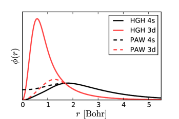
Figure 1: (Color online) The pseudo valence states of iron calculated with PAW and the norm-conserving HGH pseudopotentials. Both methods produce smooth wave functions for the delocalized 4s state, but the lack of norm conservation allows the short-ranged 3d state in PAW to be accurately sampled on a much coarser grid.

While LCAO pseudopotential codes as well as plane-wave/grid PAW codes already exist and have been discussed extensively in the literature,Sankey:1989 ; siesta ; Blochl:1994 the combination of LCAO and PAW is new. Compared to the popular Siesta method, which is based on norm-conserving pseudopotentials, the advantage of the present scheme (apart from the “double basis” feature) is that PAW works with coarser grids to represent the density and effective potentials. As an example, Fig. 1 shows the atomic orbitals of iron calculated with the norm-conserving Hartwigsen-Goedecker-Hutter (HGH) pseudopotentialshgh as well as with PAW. Clearly the $d$ wavefunction is much smoother in PAW. This is essential for larger systems where operations on the grid, i.e. solving the Poisson equation, evaluating the density, and calculating the potential matrix elements, become computationally demanding.

II Projector Augmented Wave Method

In this section we give a brief review of the PAW formalism. For simplicity we restrict the equations to the case of spin-paired, finite systems, but the generalizations to magnetic and periodic systems are straightforward. For a more comprehensive presentation we refer to Ref. Blochl:1994, .

II.1 PAW Transformation Operator

The PAW method is based on a linear transformation $\mathcal{T}$ which maps some computationally convenient “pseudo” or “smooth” wavefunctions $|\tilde{\psi}_{n}\rangle$ to the physically relevant “all-electron” wavefunctions $|\psi_{n}\rangle$:

$$|\psi_{n}\rangle=\mathcal{T}|\tilde{\psi}_{n}\rangle,$$ (1)

where $n$ is a quantum state label, consisting of a band index and possibly a spin and $\bm{\mathrm{k}}$-vector index.

The transformation is chosen as $\mathcal{T}=1+\sum_{a}\mathcal{T}^{a}$, i.e. the identity operator plus an additive contribution centered around each atom, which differs based on the species of atom.

The atomic contribution for atom $a$ is determined by choosing a set of smooth functions $\tilde{\phi}_{i}^{a}(\bm{\mathrm{r}})$, called pseudo partial waves, and requiring the transformation to map those onto the atomic valence orbitals $\phi_{i}^{a}(\bm{\mathrm{r}})$ of that atom, called all-electron partial waves. This effectively allows the all-electron behaviour to be incorporated by the smooth pseudo wave functions. Since the all-electron wave functions are smooth sufficiently far from the atoms, we may require the pseudo partial waves to match the all-electron ones outside a certain cutoff radius, such that $\tilde{\phi}_{i}^{a}(\bm{\mathrm{r}})=\phi_{i}^{a}(\bm{\mathrm{r}})$ for $r>r_{c}$. This localizes the atomic contribution $\mathcal{T}^{a}$ to the augmentation sphere $r<r_{c}$. Finally a set of localized projectors $\tilde{p}_{i}^{a}(\bm{\mathrm{r}})$ is chosen as a dual basis to the pseudo partial waves. We further want the partial wave-projector basis to be complete within the augmentation sphere, in the sense that any pseudo wave function should be expressible in terms of pseudo partial waves, and therefore require

$$\sum_{i}|\tilde{\phi}_{i}^{a}\rangle\langle\tilde{p}_{i}^{a}|=1,\qquad\langle\tilde{\phi}_{i}^{a}|\tilde{p}_{j}^{a}\rangle=\delta_{ij}.$$ (2)

The transformation $\mathcal{T}$ is then defined by

$$\mathcal{T}=1+\sum_{a}\sum_{i}(|\phi_{i}^{a}\rangle-|\tilde{\phi}_{i}^{a}\rangle)\langle\tilde{p}_{i}^{a}|,$$ (3)

which allows the all-electron Kohn-Sham wavefunction $\psi_{n}(\bm{\mathrm{r}})=\langle\bm{\mathrm{r}}|\psi_{n}\rangle$ to be recovered from a pseudo wave function through

$$\psi_{n}(\mathbf{r})=\tilde{\psi}_{n}(\mathbf{r})+\sum_{a}\sum_{i}(\phi_{i}^{a}(\mathbf{r})-\tilde{\phi}_{i}^{a}(\mathbf{r}))\langle\tilde{p}_{i}^{a}|\tilde{\psi}_{n}\rangle.$$ (4)

We emphasize that the all-electron wave functions are never evaluated explicitly, but all-electron values of observables are calculated through manipulations which rely only on coarse grids or one-dimensional radial grids. Using using Eqs. (1) and (3), the all-electron expectation value for any semi-local operator $O$ due to the valence states can be written

$$\langle O\rangle =\sum_{n}f_{n}\langle\tilde{\psi}_{n}|O|\tilde{\psi}_{n}\rangle$$

$$\quad+\sum_{naij}f_{n}\langle\tilde{\psi}_{n}|\tilde{p}_{i}^{a}\rangle\langle\phi_{i}^{a}|O|\phi_{j}^{a}\rangle\langle\tilde{p}_{j}^{a}|\tilde{\psi}_{n}\rangle$$

$$\quad-\sum_{naij}f_{n}\langle\tilde{\psi}_{n}|\tilde{p}_{i}^{a}\rangle\langle\tilde{\phi}_{i}^{a}|O|\tilde{\phi}_{j}^{a}\rangle\langle\tilde{p}_{j}^{a}|\tilde{\psi}_{n}\rangle.$$ (5)

Inside the augmentation spheres the partial wave expansion is ideally complete, so the first and third terms will cancel and leave only the all-electron contribution. Outside the augmentation spheres the pseudo partial waves are identical to the all-electron ones, so the two atomic terms cancel. The atomic matrix elements of $O$ in the second and third terms can be pre-evaluated for the isolated atom on high-resolution radial grids, so operations on smooth quantities, like $\langle\tilde{\psi}_{n}|O|\tilde{\psi}_{n}\rangle$ and $\langle\tilde{p}_{i}^{a}|\tilde{\psi}_{n}\rangle$, are the only ones performed during actual calculations.

It is convenient to define the atomic density matrices

$$D_{ij}^{a}=\sum_{n}\langle\tilde{p}_{i}^{a}|\tilde{\psi}_{n}\rangle f_{n}\langle\tilde{\psi}_{n}|\tilde{p}_{j}^{a}\rangle,$$ (6)

since these completely describe the dependence of the atomic terms in Eq. (5) on the pseudo wave functions. The expectation value can then be written

$$\langle O\rangle =\sum_{n}f_{n}\langle\tilde{\psi}_{n}|O|\tilde{\psi}_{n}\rangle$$

$$\quad+\sum_{aij}D_{ji}^{a}\left(\langle\phi_{i}^{a}|O|\phi_{j}^{a}\rangle-\langle\tilde{\phi}_{i}^{a}|O|\tilde{\phi}_{j}^{a}\rangle\right).$$ (7)

Although the PAW method is an exact implementation of density functional theory, some approximations are needed for realistic calculations. The frozen-core approximation assumes that the core states are localized within the augmentation spheres and that they are not modified by the chemical environment and hence taken from atomic reference calculations. The non-completeness of the basis, or equivalently the finite grid-spacing, will introduce an error in the evaluation of the PS contribution $\tilde{\psi}_{n}$ in (5). Finally, the number of partial waves and projector functions is obviously finite. This means that the completeness conditions of Eq. (2) we have required are not strictly fulfilled. This approximation can be controlled directly by increasing the number of partial waves and projectors.

II.2 Density

The electron density $n(\bm{\mathrm{r}})$ is the expectation value of the real-space projection operator and, by Eq. (7), takes the form

$$n(\bm{\mathrm{r}})=\tilde{n}(\bm{\mathrm{r}})+\sum_{a}\left[n^{a}(\bm{\mathrm{r}}-\bm{\mathrm{R}}^{a})-\tilde{n}^{a}(\bm{\mathrm{r}}-\bm{\mathrm{R}}^{a})\right],$$ (8)

where

$$\tilde{n}(\bm{\mathrm{r}}) =\sum_{n}f_{n}|\tilde{\psi}_{n}(\mathbf{r})|^{2}+\sum_{a}\tilde{n}_{c}^{a}(|\bm{\mathrm{r}}-\bm{\mathrm{R}}^{a}|),$$ (9)

$$n^{a}(\bm{\mathrm{r}}) =\sum_{ij}D_{ji}^{a}\phi_{i}^{a}(\bm{\mathrm{r}})\phi_{j}^{a}(\bm{\mathrm{r}})+n_{c}^{a}(r),$$ (10)

$$\tilde{n}^{a}(\bm{\mathrm{r}}) =\sum_{ij}D_{ji}^{a}\tilde{\phi}_{i}^{a}(\bm{\mathrm{r}})\tilde{\phi}_{j}^{a}(\bm{\mathrm{r}})+\tilde{n}_{c}^{a}(r).$$ (11)

Here we have separated out the all-electron core density $n_{c}^{a}(r)$ and the pseudo core density $\tilde{n}_{c}^{a}(r)$, where the latter can be chosen as any smooth continuation of $n_{c}^{a}(r)$ inside the augmentation spheres, since it will cancel out in Eq. (8). We omit conjugation of the partial waves since these can be chosen as real functions without loss of generality.

II.3 Compensation charges

In order to avoid dealing with the cumbersome nuclear point charges, and to compensate for the lack of norm-conservation, we introduce smooth localized compensation charges $\tilde{Z}^{a}(\bm{\mathrm{r}})$ on each atom, which are added to $\tilde{n}(\bm{\mathrm{r}})$ and $\tilde{n}^{a}(\bm{\mathrm{r}})$, thus keeping the total charge neutral. This yields a total charge density that can be expressed as

$$\rho(\bm{\mathrm{r}})=\tilde{\rho}(\bm{\mathrm{r}})+\sum_{a}\left[\rho^{a}(\bm{\mathrm{r}}-\bm{\mathrm{R}}^{a})-\tilde{\rho}^{a}(\bm{\mathrm{r}}-\bm{\mathrm{R}}^{a})\right],$$ (12)

in terms of the neutral charge densities

$$\tilde{\rho}(\bm{\mathrm{r}}) =\tilde{n}(\bm{\mathrm{r}})+\tilde{Z}(\bm{\mathrm{r}})=\tilde{n}(\bm{\mathrm{r}})+\sum_{a}\tilde{Z}^{a}(\bm{\mathrm{r}}-\bm{\mathrm{R}}^{a}),$$ (13)

$$\rho^{a}(\bm{\mathrm{r}}) =n^{a}(\bm{\mathrm{r}})+\mathcal{Z}^{a}\delta(\bm{\mathrm{r}}),$$ (14)

$$\tilde{\rho}^{a}(\bm{\mathrm{r}}) =\tilde{n}^{a}(\bm{\mathrm{r}})+\tilde{Z}^{a}(\bm{\mathrm{r}}),$$ (15)

where $\mathcal{Z}^{a}\delta(\bm{\mathrm{r}})$ is the central nuclear point charge. The compensation charges are chosen to be localized functions around each atom of the form

$$\tilde{Z}^{a}(\bm{\mathrm{r}})=\sum_{L}Q_{L}^{a}\tilde{g}_{L}^{a}(\bm{\mathrm{r}})=\sum_{lm}Q_{lm}^{a}r^{l}\tilde{g}_{l}^{a}(r)Y_{lm}(\hat{\bm{\mathrm{r}}}),$$ (16)

where $\tilde{g}_{l}^{a}(r)$ are fixed Gaussians, and $Y_{lm}(\hat{\bm{\mathrm{r}}})$ are spherical harmonics. We use $L=l,m$ as a composite index for angular and magnetic quantum numbers. The expansion coefficients $Q_{L}^{a}$ are determined in terms of $D_{ij}^{a}$ by requiring the compensation charges to cancel all the multipole moments of each augmentation region up to some order, generally $l_{\mathrm{max}}=2$. The charges will therefore dynamically adapt to the surroundings of the atom. For more details we refer to the original work by BlöchlBlochl:1994 .

II.4 Total Energy

The total energy can also be separated into smooth and atom-centered contributions

$$E=\tilde{E}+\sum_{a}(E^{a}-\tilde{E}^{a}),$$ (17)

where

$$\tilde{E} =\sum_{n}f_{n}\langle\tilde{\psi}_{n}|-\tfrac{1}{2}\nabla^{2}|\tilde{\psi}_{n}\rangle+\sum_{a}\int\tilde{n}(\bm{\mathrm{r}})\bar{v}^{a}(|\bm{\mathrm{r}}-\bm{\mathrm{R}}^{a}|)\,\mathrm{d}\bm{\mathrm{r}}$$

$$\quad+\frac{1}{2}\iint\frac{\tilde{\rho}(\mathbf{r})\tilde{\rho}(\mathbf{r^{\prime}})}{|\mathbf{r}-\mathbf{r^{\prime}}|}\,\mathrm{d}\bm{\mathrm{r}}\,\mathrm{d}\bm{\mathrm{r}}^{\prime}+E_{xc}[\tilde{n}],$$ (18)

$$E^{a} =\sum_{ij}D_{ji}^{a}\langle\phi^{a}_{i}|-\tfrac{1}{2}\nabla^{2}|\phi^{a}_{j}\rangle+T_{\mathrm{core}}^{a}$$

$$+\frac{1}{2}\iint\frac{\rho^{a}(\bm{\mathrm{r}})\rho^{a}(\bm{\mathrm{r}}^{\prime})}{|\bm{\mathrm{r}}-\bm{\mathrm{r}}^{\prime}|}\,\mathrm{d}\bm{\mathrm{r}}\,\mathrm{d}\bm{\mathrm{r}}^{\prime}+E_{xc}[n^{a}],$$ (19)

$$\tilde{E}^{a} =\sum_{ij}D_{ji}^{a}\langle\tilde{\phi}^{a}_{i}|-\tfrac{1}{2}\nabla^{2}|\tilde{\phi}^{a}_{j}\rangle+\tilde{T}_{\mathrm{core}}^{a}+\int\tilde{n}^{a}(\bm{\mathrm{r}})\bar{v}^{a}(r)\,\mathrm{d}\bm{\mathrm{r}}$$

$$+\frac{1}{2}\iint\frac{\tilde{\rho}^{a}(\mathbf{r})\tilde{\rho}^{a}(\mathbf{r^{\prime}})}{|\mathbf{r}-\mathbf{r^{\prime}}|}\,\mathrm{d}\bm{\mathrm{r}}\,\mathrm{d}\bm{\mathrm{r}}^{\prime}+E_{xc}[\tilde{n}^{a}].$$ (20)

The terms $T_{\mathrm{core}}^{a}$ and $\tilde{T}_{\mathrm{core}}^{a}$ are the kinetic energy contributions from the frozen core states, while $\bar{v}^{a}(r)$ is an arbitrary potential, vanishing for $r>r^{a}_{c}$. This potential is generally chosen to make the atomic potential smooth, while its contribution to the total energy vanishes if the partial wave expansion is complete.Mortensen:2005

$E_{\mathrm{xc}}$ is the exchange-correlation functional, which must be local or semilocal as per Eq. (7) for the above expressions to be correct. While the functional is non-linear, it remains true that

$$E_{\mathrm{xc}}[n]=E_{\mathrm{xc}}[\tilde{n}]+\sum_{a}\left(E_{\mathrm{xc}}[n^{a}]-E_{\mathrm{xc}}[\tilde{n}^{a}]\right),$$ (21)

because of the functional’s semilocality: the energy contribution from $\tilde{n}(\bm{\mathrm{r}})$ around every point inside the augmentation sphere is exactly cancelled by that of $\tilde{n}^{a}(\bm{\mathrm{r}})$, since $\tilde{n}(\bm{\mathrm{r}})$ and $\tilde{n}^{a}(\bm{\mathrm{r}})$ are exactly identical here, leaving only the contribution $E_{\mathrm{xc}}[n^{a}]$. Outside the augmentation region, a similar argument applies to $n^{a}(\bm{\mathrm{r}})$ and $\tilde{n}(\bm{\mathrm{r}})$, leaving only the energy contribution from $\tilde{n}(\bm{\mathrm{r}})$ which is here equal to the all-electron density.

II.5 Hamiltonian and orthogonality

In generic operator form, the Hamiltonian corresponding to the total energy from Eq. (17) is

$$\tilde{H}=-\tfrac{1}{2}\nabla^{2}+\tilde{v}+\sum_{aij}|\tilde{p}_{i}^{a}\rangle\Delta H_{ij}^{a}\langle p_{j}^{a}|,$$ (22)

where $\tilde{v}=\tilde{v}_{\mathrm{Ha}}[\tilde{\rho}]+\bar{v}+v_{\mathrm{xc}}[\tilde{n}]$ is the local effective potential, containing the Hartree, the arbitrary localized and the xc potentials, and where

$$\Delta H_{ij}^{a}=\frac{\partial E}{\partial D_{ji}^{a}}$$ (23)

are the atomic Hamiltonians containing the atom-centered contributions from the augmentation spheres. Since the all-electron wave functions $\psi_{n}$ must be orthonormal, the pseudo wave functions $\tilde{\psi}_{n}$ must obey

$$\delta_{nm}=\langle\psi_{n}|\psi_{m}\rangle=\langle\tilde{\psi}_{n}|\mathcal{T}^{\dagger}\mathcal{T}|\tilde{\psi}_{m}\rangle=\langle\tilde{\psi}_{n}|S|\tilde{\psi}_{m}\rangle,$$ (24)

where we have defined the overlap operator

$$S=\mathcal{T}^{\dagger}\mathcal{T}=1+\sum_{aij}|\tilde{p}_{i}^{a}\rangle\Delta S_{ij}^{a}\langle\tilde{p}_{j}^{a}|.$$ (25)

The atomic contributions

$$\Delta S_{ij}^{a}=\langle\phi_{i}^{a}|\phi_{j}^{a}\rangle-\langle\tilde{\phi}_{i}^{a}|\tilde{\phi}_{j}^{a}\rangle$$ (26)

are constant for a given element.

Given the Hamiltonian and orthogonality condition, a variational problem can be derived for the pseudo wave functions. This problem is equivalent to the generalized Kohn-Sham eigenvalue problem

$$\tilde{H}|\tilde{\psi}_{n}\rangle=S|\tilde{\psi}_{n}\rangle\epsilon_{n},$$ (27)

which can then be solved self-consistently with available techniques.

III Localized basis sets in PAW

We now introduce a set of basis functions $|\Phi_{\mu}\rangle$ which are fixed, strictly localized atomic orbital-like functions represented numerically, following the approach by Sankey and NiklewskiSankey:1989 . We furthermore consider the pseudo wave functions $|\tilde{\psi}_{n}\rangle$ to be linear combinations of the new basis functions

$$|\tilde{\psi}_{n}\rangle=\sum_{\mu}c_{\mu n}|\Phi_{\mu}\rangle,$$ (28)

where the coefficients $c_{\mu n}$ are variational parameters. It proves useful to define the density matrix

$$\rho_{\mu\nu}=\sum_{n}c_{\mu n}f_{n}c_{\nu n}^{*}.$$ (29)

The pseudo density can be evaluated from the density matrix through

$$\tilde{n}(\bm{\mathrm{r}})=\sum_{\mu\nu}\Phi_{\mu}^{*}(\bm{\mathrm{r}})\Phi_{\nu}(\bm{\mathrm{r}})\rho_{\nu\mu}+\sum_{a}\tilde{n}_{c}^{a}(\bm{\mathrm{r}}).$$ (30)

Ahead of a calculation, we evaluate the matrices

$$T_{\mu\nu} =\langle\Phi_{\mu}|-\tfrac{1}{2}\nabla^{2}|\Phi_{\nu}\rangle,$$ (31)

$$P_{i\mu}^{a} =\langle\tilde{p}_{i}^{a}|\Phi_{\mu}\rangle,$$ (32)

$$\Theta_{\mu\nu} =\langle\Phi_{\mu}|\Phi_{\nu}\rangle,$$ (33)

which are used to evaluate most of the quantities of the previous sections in matrix form. The atomic density matrices from Eq. (6) become

$$D_{ij}^{a}=\sum_{\mu\nu}P_{i\mu}^{a}\rho_{\mu\nu}P_{j\nu}^{a*},$$ (34)

and the kinetic energy contribution in the first term of Eq. (18) is

$$\sum_{n}f_{n}\langle\tilde{\psi}_{n}|-\tfrac{1}{2}\nabla^{2}|\tilde{\psi}_{n}\rangle=\sum_{\mu\nu}T_{\mu\nu}\rho_{\nu\mu}.$$ (35)

We can then define the Hamiltonian matrix elements by taking the derivative of the total energy $E$ with respect to the density matrix elements, which eventually results in the discretized Hamiltonian

$$H_{\mu\nu}\equiv\frac{\partial E}{\partial\rho_{\nu\mu}}=T_{\mu\nu}+V_{\mu\nu}+\sum_{aij}P_{i\mu}^{a*}\Delta H_{ij}^{a}P_{j\nu}^{a},$$ (36)

where

$$V_{\mu\nu}=\int\Phi_{\mu}^{*}(\bm{\mathrm{r}})\tilde{v}(\bm{\mathrm{r}})\Phi_{\nu}(\bm{\mathrm{r}})\,\mathrm{d}\bm{\mathrm{r}}.$$ (37)

The overlap operator of Eq. (25) has the matrix representation

$$S_{\mu\nu}=\langle\Phi_{\mu}|S|\Phi_{\nu}\rangle=\Theta_{\mu\nu}+\sum_{aij}P_{i\mu}^{a*}\Delta S_{ij}^{a}P_{j\nu}^{a},$$ (38)

so orthogonality of the wave functions is now expressed by

$$\sum_{\mu\nu}c_{\mu m}^{*}S_{\mu\nu}c_{\nu n}=\delta_{mn}.$$ (39)

This is incorporated by defining a quantity $\Omega$ to be variationally minimized with respect to the coefficients, specifically

$$\Omega=E-\sum_{mn\mu\nu}\lambda_{nm}\left(c_{\mu m}^{*}S_{\mu\nu}c_{\nu n}-\delta_{mn}\right).$$ (40)

Setting the derivative of $\Omega$ with respect to $c_{\mu n}$ equal to 0, one obtains the generalized eigenvalue equation

$$\sum_{\nu}H_{\mu\nu}c_{\nu n}=\sum_{\nu}S_{\mu\nu}c_{\nu n}\epsilon_{n},$$ (41)

which can be solved for the coefficients $c_{\mu n}$ and energies $\epsilon_{n}$ when the Hamiltonian $H_{\mu\nu}$ and the overlap matrix $S_{\mu\nu}$ are known.

III.1 Basis functions generation

The basis functions $|\Phi_{\mu}\rangle$ in Eq. (28) are atom-centered orbitals written as products of numerical radial functions and spherical harmonics:

$$\Phi_{nlm}(\bm{\mathrm{r}})=\varphi_{nl}(r)Y_{lm}(\hat{\bm{\mathrm{r}}}).$$ (42)

In order to make the Hamiltonian and overlap matrices sparse in the basis-set representation, we use strictly localized radial functions, i.e. orbitals that are identically zero beyond a given radius, as proposed by Sankey and Niklewski Sankey:1989 and successfully implemented in the SIESTA method siesta .

The first (single-zeta) basis orbitals $\varphi_{nl}^{\mathrm{AE}}(r)$ are obtained for each valence state by solving the radial all-electron Kohn-Sham equations for the isolated atom in the presence of a confining potential with a certain cutoff. If the confining potential is chosen to be smooth, the basis functions similarly become smooth. We use the same confining potential as proposed in Ref. siesta2, . The smooth basis functions are then obtained using $\varphi_{nl}(r)=\mathcal{T}^{-1}\varphi_{nl}^{\mathrm{AE}}(r)$. The result of the procedure is illustrated in Fig. 2.

The cutoff radius is selected in a systematic way by specifying the energy shift $\Delta E$ of the confined orbital compared to the free-atom orbital. In this approach small values of $\Delta E$ will correspond to long-ranged basis orbitalssiesta .

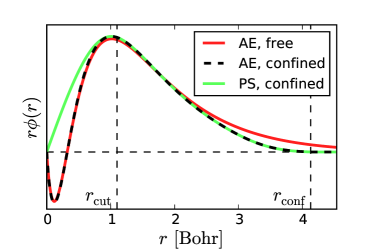
Figure 2: NAO generation for the nitrogen 2s state: the all-electron orbital of the free atom, the confined all-electron orbital, and the corresponding pseudo wave function after applying the inverse PAW transformation. The augmentation sphere and basis function cutoffs are indicated.

To improve the radial flexibility, extra basis functions with the same angular momentum $l$ (multiple-zeta) are constructed for each valence state using the split-valence techniquesiesta . The extra function is constructed by matching a polynomial to the tail of the atomic orbital, where the matching radius is determined by requiring the norm of the part of the atomic orbital outside that radius to have a certain value.

Finally, polarization functions (basis functions with $l$ quantum number corresponding to the lowest unoccupied angular momentum) can be added in order to improve the angular flexibility of the basis. There are several approaches to generate these orbitals, such as perturbing the occupied eigenstate with the highest $l$ quantum number with an electric field using first order perturbation theory (like in Ref. siesta, ) or using the appropriate unoccupied orbitals. As a first implementation we use a Gaussian-like function of the form $r^{l}\exp(-\alpha r^{2})$ for the radial part, where $l$ corresponds to the lowest unoccupied angular momentum. This produces reasonable polarization functions as demonstrated by the results presented in a following section.

A generator program is included in the GPAW code and it can produce basis sets for virtually any elements in the periodic table. Through our experiences with generating and using different basis sets, we have reached the following set of default parameters: We usually work with a DZP basis. The energy shift for the atomic orbital is taken as 0.1 eV, and the tail-norm is 0.16 (in agreement with SIESTAsiesta ). The width of the Gaussian used for the polarization function is 1/4 of the cut-off radius of the first zeta basis function. Further information can be found in the documentation for the basis set generator. At this point we have not yet systematically optimized the basis set parameters, although we expect to do so by means of an automatic procedure.

III.2 Atomic forces

The force on some atom $a$ is defined as the negative derivative of the total energy of the system with respect to the position of that atom,

$$\bm{\mathrm{F}}^{a}=-\frac{\partial E}{\partial\bm{\mathrm{R}}^{a}}.$$ (43)

The derivative is to be taken with the constraints that selfconsistency and orthonormality according to (39) must be obeyed. This implies that the calculated force will correspond to the small-displacement limit of the finite-difference energy gradient one would obtain by performing two separate energy calculations, where atom $a$ is slightly displaced in one of them.

The expression for the force is obtained by using the chain rule on the total energy of Eq. (17). The primary complication compared to the grid-based PAW force formula, Eq. (50) from Ref. Mortensen:2005, , is that the basis functions move with the atoms, introducing extra terms in the derivative.

The complete formula for the force on atom $a$ is

$$\bm{\mathrm{F}}^{a} =2\Re\sum_{\mu\in a;\nu}\frac{\mathrm{d}T_{\mu\nu}}{\mathrm{d}\bm{\mathrm{R}}^{a}}\rho_{\nu\mu}-2\Re\sum_{\mu\in a;\nu}\frac{\mathrm{d}\Theta_{\mu\nu}}{\mathrm{d}\bm{\mathrm{R}}^{a}}E_{\nu\mu}$$

$$+2\Re\sum_{b;\mu\in a;\nu}\bm{\mathrm{Z}}_{\mu\nu}^{b}E_{\nu\mu}-2\Re\sum_{\mu\nu}\bm{\mathrm{Z}}_{\mu\nu}^{a}E_{\nu\mu}$$

$$-2\Re\sum_{b;\nu;\mu\in a}\bm{\mathrm{A}}_{\mu\nu}^{b}\rho_{\nu\mu}+2\Re\sum_{\mu\nu}\bm{\mathrm{A}}_{\mu\nu}^{a}\rho_{\nu\mu}$$

$$+2\Re\sum_{\mu\in a;\nu}\left[\int\frac{\mathrm{d}\Phi_{\mu}^{*}(\bm{\mathrm{r}})}{\mathrm{d}\bm{\mathrm{R}}^{a}}\tilde{v}(\bm{\mathrm{r}})\Phi_{\nu}(\bm{\mathrm{r}})\,\mathrm{d}\bm{\mathrm{r}}\right]\rho_{\nu\mu}$$

$$-\int\tilde{v}(\bm{\mathrm{r}})\frac{\mathrm{d}\tilde{n}_{c}^{a}(|\bm{\mathrm{r}}-\bm{\mathrm{R}}^{a}|)}{\mathrm{d}\bm{\mathrm{R}}^{a}}\,\mathrm{d}\bm{\mathrm{r}}-\int\tilde{n}(\bm{\mathrm{r}})\frac{\mathrm{d}\bar{v}^{a}(|\bm{\mathrm{r}}-\bm{\mathrm{R}}^{a}|)}{\mathrm{d}\bm{\mathrm{R}}^{a}}\,\mathrm{d}\bm{\mathrm{r}}$$

$$-\int\tilde{v}_{H}(\bm{\mathrm{r}})\sum_{L}Q_{L}^{a}\frac{\mathrm{d}\tilde{g}_{L}^{a}(\bm{\mathrm{r}}-\bm{\mathrm{R}}^{a})}{\mathrm{d}\bm{\mathrm{R}}^{a}}\,\mathrm{d}\bm{\mathrm{r}},$$ (44)

where

$$\bm{\mathrm{A}}_{\mu\nu}^{b} =\sum_{ij}\frac{\mathrm{d}P_{i\mu}^{b*}}{\mathrm{d}\bm{\mathrm{R}}^{a}}\Delta H_{ij}^{b}P_{j\nu}^{b},$$ (45)

$$\bm{\mathrm{Z}}_{\mu\nu}^{b} =\sum_{ij}\frac{\mathrm{d}P_{i\mu}^{b*}}{\mathrm{d}\bm{\mathrm{R}}^{a}}\Delta S_{ij}^{b}P_{j\nu}^{b},$$ (46)

$$E_{\mu\nu} =\sum_{\lambda\xi}S^{-1}_{\mu\lambda}H_{\lambda\xi}\rho_{\xi\nu}.$$ (47)

The notation $\mu\in a$ denotes that summation should be performed only over those basis functions that reside on atom $a$.

Eq. (44) is derived in Appendix A. The last three terms are basis set independent, and inherited from the grid-based implementation.

IV Implementation

The LCAO code is implemented in GPAW, a real-space PAW code. For the details of the real-space implementation we refer to the original paperMortensen:2005 . In this code the density, effective potential and wave functions are evaluated on real-space grids.

In LCAO the matrix elements of the kinetic and overlap operators $T_{\mu\nu}$, $\Theta_{\mu\nu}$ and $P_{i\mu}^{a}$ in Eqs. (31)-(33) are efficiently calculated in Fourier space based on analytical expressionsSankey:1989 . For each pair of different basis orbitals (i.e. independently of the atomic positions), the overlap can be represented in the form of radial functions and spherical harmonics. These functions are stored as splines which can in turn be evaluated for a multitude of different atomic separations.

The two-center integrals are thus calculated once for a given atomic configuration ahead of the self-consistency loop. This is equivalent to the SIESTA approachsiesta .

The matrix elements of the effective potential $V_{\mu\nu}$ are still calculated numerically on the three dimensional real-space grid, since the density is also evaluated on this gridMortensen:2005 .

Because of the reduced degrees of freedom of a basis calculation compared to a grid-based calculation, the Hamiltonian from Eq. (36) is directly diagonalized in the space of the basis functions according to Eq. (41). This considerably lowers the number of required iterations to reach selfconsistency, compared to the iterative minimization schemes used in grid-based calculations.

For each step in the selfconsistency loop, the Hartree potential $\tilde{v}_{\mathrm{Ha}}(\bm{\mathrm{r}})$ is calculated by solving the Poisson equation $\nabla^{2}\tilde{v}_{\mathrm{Ha}}(\bm{\mathrm{r}})=-4\pi\tilde{\rho}(\bm{\mathrm{r}})$ in real space using existing multigrid methods, such as the Gauss-Seidel and Jacobi methods. A solver based on the fast Fourier transform is also available in the GPAW code.

The calculations are parallelized over k-points, spins and real-space domains like in the grid-based caseMortensen:2005 . We further distribute the orbital-by-orbital matrices such as $H_{\mu\nu}$ and $S_{\mu\nu}$, and use ScaLAPACK for operations on these, notably the diagonalization of Eq. (41).

IV.1 Localized functions on the grid

Quantities such as the density $\tilde{n}(\bm{\mathrm{r}})$ and effective potential $\tilde{v}(\bm{\mathrm{r}})$ are still stored on 3D grids. Matrix elements like $V_{\mu\nu}$ in Eq. (37), and the pseudo density given by Eq. (30), can therefore be calculated by loops over grid points.

Since each basis function is nonzero only in a small part of space, we only store the values of a given function within its bounding sphere. Each function value inside the bounding sphere is calculated as the product of radial and angular parts vz. Eq. (42), where the radial part is represented by a spline, and the spherical harmonic evaluated in cartesian form, i.e. as a polynomial. The same method is used to evaluate derivatives in force calculations, although this involves the derivatives of these quantities aside from just their function values.

We initially compile a data structure to keep track of which functions are nonzero for each grid point. When looping over the grid, we maintain a list of indices $\mu$ for the currently nonzero functions by adding or removing, as appropriate, those functions whose bounding spheres we intersect. The locations of these bounding spheres are likewise precompiled into lists for efficient processing. The memory overhead due to this method is still much smaller than the storage requirements for the actual function values.

V Results

In this section we calculate common quantities using the localized basis set on different systems. The results are compared to the complete basis set limit, i.e. a well converged grid calculation. Note that this comparison can be done in a very systematic way since the calculations on the grid share the same approximations and mostly the same implementation as the calculations performed with the localized basis. All the results presented in this section have been obtained using PAW setups from the extensive GPAW library, freely available onlinesetups .

V.1 Molecules

In order to assess the accuracy of the LCAO implementation for small molecules, the PBEpbe atomization energies for the G2-1 data-setCurtiss:1997 are considered. The atomic coordinates are taken from MP2(full)/6-31G(d) optimized geometries. The error with respect to the grid results is shown in Fig. 3 for different basis sets. This error is defined as

$$\Delta E^{\mathrm{LCAO}}-\Delta E^{\mathrm{grid}} =E^{\mathrm{LCAO}}_{\mathrm{mol}}-\sum_{\mathrm{atoms}}E^{\mathrm{LCAO}}_{\mathrm{atoms}}$$

$$\quad-\left(E^{\mathrm{grid}}_{\mathrm{mol}}-\sum_{\mathrm{atoms}}E^{\mathrm{grid}}_{\mathrm{atoms}}\right)$$ (48)

The reference grid results are well converged calculations in very good agreement with the VASPvasp and Gaussiangaussian codes.

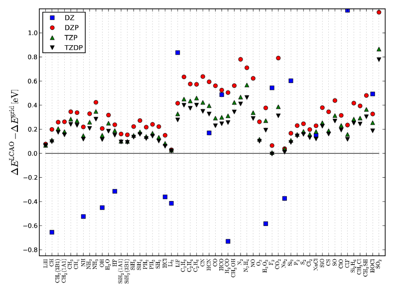
Figure 3: (Color online) PBE atomization energies from the G2-1 dataset, relative to the grid values. The corresponding Mean Absolute Errors with respect to the grid values are: 1.71 eV (20.4%) for Double Zeta (DZ); 0.36eV (4.45%) for Double Zeta Polarized (DZP); 0.25 eV (3.02%) for Triple Zeta Polarized (TZP)and 0.20 eV (2.44%) for Triple Zeta Double Polarized (TZDP).

The figure shows that enlarging the basis set, i.e. including more orbitals per valence electron, systematically improves the results towards the grid energies.

It must be noted that some differences with respect to the grid atomization energies still remain, even in the case of large basis sets. This is mainly due to the two following reasons. Firstly, the basis functions are generated from spin-paired calculations and hence they do not explicitly account for possible spin-polarized orbitals. This is in practice accounted for by using larger basis-sets in order to include more degrees of freedom in the shape of the wavefunctions. Secondly, isolated atoms are difficult to treat because of their long ranged orbitals. Actual basis functions are, in fact, obtained from atomic calculations with an artificial confining potential thus resulting in more confined orbitals.

V.2 Solids

The equilibrium bulk properties have been calculated for several crystals featuring different electronic structures: simple metals (Li, Na, Al), semiconductors (AlP, Si, SiC), ionic solids (NaCl, LiF, MgO) transition metals (Fe, Cu, Pt) as well as one insulator (C). The results are shown in Fig. 4. For comparison with grid-based calculations, the bar plots show the deviations from grid-based results for each basis set, while the precise numbers are shown in each of the corresponding tables. All the calculations were performed with the solids in their lowest energy crystal structure, using the PBE functional for exchange and correlationpbe . The quantities were computed using the relaxed structures obtained with the default, unoptimized basis sets. The calculations were generally spin-paired, i.e. non-magnetic, with the exception of Fe and the atomic calculations used to get cohesive energies.

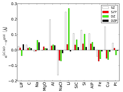
	$a$ (Å)
	SZ	SZP	DZ	DZP	GRID
LiF	4.08	4.08	4.02	4.10	4.06
C	3.61	3.58	3.59	3.58	3.57
Na	4.18	4.19	4.26	4.24	4.19
MgO	4.26	4.28	4.27	4.27	4.26
Al	4.24	4.07	4.08	4.07	4.04
NaCl	5.52	5.62	5.61	5.67	5.69
Li	3.68	3.47	3.70	3.43	3.43
SiC	4.50	4.42	4.46	4.41	4.39
Si	5.60	5.52	5.58	5.49	5.48
AlP	5.62	5.55	5.56	5.53	5.51
Fe	2.80	2.77	2.78	2.83	2.84
Cu	3.80	3.59	3.58	3.64	3.65
Pt	4.02	3.99	3.95	3.98	3.98
MAE	0.097	0.034	0.068	0.019
MAE %	2.33	0.84	1.70	0.45

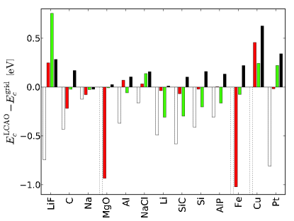
	$E_{c}$ (eV)
	SZ	SZP	DZ	DZP	GRID
LiF	3.49	4.48	4.99	4.52	4.24
C	7.29	7.51	7.70	7.89	7.72
Na	0.97	1.02	1.07	1.07	1.09
MgO	2.81	4.01	4.94	4.97	4.95
Al	3.07	3.51	3.38	3.54	3.43
NaCl	2.94	3.14	3.24	3.26	3.10
Li	1.13	1.58	1.31	1.63	1.62
SiC	5.80	6.31	6.08	6.48	6.38
Si	4.14	4.52	4.34	4.71	4.55
AlP	3.77	4.09	3.92	4.21	4.08
Fe	1.34	3.83	4.77	5.07	4.85
Cu	2.38	3.97	3.75	4.14	3.51
Pt	4.54	5.33	5.57	5.69	5.35
MAE	0.86	0.25	0.19	0.18
MAE %	20.70	5.86	5.51	4.40

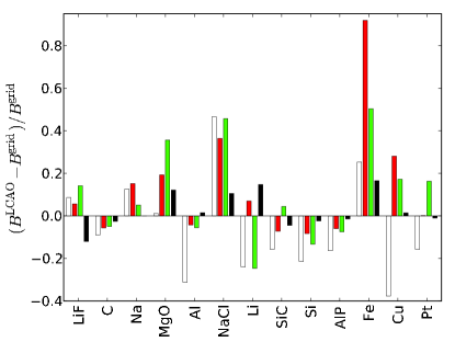
	$B$ (GPa)
	SZ	SZP	DZ	DZP	GRID
LiF	87	84	91	70	80
C	394	408	411	422	433
Na	8.9	9.1	8.3	7.9	7.9
MgO	156	184	209	173	154
Al	53	74	73	79	77
NaCl	35	32	34	26	24
Li	10.8	15.2	10.7	16.3	14.2
SiC	178	196	221	202	211
Si	70	81	77	86	88
AlP	69	77	76	81	82
Fe	248	379	297	231	198
Cu	88	181	166	143	141
Pt	224	266	309	263	266
MAE	22.9	24.8	23.2	7.4
MAE %	20.4	18.2	18.8	6.3

Figure 4: (Color online) Deviations in cohesive energy (top), lattice parameter (middle) and relative bulk modulus (bottom) from the converged grid results. The largest bars have been truncated and are shown with dotted edges – see the corresponding tables for the precise values.

The overall agreement with the real-space grid is excellent: about 0.5% mean absolute error in the computation of lattice constants, 4% in cohesive energies and 5-8% for bulk moduli using DZP basis sets. Notice that in many cases remarkably good results can be obtained even with a small SZP basis, particularly for lattice constants. This shows that structure optimizations with the LCAO code are likely to yield very accurate geometries. This is probably due to the fact that calculations of equilibrium structures only involve energy differences between very similar structures, i.e. not with respect to isolated atoms, thus leading to larger error cancellations.

With DZP the primary source of error in cohesive energy comes from the free-atom calculation, where the confinement of each orbital raises the energy levels by around 0.1 eV. Thus, atomic energies are systematically overestimated, leading to stronger binding. This error can be controlled by using larger basis set cutoffs, i.e. choosing smaller orbital energy shifts during basis generation.

V.3 Structure optimizations

LCAO calculations tend to reproduce geometries of grid-based calculations very accurately. In structure optimizations, the LCAO code can therefore be used to provide a high-quality initial guess for a grid-based structure optimization.

While it is trivial to reuse a geometry obtained in one code for a more accurate optimization in another, our approach is practical because the two representations share the exact same framework. Thus the procedure is seamless as well as numerically consistent, in the sense that most of the operations are carried out using the same approximations, finite-difference stencils and so on. With quasi-Newton methods, the estimate of the Hessian matrix generated during the LCAO optimization can be reused as well. For most non-trivial systems, an LCAO calculation is between 25 and 30 times faster than a grid calculation, making the cost of the LCAO optimization negligible.

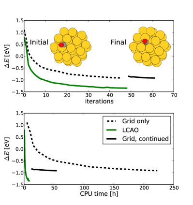
Figure 5: (Color online) The energy as a function of iteration count (top) as well as CPU time (bottom) in structure optimizations. Shows a grid-based and an LCAO based structure optimization plus the continuation of the LCAO optimization after switching to the grid representation.

Fig. 5 shows a performance comparison when reusing the positions and Hessian from a LCAO-based structure optimization for a grid-based one, using the default basis set. The system is a 38-atom truncated octahedral gold cluster with CO adsorbed, with the initial and final geometries shown in the inset.

A purely grid-based optimization takes 223 CPU hours while a purely LCAO-based one, requiring roughly the same number of steps, takes 8.4 CPU hours. A further grid-based optimization takes 45 CPU hours, for a total speedup factor of 4. The value of an initial LCAO optimization is of course higher if the initial guess is worse. For systems where a large fraction of the time is spent close to the converged geometry, the speedup may not be as significant.

The energy reference corresponds to the separate cluster and molecule at optimized geometries – the total energy difference between an LCAO and a grid calculation is otherwise around 30 eV. It is therefore important to choose an optimization algorithm which will handle such a shift well. The present plots use the L-BFGS algorithmsheppard ; nocedal (limited memory Broyden-Fletcher-Goldfarb-Shanno) from the Atomic Simulation Environment.ase

VI Conclusions

We have described the implementation of a localized basis in the grid based PAW code GPAW, and tested the method on a variety of molecules and solids. The results for atomization energies, cohesive energies, lattice parameters and bulk moduli were shown to converge towards the grid results as the size of the LCAO basis was increased. Structural properties were found to be particularly accurate with the LCAO basis. It has been demonstrated how the LCAO basis can be used to produce accurate initial guesses (both for the electron wavefunctions, atomic structure, and Hessian matrix) for subsequent grid-based calculations to increase efficiency of high-accuracy grid calculations.

The combination of the grid-based and LCAO methods in one code provides a flexible, simple and smooth way to switch between the two representations. Furthermore the PAW formalism itself presents significant advantages: it is an all-electron method, which eliminates pseudopotential errors, and it allows the use of coarser grids than norm-conserving pseudopotentials, which increases efficiency.

Finally, the LCAO method enables GPAW to perform calculations involving Green’s function, which intrinsically need a basis set with finite support. Current developments along these lines include electron transport calculations, electron-phonon coupling and STM simulations.

Appendix A Force formula

The force on atom $a$ is found by taking the derivative of the total energy with respect to the atomic position $\bm{\mathrm{R}}^{a}$. We shall use the chain rule on Eq. (17), taking $\rho_{\mu\nu}$, $D_{ij}^{a}$, $\tilde{n}(\bm{\mathrm{r}})$, $\tilde{\rho}(\bm{\mathrm{r}})$, $T_{\mu\nu}$ and $\bar{v}(\bm{\mathrm{r}})$ to be separate variables for the purposes of partial derivatives:

$$\frac{\partial E}{\partial\bm{\mathrm{R}}^{a}} =\sum_{\mu\nu}\frac{\partial E}{\partial\rho_{\nu\mu}}\frac{\partial\rho_{\nu\mu}}{\partial\bm{\mathrm{R}}^{a}}+\sum_{bij}\frac{\partial E}{\partial D_{ji}^{b}}\frac{\partial D_{ji}^{b}}{\partial\bm{\mathrm{R}}^{a}}$$

$$\quad+\int\frac{\delta E}{\delta\tilde{n}(\bm{\mathrm{r}})}\frac{\partial\tilde{n}(\bm{\mathrm{r}})}{\partial\bm{\mathrm{R}}^{a}}\,\mathrm{d}\bm{\mathrm{r}}+\int\frac{\delta E}{\delta\tilde{\rho}(\bm{\mathrm{r}})}\frac{\partial\tilde{\rho}(\bm{\mathrm{r}})}{\partial\bm{\mathrm{R}}^{a}}\,\mathrm{d}\bm{\mathrm{r}}$$

$$\quad+\sum_{\mu\nu}\frac{\partial E}{\partial T_{\mu\nu}}\frac{\partial T_{\mu\nu}}{\partial\bm{\mathrm{R}}^{a}}+\int\frac{\delta E}{\delta\bar{v}(\bm{\mathrm{r}})}\frac{\partial\bar{v}(\bm{\mathrm{r}})}{\partial\bm{\mathrm{R}}^{a}}\,\mathrm{d}\bm{\mathrm{r}},$$ (49)

where $\bar{v}(\bm{\mathrm{r}})=\sum_{a}\bar{v}^{a}(|\bm{\mathrm{r}}-\bm{\mathrm{R}}^{a}|)$. The remaining quantities in the energy expression pertain to isolated atoms, and thus do not depend on atomic positions. The first term of Eq. (49) is

$$\sum_{\mu\nu}\frac{\partial E}{\partial\rho_{\nu\mu}}\frac{\partial\rho_{\nu\mu}}{\partial\bm{\mathrm{R}}^{a}} =2\Re\sum_{\mu\nu n}H_{\mu\nu}c_{\nu n}f_{n}\frac{\partial c_{\mu n}^{*}}{\partial\bm{\mathrm{R}}^{a}}$$

$$=2\Re\sum_{\mu\nu n}\frac{\partial c_{\mu n}^{*}}{\partial\bm{\mathrm{R}}^{a}}S_{\mu\nu}c_{\nu n}\epsilon_{n}f_{n},$$ (50)

where we have used Eqs. (29) and (36) in the first step, and Eq. (41) in the second. When the atoms are displaced (infinitesimally), the coefficients must change to accommodate the orthogonality criterion. This can be incorporated by requiring the derivatives of each side of Eq. (39) to be equal, implying the relationship

$$-\sum_{\mu\nu}c_{\mu n}^{*}\frac{\partial S_{\mu\nu}}{\partial\bm{\mathrm{R}}^{a}}c_{\nu n}=2\Re\sum_{\mu\nu}\frac{\partial c_{\mu n}^{*}}{\partial\bm{\mathrm{R}}^{a}}S_{\mu\nu}c_{\nu n}.$$ (51)

Inserting this into Eq. (50) yields

$$\sum_{\mu\nu}\frac{\partial E}{\partial\rho_{\nu\mu}}\frac{\partial\rho_{\nu\mu}}{\partial\bm{\mathrm{R}}^{a}} =-\sum_{\mu\nu n}\frac{\partial S_{\mu\nu}}{\partial\bm{\mathrm{R}}^{a}}c_{\nu n}\epsilon_{n}f_{n}c_{\mu n}^{*}$$

$$=-\sum_{\mu\nu}\frac{\partial S_{\mu\nu}}{\partial\bm{\mathrm{R}}^{a}}E_{\nu\mu},$$ (52)

where we have introduced the matrix

$$E_{\nu\mu}=\sum_{n}c_{\nu n}\epsilon_{n}f_{n}c_{\mu n}^{*}=\sum_{\lambda\xi}S^{-1}_{\nu\lambda}H_{\lambda\xi}\rho_{\xi\mu}.$$ (53)

The equivalence of these forms follows from Eq. (41). The overlap matrix elements $S_{\mu\nu}$ depend on $\bm{\mathrm{R}}^{a}$ through the two-center integrals $\Theta_{\mu\nu}$ and $P_{i\mu}^{b}$. The derivative of a two-center integral can be nonzero only if exactly one of the two involved atoms is $a$, and for nonzero derivatives, the sign changes if the indices are swapped. Taking these issues into account, Eq. (52) is split into those three terms in Eq. $\eqref{forces}$ which contain $E_{\nu\mu}$.

In the second term in Eq. (49), we take the $D_{ij}^{b}$-dependent derivative for fixed $\rho_{\nu\mu}$, which by Eq. (23) evaluates to

$$\sum_{bij}\frac{\partial E}{\partial D_{ji}^{a}}\frac{\partial D_{ji}^{a}}{\partial\bm{\mathrm{R}}^{a}}=2\Re\sum_{bij\mu\nu}P_{i\mu}^{b*}\Delta H_{ij}^{b}\frac{\partial P_{j\nu}^{b}}{\partial\bm{\mathrm{R}}^{a}}\rho_{\nu\mu}.$$ (54)

Again most of the two-center integral derivatives are zero. A complete reduction yields the two terms in Eq. (44) which depend on the $\bm{\mathrm{A}}_{\mu\nu}^{b}$ vectors.

Using Eq. (30), the third term of Eq. (49) is

$$\int\frac{\delta E}{\delta\tilde{n}(\bm{\mathrm{r}})}\frac{\partial\tilde{n}(\bm{\mathrm{r}})}{\partial\bm{\mathrm{R}}^{a}}\,\mathrm{d}\bm{\mathrm{r}} =\int\tilde{v}(\bm{\mathrm{r}})\frac{\partial\tilde{n}(\bm{\mathrm{r}})}{\partial\bm{\mathrm{R}}^{a}}\,\mathrm{d}\bm{\mathrm{r}}$$

$$=2\Re\sum_{\mu\nu}\left[\int\frac{\partial\Phi_{\mu}^{*}(\bm{\mathrm{r}})}{\partial\bm{\mathrm{R}}^{a}}\tilde{v}(\bm{\mathrm{r}})\Phi_{\nu}(\bm{\mathrm{r}})\right]\rho_{\nu\mu}$$

$$\quad+\int\tilde{v}(\bm{\mathrm{r}})\frac{\partial\tilde{n}_{c}^{a}(|\bm{\mathrm{r}}-\bm{\mathrm{R}}^{a}|)}{\partial\bm{\mathrm{R}}^{a}}\,\mathrm{d}\bm{\mathrm{r}}.$$ (55)

The sum over $\mu$ can be restricted to $\mu\in a$.

Consider the fourth term of Eq. (49). Aside from $\tilde{n}(\bm{\mathrm{r}})$ and $D_{ij}^{b}$, which are considered fixed as per the chain rule, the pseudo charge density $\tilde{\rho}(\bm{\mathrm{r}})$ depends only on the locations of the compensation charge expansion functions $\tilde{g}_{L}^{a}(\bm{\mathrm{r}})$ which move rigidly with the atom, so

$$\int\frac{\delta E}{\delta\tilde{\rho}(\bm{\mathrm{r}})}\frac{\partial\tilde{\rho}(\bm{\mathrm{r}})}{\partial\bm{\mathrm{R}}^{a}}\,\mathrm{d}\bm{\mathrm{r}} =\int\tilde{v}_{H}(\bm{\mathrm{r}})\frac{\delta\tilde{\rho}(\bm{\mathrm{r}})}{\delta\tilde{Z}(\bm{\mathrm{r}})}\sum_{bL}\frac{\delta\tilde{Z}(\bm{\mathrm{r}})}{\delta\tilde{g}_{L}^{b}(\bm{\mathrm{r}})}\frac{\partial\tilde{g}_{L}^{b}(\bm{\mathrm{r}})}{\partial\bm{\mathrm{R}}^{a}}\,\mathrm{d}\bm{\mathrm{r}}$$

$$=\int\tilde{v}_{H}(\bm{\mathrm{r}})\sum_{L}Q_{L}^{a}\frac{\partial\tilde{g}_{L}^{a}(\bm{\mathrm{r}})}{\partial\bm{\mathrm{R}}^{a}}\,\mathrm{d}\bm{\mathrm{r}}.$$ (56)

The kinetic term from Eq. (49) is

$$\sum_{\mu\nu}\frac{\partial E}{\partial T_{\mu\nu}}\frac{\partial T_{\mu\nu}}{\partial\bm{\mathrm{R}}^{a}}=\sum_{\mu\nu}\frac{\partial T_{\mu\nu}}{\partial\bm{\mathrm{R}}^{a}}\rho_{\nu\mu}$$ (57)

and can also be restricted to $\mu\in a$. Finally, the contribution from the local potential $\bar{v}^{a}(\bm{\mathrm{r}})$ is simply

$$\int\frac{\delta E}{\delta\bar{v}(\bm{\mathrm{r}})}\frac{\partial\bar{v}(\bm{\mathrm{r}})}{\partial\bm{\mathrm{R}}^{a}}\,\mathrm{d}\bm{\mathrm{r}}=\int\tilde{n}(\bm{\mathrm{r}})\frac{\partial\bar{v}^{a}(\bm{\mathrm{r}}-\bm{\mathrm{R}}^{a})}{\partial\bm{\mathrm{R}}^{a}}\,\mathrm{d}\bm{\mathrm{r}}.$$ (58)

By now we have considered all position-dependent variables in the energy expression, and have obtained expressions for all terms present in Eq. (44).

References

- (1) P. Hohenberg, W. Kohn, Phys. Rev. 136 B664 (1964).
- (2) W. Kohn, L. J. Sham, Phys. Rev. 140 B1133 (1965).
- (3) M. C. Payne, M. P. Teter, D. C. Allan, T. A. Arias, and J. D. Joannopoulos, Rev. Mod. Phys. 64, 1045 (1992).
- (4) L. Kleinman and D. M. Bylander, Phys. Rev. Lett. 48, 1425 (1982).
- (5) D. Vanderbilt, Phys. Rev. B 14, 7892 (1990).
- (6) C. Hartwigsen, S. Goedecker, and J. Hutter, Phys. Rev. B 58, 3641 (1998).
- (7) P. E. Blöchl, Phys. Rev. B 50, 17953 (1994).
- (8) G. Kresse, J. Hafner, Phys. Rev. B, 47, 558, (1993).
- (9) B. Hammer, L.B. Hansen, and J.K. Nørskov, Phys. Rev. B 59, 7413 (1999).
- (10) L. Genovese, A. Neelov, S. Goedecker, T. Deutsch, A. Ghasemi, O. Zilberberg, A. Bergman, M. Rayson, R Schneider, , J. Chem. Phys. 129, 014109 (2008).
- (11) T. A. Arias, Rev. Mod. Phys. 71, 267 (1999).
- (12) E. L. Briggs, D. J. Sullivan, and J. Bernholc, Phys. Rev. B 54, 14362 (1996).
- (13) J. J. Mortensen, L. B. Hansen, and K. W. Jacobsen Phys. Rev. B 71, 035109 (2005).
- (14) Gaussian 03, Revision C.02, Gaussian, Inc., Wallingford CT, (2004).
- (15) O. F. Sankey and D. J. Niklewski Phys. Rev. B 40, 3979 (1989).
- (16) J. M. Soler, E. Artacho, J. D. Gale, A. García, J. Junquera, P. Ordejón, D. Sanchez-Portal J. Phys. Cond. Matter 14, 2745-2779 (2002).
- (17) J. Junquera, O. Paz, D. Sanchez-Portal, E. Artacho, Phys. Rev. B 64, 235111 (2001).
- (18) http://wiki.fysik.dtu.dk/gpaw/setups/setups.html
- (19) L. A. Curtiss, Krishnan Raghavachari, P. C. Redfern, J. A. Pople, J. Chem. Phys. 106, 1063 (1997).
- (20) S. Bahn and K. W. Jacobsen, Comput. Sci. Eng. 4, 56 (2002).
- (21) J. P. Perdew, K. Burke, M. Ernzerhof, Phys. Rev. Lett. 77, 3865 (1996).
- (22) D. Sheppard, R. Terrell, and G. Henkelman, J. Chem. Phys. 128, 134106 (2008).
- (23) J. Nocedal, Math. Comput. 35, 773 (1980).